Abstract

Volume Contouring of Generic Unstructures Meshes

Luiz Fernando Martha ^1,2 Marcelo Tílio Monteiro de Carvalho ² Roberto de Beauclair Seixas ^2,3 PUC-Rio - Pontifical Catholic University of Rio de Janeiro ¹ Department of Civil Engineering and ²

TeCGraf - Technology Group on Computer Graphics

Rua Marquês de São Vicente 225, 22453-900 Rio de Janeiro, RJ, Brazil

{

LNCC - National Laboratory on Scientific Computation

Rua Lauro Müller 455 22290-160 - Rio de Janeiro, RJ, Brazil

1 Introduction

Scientific Visualization uses computer graphics techniques to help give scientists an understanding of the structure (or lack of structure) contained within their data. This is usually achieved by extracting scientifically meaningful information from numerical descriptions of complex phenomena through the use of interactive imaging systems [1].

Volume visualization is an active area of scientific visualization and is widely used in the medical field as well as in geoscience, mechanical engineering, chemistry and many other scientific and engineering areas. It consists in the process of creating meaningful images from the volumetric data. Most often the dataset is defined on a three dimensional grid with one or more scalar values, and possibly one or more vector values at each gridpoint.

Volume of data are usually treated as either an array of volume elements (voxels) or an array of cells. These two approaches stem from the need to represent the volume between gridpoints during the rendering process. The voxel approach dictates that the area around a gridpoint has the same value as the gridpoint. The cell approach views a volume as a collection of hexahedra whose corners are gridpoints and whose values varies between gridpoints.

The volumes can be defined on regular (structured) or irregular (unstructured) grids. On a regular grid, all elements are axis-aligned rectangular prisms. Elements on a structured grid are non-axis aligned hexahedra (warped bricks). Spherical and curvilinear grids are examples of structured grids. An unstructered grid is made up of polyhedra with no implicit connectivity. Cells can be tetrahedra, hexahedra, prisms, etc. An unstructure mesh is an unstructured grid in which cell gridpoint connectivity is provided.

Example of unstructured meshes are finite element models [2]. These models consist of cells, called finite elements, which have a finite number of fixed topological shapes. The basic characteristic of finite element meshes is that the intersection between two cells is the union of lower dimension cells (faces, edges, or vertices). Finite elements may also have vertices along their edges, in the interior of their faces, or even in their domain interior. Finite element data representation consists of a vertex coordinate list and a table of finite element vertex incidence, in which the indices of the vertices of each cell are stored. In general, there is no cell adjacency information linked to vertices. Finite element simulation responses consist of node (vertex) and element (cell) results. In general, for post-processing purposes, element results are extrapolated to the element vertices and these results are then averaged at the common nodes of adjacent elements. Therefore, it is common to visualize results of a finite element simulation whose response information is stored at the vertices of the mesh.

The fundamental volume visualization algorithms can be classified in two categories, direct volume rendering (DVR) algorithms and surface fitting (SF) algorithms. DVR algorithms include approaches such as ray-casting [3], integration methods [1], and projection methods [4]. These methods are characterized by mapping elements directly into screen space without using geometric primitives as an intermediate representation. DVR methods are especially appropriate for creating images from dataset containing amorphous features like clouds, fluids and gases. One disadvantage of using DVR methods is that the entire dataset must be traverse each time an image is rendered.

SF algorithms typically fit (usually planar) surface primitives such as polygons or patches to constant value contour surfaces in volumetric datasets. The SF approach includes contour-connecting [5], marching cubes [6], marching tetrahedra [7], dividing cubes [8], and others. SF methods are typically faster than DVR methods since they only traverse the volume once to extract surfaces. After extracting the surfaces, rendering hardware and well-known rendering methods can be used to quickly render the surface primitive each time the user changes a viewing or lighting parameter. In general, the existing SF algorithms are appropriated for visualization of volumetric data that are stored at the vertices of a regular 3D grid. These algorithms take advantage of the data space regularity to improve efficiency. However, they have no trivial direct implementation for unstructured mesh models.

This paper describes an algorithm for volume visualization of generic unstructured meshes, such as finite element models. The algorithm is a SF technique that integrates four classical contour-connecting techniques - iso-line, iso-strip (fringes), iso-surface, and iso-volume contouring [9] - in the same procedure. In this article, the integrated procedure is referred to as volume contouring. The algorithm may be considered an extension of an iso-strip contouring algorithm devised by Thomas Boone [10] for surface finite element models, although Boone did not described the algorithm in his work (it was obtained through personal notes).

The article is organized in six sections. Section 2 defines volume contouring visualization and classifies contour-connecting algorithms. Boone's iso-strip contouring algorithm is described in section 3. Section 4 describes the iso-surface algorithm for volume contouring. A 3D finite element example illustrates the versatility of the presented methodology in section 5. Finally, in section 6 the proposed method is discussed and compared to other surface fitting methods.

2 Volume contouring visualization

One of the most common tasks in scientific visualization is the display of a single variable within a three-dimensional field. Quantities such as equivalent stress, temperature, or the estimated error of a solution itself are generally represented as two or three-dimensional fields of a single variable.

Contour-oriented techniques have been a very known way of displaying scalar analysis results across a surface. They are based on contour lines, which are defined as iso-value lines (iso-lines), or lines representing a constant value across a surface field.

The surface regions generated between consecutive iso-lines correspond to ranges of the result values. Iso-strip contouring is a representation scheme in which these regions are filled with distinct colors. Gallagher [9] defines this representation as fringe contouring. Fig. 1 shows an iso-strip image of a terrain model in which ground elevation is represented both in releaf an in color.

It is interesting to compare the iso-strip response visualization of Fig. 1 with a conventional Gouraud rendering (based solely on polygon vertex color interpolation) of the same data set, as shown in Fig. 2. The advantage of the contouring technique is evident. The iso-strip image provides a more precise information on the terrain characteristics than the conventional rendering.

Surface oriented visualization techniques may be applicable to both 2D and 3D-surface models. When the analysis is composed purely of surfaces cells, it generally means that all cells are processed and rendered. Surface techniques can also be used to visualize results of a 3D-solid model. For example, the solid boundary could be treated as a 3D-surface model, and the results would be visible only on the exterior faces of the model. Solid models, however, involve polyhedral cells in which many result vertices may be completely interior to the model. One requirement unique to the display of a three-dimensional scalar field is the need to see information which is not on the exterior visible surfaces of the field. As a consequence of that, numerous techniques have been developed in recent years for displaying volume scalar fields.

Figure 1: Iso-strip countouring of terrain model.

Figure 2: Gouraud shading image of terrain model.

The three-dimensional analogy to the iso-lines is the 3D-surface representing the locations of a constant scalar value inside the simulation model domain. This representation is called iso-surface contouring.

The implicit bounded volume within the model generated between two iso-isurfaces and limited by the model boundary is referred to as an iso-volume [9]. The iso-volume contouring is a representation scheme in which each iso-volume is painted with a distinct color.

3 Iso-strip contouring

This section describes a general surface iso-strip contouring algorithm, which was devised by Thomas Boone [10] and described first by Gattass [11]. This algorithm was extended to be used as a first step in the present volume contouring: a contour vertex classification was added.

The iso-strip contouring algorithm is a face-by-face algorithm, i.e., it works on one surface facet at a time. The algorithm can deal with convex faces with an arbitrary number of straight edges. The main limitation of the iso-strip algorithm is that it assumes that each iso-curve of the field being contoured intercepts a face as a straight line and just once. The first limitation is also present in the marching cubes and marching tetrahedra algorithms. In the context of a finite element analysis, these assumptions are usually consistent with the degree of approximation adopted in the method. In other words, if an iso-curve has a kink inside an element or it intercepts more than once an element, this means that the simulation mesh is not appropriated for the analysis.

Being a face-by-face procedure, the algorithm does not exploit any face adjacency information that might be available in the application data structure. This also means that there is no consistency check for field values among the facets. Therefore, if there are inconsistent vertex values of adjacent facets of the surface model, the resulting strips might be discontinuous.

The algorithm is described in the sequel through an example, with no lost of generality. As a surface facet, consider a quadrilateral polygon ABCD, whose vertex field values are shown in Fig. 3. In the example, five colored strips are used. The number of strips and the strip limiting response values shown in this figure are just for the sake of this example. In the proposed algorithm, one can use any number of strips and any values of field responses, as long as they are ordered. In Fig. 4, it is shown a table in which the coordinates of existing (Fig. 3) and created (Fig. 4) contour vertices are stored according to their values.

Figure 3: Polygon for contouring and limiting contour values and colors.

Figure 4: Table of strip polygon vertices.

In the algorithm, each polygon edge is processed independently. First the edge vertices are classified according to their values, comparing them with the strip limiting response values. For example, vertex A is located in the middle of the first strip and vertex B is located at the limit between the second and third strips. As a result, a point along edge AB, which lies at the limit of the first and second strips, must be created. This vertex (E)is shown in Fig. 5, which has value 1.0. Its coordinates are found by linear interpolation of the coordinates of vertices A and B.

Figure 5: Generated iso-strip polygons.

Vertex A is stored in the first column of the table in Fig. 4. Vertex E is stored in the first and second columns. Similarly, vertex B is stored in the second and third columns. Note that the vertex storage in this table follows the same order of the vertex traversal along the polygon boundary.

The same procedure is performed for the remaining polygon edges. As seen in Fig. 5, vertices F and G are created along edge BC, vertices H and I along edge CD, and vertices J and K along edge DA. The contour vertex table of Fig. 4 is completed in the same order. The strip contour polygons generated inside polygon ABCD are formed by getting the vertices of each table column. Polygons AEK, EBJK, BFIDJ, FGHI, and GCH may be immediately recognized in Fig. 5. These polygons have the same counter-clockwise order of polygon ABCD. The algorithm generates the maximum of one strip polygon per strip for each given polygon.

A difference from Boone's original version is that the presented algorithm stores the contour vertex classification in the strip polygon table. As shown in Fig.4, type m represents a vertex in the middle of a strip, type b a vertex at the bottom of a strip, and type t a vertex at the top of a strip. This classification is used by the iso-surface algorithm described in the next section.

Presently, the specification of a generic contour polygon is performed as shown in the piece of "C" language code below. In this example, x_i, y_i, and z_i are the coordinates of vertex i, and v_i its value (v_A = 0.5, v_B = 2.0, v_C = 4.5, and v_D = 2.8). With this API, it is possible to consider polygons with any number of edges.

BeginFace( );

ContourVertex(x_A, y_A, z_A, v_A);

ContourVertex(x_B, y_B, z_B, v_B);

ContourVertex(x_C, y_C, z_C, v_C);

ContourVertex(x_D, y_D, z_D, v_D);

EndFac( );

4 Iso-volume contouring

The proposed strategy for volume contouring of generic unstructured meshes involves the creation of iso-strip polygons on cell boundaries and the generation of iso-surface polygonal patches inside the cells. This section describes the algorithm for iso-surface generation, which is an extension of the iso-strip contouring described in the previous section.

The cells need not have any specific topology, as long as they are convex polyhedra with straight edges. The field values that define the iso-surfaces are specified at the cell vertices. The algorithm processes each cell at a time, and there is no consistency check among adjacent cells. The required input data is a list of faces for each cell, in which each face is defined by a set of vertices with field response values. It is assumed that an iso-surface of a specific value intercepts a cell smoothly and only once.

Consider, for example, the hexahedral cell of Fig. 6. The first step of the algorithm is the creation of iso-strip polygons on all faces of the cell boundary. The polygons of this figure were generated using the same parameters used in the previous section (the front face is the face of Fig. 5). One important requirement is that the faces be given in the same order as looking from outside the cell. This will make all generated iso-strip polygons be ordered consistently.

Figure 6: Iso-strip contouring of cell boundary.

The main idea for the generation of a cell iso-surface polygonal patch, such as the one shown in Fig. 7, is the observation that it has straight edges that coincide with iso-lines on the boundary of the cell. These iso-lines are edges of iso-strip polygons on the cell faces. These edges are the ones that lie either on the bottom or at the top of a specific strip.

According to the surface iso-strip procedure described in the previous section, the generated iso-strip polygon vertices are classified as in the middle, at the bottom, or at the top of their strips. This classification is now used to look for iso-line edges that form the iso-surface patch. These edges are selected from the top edges of the iso-strip polygons just below the iso-surface patch or from the bottom edges of the iso-strip polygons just above the patch.

Figure 7: Iso-surface patch in cell.

Consider a pair of iso-surface patches shown in Fig.8. The two patches closes off an iso-volume region inside the cell between values 2.0 and 3.0. The procedure adopted for the generation of the iso-surface patch of Fig. 7 (with value 2.0) collects iso-line edges at the bottom of the iso-strip polygons of the corresponding strip. In Fig. 8, vertices at the bottom of this strip are identified with type b. In the collection of iso-line edges, the vertices of each iso-strip polygon are traversed in the order of creation. Therefore, the collected edges of the iso-surface patch are oriented consistently.

Figure 8: Iso-volume patch.

Alternatively, one could traverse iso-line edges at the top of the strip between values 1.0 and 2.0. The only difference is that the iso-surface patch vertices would be ordered in the opposite direction.

The "C" language code below illustrates the implementation of this algorithm for a given cell. In this implementation, strip_index is an index to the strip for traversal and location is either b or t, for traversal at the bottom or top edges of the strip. Function GetFirstIsoLineEdge is responsible for getting the first pair of vertices that lie on the target location of the target strip. This pair of vertices corresponds to the first edge on the boundary of the generated iso-surface patch. The search is performed in the lists of iso-strip polygons of the faces on the boundary of the cell. Similarly, function GetNextIsoLineEdge finds the vertex that follows the current vertex on the patch boundary. Finally, function InsertVertexInPatch just inserts a vertex in the array that stores the patch vertices.

void GenerateIsoSurfacePatch( strip_index,location )

{

not-done = GetFirstIsoLineEdge(

strip_index, location,

&first_vertex,

&current_vertex,

if(not_done)

{

InsertVertexInPatch9first_vertex);

}

while(not_done)

{

InsertVertexInPatch(current_vertex);

not_done = GetNextIsoLineEdge(

strip_index, location,

current_vertex,

&current_vertex)

}

}

This algorithm requires a local search for iso-line edge vertices along the faces of the target cell. This search is otimized due to the following reasons. First, for each cell face there is in the maximum one iso-strip polygon of the target strip. Second, the edge search in each polygon is only performed in one direction: it follows the polygon vertex ordering. Finally, vertex selection is based on topological information (the vertex classification in the strip) and on coordinate comparison (which is very efficient).

Figure 9: Iso-strip contouring of
cantilever beam. Figure 11: Iso-volume contouring of
cantilever beam. Figure 10: Iso-line contouring of
cantilever beam. Figure 12: Iso-surface contouring of
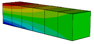
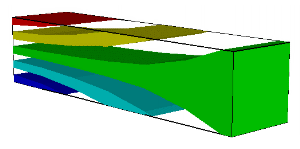
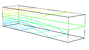
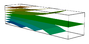
cantilever beam.

5 Application examples

In this section the results of two 3D finite element models illustrate the capabilities of the present volume contouring algorithm.

The first example is a simple cantiveler beam with a row of six brick (hexahedron) finite elements, as shown in Fig.9 . This figure shows an iso-strip contouring of longitudinal stresses due to a vertical load applied at the tip of the beam. The purpose of this simple example is to characterize the four types of contouring treated by the algorithm. Figures 10, 11, and 12 show iso-line, iso-volume, and iso-surface contourings for the same stress response.

In Fig. 11, every other contour level is displayed to clarify the iso-volume visualization of the response levels. Fig.11 illustrates that iso-volume contouring is trivially obtained as a combination of iso-strip contour polygons on the model boundary with iso-surface contour patches.

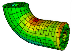
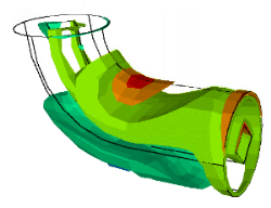
The second example is the analysis of a curved cylindrical tube with a square hole, as illustrated in Fig.13. This 3D finite element model contains 1280 brick elements and 1700 nodes. The adopted mesh and the iso-strip contouring of horizontal longitudinal stresses are shown in Fig.13. Fig.14 shows an iso-volume contouring of this model. Some contour levels are not displayed in this figure.

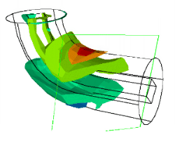
To demonstrate the capability of the proposed volume contouring algorithm in handling cells of arbitrary shape, the curved tube was sectioned at a plane as shown in Fig.15. As seen in this figure, the section plane divides some of the hexahedral elements into cells of several and random shapes. The resulting iso-volume contouring after the sectioning is shown in Fig.16.

Figure 13: Iso-strip contouring of
curved tube Figure 14: Iso-volume contoring of
curved tube Figure 15: Iso-strip contouring after
sectioning Figure 16: Iso-volume contouring after
sectioning

6 Conclusion

As a conclusion, it is interesting to compare the proposed method with others surface fitting algorithms. The marching cubes algorithm [6] is probably the most popular and efficient SF procedure. As its name implies, the procedure only considers hexahedral cells. The algorithm examines each cell and determines, from the arrangement of vertex values above or below a result threshold value, the topology of an iso-surface passing through this cell. The iso-surface is defined as patches of four or less triangles. These triangles are then passed to a rendering program that maps them to image space. There are exactly 256 ways that four or less triangles can be fit to a cell, and the number of cases can be reduced to 15 by reflection and rotation.

The marching cubes approach does not regard to neighbouring elements or the model as a whole, which can lead sometimes to connect the wrong set of three points while generating triangles, resulting in false positive or negative triangles in the iso-surface. One way to reduce ambiguous point connecting situations is to break up each cell into five, six or 24 tetrahedra. The marching tetrahedra algorithm [7] generates more triangles than the marching cubes, so more processing and memory are required.

The dividing cubes algorithm [8] takes advantage of the observation that the size of generate triangles, when rendered and projected, is often smaller than the size of a pixel. No intermediate surface primitives are used in the dividing cubes algorithm. Surface points are rendered into the image buffer using a standard algorithm such as the Z-buffer or the painter's algorithm. Rendering surface points instead of surface primitive saves a great deal of time.

Alternatively, the present volume contouring procedure allows iso-line, iso-strip, iso-surface, and iso-volume visualization of generic unstructured 3D meshes, such as finite element models. The algorithm can handle cells of any shape, even those that result from cutting off parts of the model through cutplanes. In fact, this was the main motivation for its development. This was done in a generic finite element post-processor [12], where any solid finite element could be considered and cutplanes can be specified.

A very important aspect of the proposed algorithm is that it integrates in the same methodology and data representation the four types of visualizations. As a consequence of this iso-volume contouring is trivially implemented as a combination of iso-strip and iso-surface patches of surfaces.

The proposed method assumes that an iso-surface of a specific value intercepts a generic cell smoothly (with no kinks) and only once. As mentioned previously, the first limitation is also present in the marching cubes and marching tetrahedra algorithms. The second limitation certainly restricts the classes of problems that can be visualized. However, as pointed out previously, it is consistent with the usual assumptions of the finite element method, which is the most popular method that uses unstructured meshes. One interesting consequence of this limitation is that the algorithm need not treat the ambiguity in point connection present in the marching cubes algorithm.

One problem with the present iso-surface generation is that it requires a local search for iso-line edge vertices along the faces of a cell. Although this search is efficient, certainly the surface fitting algorithm of the marching cubes procedure is more efficient than the present algorithm. The advantage here is that, while the marching cubes templates require cells of a fixed shape (a hexahedron), the present procedure can generate iso-surface patches for cells of any shape.

To give an idea of the computational efficiency of the present algorithm, the volumetric data of Fig.17 was processed by the marching cubes algorithm and the present algorithm. This figure shows an iso-surface of one value, after being cut, of a data set of 180x180x125 hexahedral cells, which generated 18870 iso-surface patches. On a Silicon Graphics Indigo 2 workstation, the elapsed time spent to generate these patches was 15.3 segs. for the marching cubes algorithm and 21.0 segs. for the proposed methods.

7 Acknowledgements

This work was developed at TeCGraf, Technology Group on Computer Graphics of PUC-Rio, which is supported by CENPES/Petrobras, CEPEL/Eletrobras, and other companies. The second author has a research grant from FAPERJ. This work was also partially supported by CNPq through GEOTEC project. The 3D finite element model used in section 5 was created using MG program of TeCGraf/Petrobras. For the model creation, special thanks are due to PUC-Rio Ph.D. students João Luiz Campos and Luiz Cristovão Gomes Coelho, and to Dr. Ivan Fábio Menezes. The authors are also greatful with M.Sc. student Flavio Szenberg for producing Fig.1 and Fig.2.

8 References

Publication Dates