Wave sequences for solid fuel adiabatic in-situ combustion in porous media

Wave sequences for solid fuel adiabatic in-situ combustion in porous media

A.J. de Souza^I; I.Y. Akkutlu^II; D. Marchesin^III

^IDepartamento de Matemática e Estatística, Universidade Federal de Campina Grande, Av. Aprigio Veloso, 882, 58109-970 Campina Grande, PB, Brazil. Email: [e-mail]

^IIDepartment of Civil and Environmental Engineering, University of Alberta, Edmonton, Canada, T6G 2W2. Email: [e-mail]

^IIIInstituto Nacional de Matemática Pura e Aplicada, Estrada Dona Castorina, 110, Jardim Botânico, 22460-320 Rio de Janeiro, RJ, Brazil. Email: [e-mail]

ABSTRACT

We study the Riemann problem with forward combustion due to injection of air into a porous medium containing solid fuel. We neglect air compressibility and heat loss to the rock formation. Given initial reservoir and injection conditions, we prove that there is a unique time asymptotic wave sequence for combustion with complete oxygen consumption. The sequence consists of a region of unburned air at injection temperature, a warming discontinuity, a hot region with unburned air, a combustion wave and a region with burned air and unburned fuel at the initial reservoir temperature. The waves have very different speeds, and therefore they cannot be detected in laboratory experiments that focus on the combustion wave. However, they should occur in field scale.

By introducing a cut-off in Arrhenius' law, the reaction rate vanishes at reservoir temperature, and two types of wave sequences are possible. One was already described. The other occurs for incomplete oxygen consumption. In this case, the wave sequence contains another wave, i.e., there is another region ahead of the combustion wave containing incompletely burned air at reservoir temperature, and a gas composition discontinuity that moves fast. However, instead of a unique solution for each Riemann data, there is a one parameter family of wave speeds and strengths. This multiplicity of solutions may to be due to the cut-off.

Mathematical subject classification: 80A25, 76S05.

Key words: coflow filtration combustion, porous media, Riemann solution.

1 Introduction

Air injection and in-situ combustion have long been considered as a potential technique for displacement and recovery of heavy oil reserves [7, 22]. Operational advantage of this thermal recovery technique is the abundance of injection gas independently of location. It utilizes heavy and immobile components of the crude oil as fuel producing in-place heat necessary for the recovery of upgraded crude oil.

Despite the advantages and a long history, only a small fraction of the total thermal recovery utilizes this technique. Some reasons are technical, such as the possibility of front extinction and the necessity of (re-)ignition for sustained propagation within in-situ combustion in the presence of external heat losses [1]. Thus mathematical analysis of this problem is important to predict these events.

A large number of studies on the structure of the combustion front have been reported since 1950s, see [1, 2, 3, 4, 5, 6, 8, 20, 21, 23, 26], for instance. These studies did not take into account other waves that occur in the combustion problem. As there is interaction between the combustion wave and other waves, this paper focuses on the solution of the Riemann problem with combustion taking into account all possible waves.

We assume that upstream processes during the in-situ combustion have already generated a stationary homogeneously distributed fuel. Burning of this fuel is the subject of the paper. A bimolecular reaction is assumed to take place between the injected oxygen and the solid fuel, hence the reaction region behaves as a source of heat as well as a sink for both of the reactants. We consider uniform flow, transport and reaction of injected air in porous medium of length l, with the reaction rate based on the Arrhenius' law. We neglect external heat losses. We develop simplified theoretical models for forward (co-flow) combustion under varying boundary conditions and obtain the wave sequences in the Riemann solution. The formulation of the problem is the same as in [4], while the nomenclature follows [1].

The paper is subdivided as follows. In Section 2 we present the mathematical model. Theory on systems of conservation laws suggests that, besides the combustion front, there could be rarefaction, shock or contact waves. In Section 3 we determine the characteristic speeds and prove that in this model there are neither rarefaction nor shock waves, only contact discontinuities. In fact, an examination of the Rankine-Hugoniot conditions shows that all noncombustion discontinuities are just the contact waves already found. In Section 4 we introduce the combustion front as a traveling wave of the evolution system derived in Section 2. In this section we also discuss the Rankine-Hugoniot jump conditions for the combustion wave. In Section 5 we prove that for the physical parameters considered in this paper, there are no resonances between waves, as opposed to the case analyzed by Aldushin et al. in [4]. As a consequence of the absence of resonances, we obtain two distinct temperature relationships for the combustion front, which we call the hot upstream and the hot downstream combustion cases. In Section 6 we determine the ranges of parameters in which these combustion waves may exist. In Section 7 we present our main results. For the hot upstream combustion we prove in Theorem 7.1 that the wave sequence of the Riemann solution is uniquely determined in case of complete consumption of oxygen. In Theorem 7.2 we prove that, for incomplete consumption of oxygen (using a modified version of the Arrhenius' law), there is another wave sequence as a solution. However, this solution is not unique, rather it is a one-parameter family of solutions. We also show that the hot downstream case does not occur in this model. In ^{Appendix A} we present tables with typical values of parameters, constants and nomenclature used through the paper.

2 Formulation of the problem

We assume that air is injected at the leftmost part of a porous rock cylinder containing solid fuel, so that all wave propagation is one dimensional. Balance equations are written for the total energy, the total gas mass, the oxygen mass and the fuel mass. For the latter, we define the fuel density per total volume r_f and introduce the extent of conversion depth, h = 1 – r_f/ is the initial fuel concentration), such that h = 0 corresponds to complete availability of fuel (denoted by superscript o) and h = 1 to the complete lack of fuel (the latter may occur because the fuel was never present or because it was completely consumed). The primary dependent variables are the temperature, , the oxygen concentration in terms of mass fraction, and the fuel conversion depth h. The gas density r_g is expressed by the ideal gas equation of state in terms of temperature and total gas pressure .

In formulating the conservation equations we make the following assumptions: the pore space and the solid matrix are in thermal equilibrium so that a one-temperature model is used for the energy balance; heat transfer by radiation, energy source terms due to pressure increase, and work from surface and body forces are all negligible; the ideal gas law is the equation of state for the gas phase; thermodynamic and transport properties, such as conductivity, diffusivity, heat capacity of the solid, heat of reaction, etc., all remain constant. We also neglect heat loss to the surrounding rock formation. We assume that gas heat capacity is negligible with respect to the rock heat capacity. The heat loss will be taken as zero as we study only the adiabatic case in this work. We assume that the pressure changes within any wave are negligible compared to the pressure drop across the system, so that in the ideal gas law and in other physical properties the pressure appears as a constant. Under these assumptions the dimensional form (indicated by the superscript tilde) of the energy balance, the oxygen mass balance, the gaseous phase mass balance and the combustion kineticsequations are:

where W is the reaction rate. The equations (2.1)-(2.3) were derived utilizing Darcy's law. The four equations (2.1)-(2.4) correspond to the three primary unknows , , h and the secondary unknow , which is the volumetric flow rate of the gas phase. In the above, c_i denotes the average specific heat capacity of species i (gas or solid) at constant pressure, r_i is the volumetric density of species i, is the effective thermal conductivity , is the heat released due to reaction (per unit mass of solid). Changes in the porosity f are considered to be negligible so that f is constant. D_M is an effective diffusion coefficient in the gas phase (D=D_M/f, where D is the molecular diffusion coefficient), while = M_o/M_f and _gp = _gpM_gp/ M_f are mass-weighted stoichiometric coefficients for oxygen and for combustion gaseous products, respectively. M_o, M_f and M_gp are the molecular weight of oxygen, fuel and gaseous products, respectively. The net gas mass production is determined from _g = _gp – , so that positive or negative sign for _g correspond to net gaseous phase mass production or consumption, respectively. We will assume _g > 0. For the rate of reaction, we use the second order law of mass action and the Arrhenius' Law:

with activation energy E and pre-exponential factor k_o.

We use the ideal gas equation of state

M_g = r_gR, where R is the universal gas constant, while M_g and r_g are the effective molecular weight and the effective density of the gas phase, respectively. We neglect the effect of changes of M_g due to the reaction by approximating M_g by a constant.

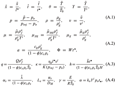
Non-dimensionalized combustion equations. We introduce dimensionless space and time variables. To bring out the internal structure of the combustion wave, we introduce convenient variables and parameters that are defined in ^{Appendix A}. We scale the length by l^*=a_s/vⁱ and the time using t^*=l^*/vⁱ, where vⁱ is the injection velocity and a_s the effective thermal diffusivity. We introduce the scaled temperature q = /₀, which means that the reservoir temperature corresponds to q₀ = 1; we also introduce the nondimensional gas density r, which is the gas density divided by the gas density at reservoir temperature. Thus the equations (2.1)-(2.4) are transformed into four dimensionless balance equations (2.6)-(2.9), while the dimensionless ideal gas law becomes Eq. (2.10):

where

The domain of the dependent variables is given by

From now on, we write ® t, ® x.

The values of the parameters a, q, f, L_e, µ, µ_g, a and g are given in Table 1 of ^{Appendix A}.

3 Non-combustion waves for the model in hyperbolic framework

In the absence of combustion, the source terms representing mass transfer or sensible heat generation containing the factor F vanish on the right hand sides of system (2.6)-(2.10). Of course F vanishes for Y º 0 or hº 1. We focus in the waves for large times and long distances for which the second derivative terms are negligible. Let us first consider smooth solutions, so we can expand the derivatives in the remaining terms in Eqs. (2.6-2.9), manipulate Eqs. (2.7), (2.8), use Eq. (2.10) to eliminate r, obtaining:

The characteristic speeds of system (3.1)-(3.4) in increasing order and the corresponding characteristic vectors are:

It is easy to see that all characteristic speeds are constant along the integral curves defined by the corresponding characteristic vector fields, which means that all of them are associated to contact discontinuities, hence they satisfy the Rankine-Hugoniot conditions for (3.1)-(3.4), [25]. The characteristic speed l^h corresponds to an immobile discontinuity along which only h varies, l^q corresponds to a thermal discontinuity along which q and v vary and l^Y corresponds to a gas composition discontinuity along which only Y varies.

4 The combustion wave

We proceed next with the study of combustion wave propagation. The combustion wave encounters unburned states ahead and leaves burned states behind it.

We look for combustion fronts as steady traveling waves of system (2.6)-(2.11) with propagation speed V > 0 by setting x = – V and t = . In these moving nondimensional coordinates, after using Eq. (2.10) to eliminate r, the equations (2.6)-(2.9) read, after writing ® x:

In the adiabatic case studied here, reaction at the back of the combustion zone ceases due to complete lack of fuel, i.e., h^b=1 at –¥. This is fuel-deficient combustion. (Thus, there can be no second combustion wave behind the first one.) Since gas is injected we have Y^b = 1. The temperature and the velocity behind the combustion need to be calculated. Thus the boundary conditions behind this combustion front are generically given by:

where the superscript b means burned.

Ahead of the combustion zone we consider that there is abundant fuel, i.e., h^u = 0 at +¥, under two distinct conditions surrounding the combustion front. The first condition is the complete oxygen consumption case where we set Y^u = 0 at +¥. The second condition is the temperature-controlled case where we set q^u = 1 at +¥, and Y^u have to be determined. The study of this second case is of special interest in petroleum applications, as it represents a situation where oxigen advances faster than the combustion wave, and the breakthrough of oxigen at the producing well causes safety hazards and other operational difficulties. These conditions can be summarized in (4.6) and (4.7), respectively:

where the superscript u means unburned.

Integrating equations (4.1)-(4.3) from x to +¥ once, taking into account that h^u = 0 at x = +¥ and re-ordering, we get:

Next, we substitute the value of v given by equation (4.10) into (4.8) and (4.9), and substitute the value of F given by Eq. (2.11) into (4.11) to obtain the reduced system:

We warn the reader that the temperature-dependent exponential on the right hand side of equation (4.14) will be modified when the temperature-controlled case given by the boundary condition (4.7) is studied.

The existence of solutions of system (4.12)-(4.14) for the boundary conditions (4.5) and (4.6), or (4.7), connecting the burned state U^b º (q^b, Y^b, h^b; v^b) at x ® –¥ to the unburned state U^u º (q^u, Y^u, h^u; v^u) and x ® +¥ is studied in a separate work, [9, 10]. Such solution represents the profile of a traveling wave connecting the burned state to the unburned state. For large times, this traveling wave is regarded as a thin combustion shock, [11, 15]. The Rankine-Hugoniot condition relating the burned and unburned states is studied in the next subsection.

4.1 The Rankine-Hugoniot equations for the combustion wave

For the boundary conditions given in (4.5) at –¥ and in (4.6), or (4.7), at +¥, taking into account that ¶q/¶x, ¶Y/¶x and ¶h/¶x tend to zero as x tends to ±¥, the R.H.S. of equations (4.12)-(4.13) become:

and Eq. (4.14) becomes a trivial identity. Taking x ® –¥ in Eq. (4.10) we obtain a separate equation for v^b:

The solutions of the Rankine-Hugoniot equations (4.15)-(4.17) together with the equation F = 0 determine all pairs of left and right states that are equilibria of system (4.12)-(4.14), i.e., that have the potential of representing burned and unburned states associated to a combustion wave.

4.2 Geometric analysis of the Rankine-Hugoniot equations

Since l^Y is the particle speed of gas it is convenient to introduce the scaled combustion wave speed V^u(V, v^u) º V/l^Y(U^u) given by:

Here the superscript u in V^u reminds the reader that V was scaled by v^u. Equations (4.15) and (4.16) give q^b and Y^u in terms of V, v^u and q^u, or in terms of V^u and q^u as follows:

For a fixed value of q^u, Eq. (4.19b) represents q^b in terms of V^u as a hyperbola drawn schematically in Fig. 4.1, constructed for parameter values given in ^{Appendix A}. The hyperbola has vertical and horizontal asymptotes respectively at:

The intersections of this hyperbola with the horizontal and vertical coordinate axes occur at:

Since am_g < q notice that Eqs. (4.21) and (4.22) lead to > q^u and < < 1, respectively.

Remark 4.1. The constants and = q^b() in Fig. 4.2 are related to Eq. (4.20b) and will be explained in the text. The constant q_M is defined by Eq. (5.1) and = V^u(q_M) is obtained from (4.27).

Now let us consider Eq. (4.20b) for a fixed value of q^u. This equation represents Y^u in terms of V^u as another hyperbola, which is drawn schematically in Fig. 4.2. This hyperbola has vertical asymptote V^u = 1 and horizontal asymptote at = f + q^u (µ + µ_g)/f, which has no physical meaning; see the horizontal dashed line in Fig. 4.2.

The intersections of this hyperbola with the horizontal and vertical coordinate axes occur at:

Knowing the value of we define the scaled temperature value:

Notice that = 1 / < 1.

Remark 4.2. For the quantities in Fig. 4.1 and 4.2, corresponding to the parameters in Table 1, the inequalities 0 < < < < < 1 hold.

We have expressed q^b and Y^u in terms of V^u. Now, let us also express q^b in terms of the scaled combustion speed:

here the superscript b in V^b reminds the reader that V was scaled by v^b.

Using Eq. (4.17) we obtain:

Alternatively, instead of obtaining an expression for q^b as a function of V^u and q^u as in (4.19b), Eq. (4.15) could be utilized to find V^u as function of q^b and q^u:

Similarly V^b can be written in terms of q^b:

Fig. 4.3 shows schematically V^b(q^b). The denominator in Eq. (4.28) is quadratic in q^b and vanishes at the two real roots and , with < 0 and > q^u. Thus the graph of Eq. (4.28) possesses vertical asymptotes given by q^b = and q^b = . The graph possesses also a horizontal asymptote given by V^b = 0.

We recall that we are interested in forward combustion, so we restrict our attention to the case V > 0. From Eqs. (4.18) and (4.25) it follows that V^u > 0 and V^b > 0. Thus, only the portions in the first quadrant of the graphs in Figs. 4.1, 4.2 and 4.3 are considered.

We conclude that the geometric analysis performed in this section yields the following restrictions relating burned and unburned states:

where V^u, , , , and V^b are defined by equations in (4.18), (4.21), (4.22), (4.23), (4.24) and (4.25), respectively.

5 Wave resonances

We can expect that changes of wave structure in the combustion Riemann problem occur whenever two wave speeds coincide, either in the burned or in the unburned regions. In this way we could have an interchange of the relative position of two waves. For the parameter values in Table 1 such changes are ruled out for physically interesting temperature range by the following theorem about absence of resonances:

Theorem 5.1. Let q_M be defined by

Then in the physical domain defined by Eq. (2.12):

(a) the non-combustion waves have distinct speeds;

(b) the combustion, the immobile and the gas composition waves have distinct speeds;

(c) consider a combustion wave following a thermal wave, i.e., V < l^q(U^u). In the limit as they tend to have equal speed, the temperature at the left of the superposed waves is q^b = q_M.

(d) consider a thermal wave following a combustion wave, i.e., l^q(U^b) < V. In the limit as they tend to have equal speed, the temperature at the right of the superposed waves is q^u = q_M.

Proof.

(a) From equations (3.5)-(3.7) we obtain explicitly that

which means that there are no speed equalities among non-combustion waves.

(b) Since we are considering forward combustion there is no resonance between the combustion and the immobile wave.

From Eqs. (4.29) and (4.31), we have that 0 < V^u < 1 and 0 < V^b < 1, respectively. Since V^u = V/l^Y(U^u) and V^b = V/l^Y(U^b), it follows respectively that

(c) From Eqs. (3.6), (4.18) and (4.27), the combustion wave following a thermal wave tend to have the same speed if, and only if, V^u = af/(q^u + af), or

(d) The proof is analogous to that of (c), using Eqs. (4.25), (4.28) instead of Eqs. (4.18), (4.27). This conclude the proof of Theorem 5.1.

Direct calculations with the value of the parameters in Table 1 yield q_M» 24.21264641. This corresponds to an extremely large temperature value above 6000 K that is beyond physical interest in our case; even at temperatures lower than 6000 K we may expect that heat losses to the surrounding reservoir cannot be neglected. This value q_M defines a maximum temperature value, below which there are no speed coincidences. Thus we focus our attention to the temperature range 0 < q q_M.

So one conclusion of this section is that for physical values of temperature there are no resonances between waves in this model.

Remark 5.2. The case where the thermal wave speed coincides with the combustion wave speed yields high temperatures and therefore maximal combustion efficiency. It is called superadiabatic combustion, which is desirable in other practical applications. The structure of such a combustion wave was analyzed in [4].

Since V^u and V^b are both positive, by analyzing the first denominator in Eq. (5.4) one can see that the sign of (q^b – q^u) determines if V < l^q or V > l^q. Thus, our final conclusion in this section is that the following two temperature relationships for the combustion front are possible:

(A) Hot upstream (left)

(B) Hot downstream (right)

6 The admissible Rankine-Hugoniot locus for the combustion wave

Cases (A) and (B) in (5.5) and (5.6) yield distinct possibilities for the rangesof q^b, V^b, V^u and Y^u corresponding to distinct portions of the branches in Figs. 4.1, 4.2 and 4.3. Such ranges are called the admissible states for combustion waves. In the next two subsections we will obtain the admissible ranges, which are fully characterized by the value of V^u: the first one is < V^u < and the second one is 0 < V^u < .

6.1 Hot upstream

Since q^b > q^u (see Fig. 4.1) it follows that V^u > . As 0 < Y^b < 1 (see Fig. 4.2) it follows that V^u < .

Let us define

represented in Fig. 4.1 and obtained from Eq. (4.27), where q_M is the maximum value for the nondimensionalized temperature q defined in (5.1). Let us also define

represented in Fig. 4.3, where the expression V^b is defined in Eq. (4.28). Finally, let in Fig. 4.2 be defined as

By comparing the graphs in Figs. 4.1, 4.2 and 4.3, and taking into account the inequalities obtained through the previous sections we arrive at the following Lemma, which characterizes the admissible Hugoniot locus for hot upstream combustion waves:

Lemma 6.1. Let q^u be a fixed value of the scaled temperature in the range 0 < q^u < q_M. Then the inequalities

hold if, and only if all of the following inequalities hold:

We notice that condition (6.5) implies that q^b > q^u (see Figs. 4.1 and 4.3).

6.2 Hot downstream

Since 0 < q^b < q^u we see that 0 < V^u < , where was defined in (4.22). See Fig. 4.1. Let in Fig. 4.2 be defined as

where the function Y^u is defined by Eq. (4.20b).

As 0 < V^u < and 0 < q^b < q^u it follows that < Y^u < 1 and 0 < V^b < 1. See Figs. 4.2 and 4.3, respectively.

As in the previous case, by comparing the graphs in Figs. 4.1, 4.2 and 4.3, and taking into account the inequalities obtained throughout the previous sections we arrive at the following Lemma, which characterizes the admissible Hugoniot locus for hot downstream combustion waves:

Lemma 6.2. Let q^u be a fixed value of the scaled temperature in the range 0 < q^u < q_M. Then the inequalities

hold if, and only if all of the following inequalities hold:

7 Wave sequences in the Riemann solutions

We have completed in Section 5 the proof that there is no wave speed coincidence in our combustion problem for temperatures of physical interest. We have also determined in Section 6 the admissible ranges of the left and right states of the combustion wave along the Hugoniot locus for the hot upstream and the hot downstream combustion cases given in (6.4)-(6.7) and (6.9)-(6.12), respectively. We will show in Section 7.2 that the hot downstream combustion case is unacceptable for this model. In the hot upstream combustion case we will describe the wave sequence in the Riemann solution under the conditions (4.6) and (4.7) surrounding the combustion front, where the waves satisfy an extension of Lax speed inequalities.

7.1 Hot upstream combustion case

In the hot upstream combustion case the thermal wave precedes the combustion wave (l^q(U^b) < V), there is no temperature change ahead the combustion wave, which means that q^u = 1 (reservoir temperature) and q^b > q^u = 1. Thus, generically the wave sequence in the Riemann solution consists of a (perhaps trivial) immobile fuel shock, a thermal shock with speed l^q, a combustion front with speed V and a gas composition wave with speed l^Y. We denote this sequence of waves by means of the following convention:

The state Uⁱ = (qⁱ, 1, 0, vⁱ) denotes the injection conditions, U¹ = (qⁱ, 1, 1, vⁱ) denotes an intermediate state in the burned region, while U^b = (q^b, 1, 1, v^b) and U^u = (1, Y^u, 0, v^u) are the burned and the unburned states surrounding the combustion front and U⁰ = (1, 0, 0, v⁰) denotes the reservoir conditions at production. The values of qⁱ and vⁱ are given as boundary conditions, the values of q^u and Y^u are given by condition (4.6) or (4.7), but the speeds l^q, V, l^Y and the values of q^b, v^b, v^u and v⁰ have to be determined.

7.1.1 The hot upstream combustion in the oxygen deficient case

As discussed above, we have that q^u = 1 and according to the condition (4.6), which characterizes the oxygen deficient case, Y^u = 0. We have the following theorem, which provides formulae for all the states as well as speeds for combustion and noncombustion waves in the wave sequence (7.1) for the Riemann solution in this case:

Theorem 7.1. Assume that in the wave sequence for the Riemann solution of (2.6)-(2.11) there is a hot upstream combustion wave with left and right states satisfying (4.5)-(4.6) and q^b > q^u = 1. Given the injection conditions Uⁱ = (qⁱ, 1, 0, vⁱ), with qⁱ > 0 and vⁱ > 0, then the constant states and the speeds of all waves in the wave sequence (7.1) are uniquely determined.

Proof. Inspecting Fig. 7.1 we see that the speeds and the intermediate states in the wave sequence (7.1) are determined as follows.

Substituting Y^u = 0 in Eq. (4.20b) it follows that V^u = , where is given in (4.23) with q^u = 1 (see Figs. 4.1 and 4.2). From Eq. (3.6) and Eq. (4.19b) with q^u = 1 and V^u = , it follows that:

Taking into account that the thermal wave is a contact discontinuity and Eq. (4.28) with q^u = 1 it follows that:

From Eq. (4.25) we obtain the combustion speed V; then we obtain v^u from Eq. (4.18):

Since Y^u = 0, the strength of the gas composition wave is zero, which explains why this wave is discarded in the wave sequence (7.1) as represented in Fig 7.1. Thus the proof of Theorem 7.1 is complete.

7.1.2 The hot upstream combustion in the temperature-controlled case

According to condition (4.7) we have q^u = 1, but Y^u have to be obtained.

First of all we notice that the condition (4.7) cannot be analyzed as (4.6) sincethe unburned state U^u is not an equilibrium of system (4.12)-(4.14), because F does not vanish. However the exponential factor in (2.5) is extremely small at prevailing temperatures, so we use the following modified version of the Arrhenius' law, [27]:

where E^b = E(^b – ₀)/ ^b.

This modification on the denominator in the exponential factor ensures that the reaction rate is equal to zero below the reservoir temperature

₀, which is a good approximation of the original formula in the Arrhenius' law. The value of E^b is chosen so that at the burned state above reservoir temperature the exponent assumes the same values as in the original Arrhenius' formula. Thus in the scaled temperature variable the function F in (2.11) is replaced by the approximation

F =

Y (1 – h) , for q > 1 and F = 0 for q < 1 .

With the above modified version of Arrhenius' law, the unburned state U^u becomes an equilibrium of system (4.12)-(4.14) and the existence of traveling wave solutions can be obtained, [9].

Now we notice that since q^u = 1 the range for V^u in Eq. (6.4) can be restricted further to

is obtained from Eq. (4.23) with q^u = 1. Consequently we get

where and are obtained from Eqs. (4.19a) and (4.28), respectively.

We can prove the following theorem in this case:

Theorem 7.2. Assume that in the wave sequence for the Riemann solution of (2.6)-(2.11) there is a hot upstream combustion wave governed by version (7.2) of Arrhenius' law with left and right states satisfying conditions (4.5) and (4.7), and q^b > q^u = 1. Given the injection conditions Uⁱ = (qⁱ, 1, 0, vⁱ), with qⁱ > 0, vⁱ > 0 and any positive value of the scaled combustion wave speed V^u in the interval [, ] given in (7.3), then all the constant states and speeds of all waves in the wave sequence (7.1) is uniquely determined.

Proof. Inspecting Fig. 7.2, we see that if the injection rate vⁱ, the temperature qⁱ and the value of V^u are given, then the speeds l^q, V and l^Y as well as the values of q^b, v^b, Y^u, v^u and v⁰ are determined as follows.

From Eq. (3.6) and Eq. (4.19) with q^u = 1, we have:

Taking into account that the thermal wave is a contact discontinuity and Eq. (4.28) with q^u = 1 it follows that:

From Eq. (4.25) we obtain the combustion speed V; then we obtain v^u from Eq. (4.18). From Eq. (4.20b) with q^u = 1, we obtain Y^u and from Eq. (3.7) with v = v^u, we obtain the value of l^Y:

Finally, since the gas composition wave is a contact discontinuity it follows that v⁰ = v^u , which provides a consistent solution of the system of conservation laws in the hyperbolic framework under the conditions (4.5)-(4.7) for left and right states to the combustion wave. This completes the proof of Theorem 7.2.

Remark 7.3. We notice that, due to the fact that the combustion and the thermal waves are very slow, it takes a long time for these waves to separate from each other, while the gas composition wave (the extremely fast wave) separates from the others immediately. This should explain why such phenomena have not been detected in laboratory experiments, where transient rather than asymptotic behavior is detected.

Remark 7.4. As we have seen in Theorem 7.2, in this case the injection conditions together with the initial data are not sufficient to determine the Riemann solution uniquely, but they determine a family of Riemann solutions depending on the parameter V^u. This strange multiplicity of solutions for the Riemann problem may to be related to the modification of the exponential factor (7.2) in Arrhenius' law.

Remark 7.5. There are two types of Riemann solutions for any given data if we use the modified version of Arrhenius' law: the regular solution for oxygen-controlled combustion and the one-parameter family of solutions for temperature-controlled combustion.

7.2 Hot downstream combustion

Recall that in the hot downstream combustion case we have to restrict the parameters to the ranges defined by Eqs. (6.9)-(6.12). Since 0 < < Y^u < 1 the complete oxygen consumption case defined by Eq. (4.6) is impossible.

Remark 7.6. We conclude that this model does not support case (b) of Aldushin et al. [4] that they call the reaction trailing structure.

In the temperature-controlled case defined by (4.7), under the standard Arrhenius' law (2.5) the state ahead the combustion front is not an equilibrium of the system of ordinary differential equations (4.12)-(4.14). This fact can be verified by a procedure analogous to that employed in Subsection 7.1.2. Thus the traveling wave technique is not applicable. On the other hand, if we use version (7.2) of Arrhenius' law we must set q^u = 1 and therefore we should have q^b < 1 in the downstream combustion case. Thus dh/dx is alway zero, i.e., there is no fuel consumption near the unburned state U^b and there is no connection between the equilibria U^b and U^u.

8 Discussion

We have seen that the original formulation of the Arrhenius' law allows us to describe mathematically the combustion front as a traveling wave for hot upstream combustion with complete oxygen consumption ahead the combustion front. In this situation we have proved that the wave sequence in the Riemann solution is uniquely determined by the injection conditions together with the initial data.

For incomplete oxygen consumption, or temperature-controlled case, theoriginal formulation is inappropriate to characterize the combustion front as a traveling wave, since the unburned state is not an equilibrium point of theassociated ordinary differential equation system. In such case, in order to apply the traveling wave theory a change of the Arrhenius formula can be used so that the unburned state becomes an equilibrium. As a consequence of this change of the Arrhenius' law, we lose uniqueness of Riemann solutions. Although the wave sequence is similar to that for the complete oxygen consumption case, the intermediate constant states and the wave speeds form a family depending on one parameter.

It is hard to establish the existence of traveling waves, which is assumed inthis work. Very often we are led to non hyperbolic equilibria of the associated system of ordinary differential equations in high dimensional spaces. Even in cases where the analysis can be done by the invariant manifold theory, weestablish the existence, but without explicit formulas, which would be very useful [13, 17, 19]. Of course, an alternative approach to be used together the invariant manifold theory is the singular perturbation theory, also called "matched asymptotic expansion", in which explicit approximations of the traveling wave solution can be obtained, [9, 12 14, 16, 24]. This is the subject of a separate work, [10].

Acknowledgments. We thank José Koiller, Grigori Chapiro, Yannis Yortsos and the Referees for their valuable contributions to this paper.

This work was supported in part by CNPq under Grants 300204/83-3, 523258/ 95-0, 306609/2004-5, and CNPq/PADCT 620017/2004-0; FINEP under CTPETRO Grant 21.01.0248.00 and CNPq/IM-AGIMB.

Received: 06/X/04. Accepted: 08/VIII/05.

#617/04.

In Eqs. (2.6)-(2.12), we introduced the following variables and parameters

where p_o corresponds to the initial gas pressure and is typically much larger than the pressure drop across the system.

• [1] I.Y. Akkutlu, Dynamics of Combustion Fronts in Porous Media, Ph. D. Thesis, Department of Chemical Engineering, University of Southern California, 2002.
• [2] I.Y. Akkutlu and Y.C. Yortsos, The Effect of Heterogeneity on In-situ Combustion: The Propagation of Combustion Fronts in Layered Porous Media, J. Pet. Tech., 54(6) (2002), 56-56.
• [3] I.Y. Akkutlu and Y.C. Yortsos, The Dynamics of In-situ Combustion Fronts in Porous Media, J. of Combustion and Flame, 134 (2003), 229-247.
• [4] A.P. Aldushin, I.E. Rumanov and B.J. Matkowsky, Maximal Energy Accumulation in a Superadiabatic Filtration Combustion Wave, Combustion and Flame, 118 (1999), 76-90.
• [5] H.R. Baily and B.K. Larkin, Conduction-convection in Underground Combustion, Petroleum Trans. AIME, 217 (1960), 321-331.
• [6] A.L. Benham and F.H. Poettmann, The Thermal Recovery Process - An Analysis of Laboratory Combustion Data, Petroleum Trans. AIME 213 (1958), 406-408.
• [7] T.C. Boberg, Thermal Methods of Oil Recovery, An Exxon Monograph Series (1988).
• [8] I.S. Bousaid and H.J. Ramey Jr., Oxidation of Crude Oil in Porous Media, Soc. Pet. Eng. J., 8(2) (1968),137-148.
• [9] G. Chapiro, Singular Perturbation Applied to Combustion Waves in Porous Media (in Portuguese), MSc Thesis, IMPA (2005).
• [10] G. Chapiro, D. Marchesin, A.J. Souza and A.A. Mailybaev, Singular perturbation of combustion waves in porous media, In preparation (2005).
• [11] R. Courant and K. Friedricks, Supersonic Flow and Shock Waves, John Wiley & Sons, New York, NY (1948).
• [12] F. Dkhil, Travelling Wave Solutions in a Model for Filtration Combustion, Nonlinear Analysis, 58 (2004), 395-415.
• [13] N. Fenichel, Persistence and Smoothness of Invariant Manifolds for Flows, Indiana Univ. Math., 21 (1971), 193-226.
• [14] N. Fenichel, Geometric Singular Perturbation Theory for Ordinary Differential Equations, J. Diff. Eq., 31 (1979), 53-98.
• [15] I. Gelfand, Some Problems in the Theory of Quasi-linear Equations, Uspekhi Mat. Nauk, 14 (1959), 87-158.
• [16] P.V. Gordon, An Upper Bound of the Bulk Burning Rate in Porous Media Combustion, Nonlinearity, 16 (2003), 2075-2082.
• [17] M. Hirsch, C. Pugh and M. Shub, Invariant Manifolds, Springer-Verlag, Lectures Notes in Math., 583 (1976).
• [18] J.C. Mota, D. Marchesin and W.B. Dantas, Combustion Fronts in Porous Media, SIAM Journal on Applied Mathematics, 62(6) (2002), 2175-2198.
• [19] J.C. Mota, A.J. Souza, R.A. Garcia and P.W. Teixeira, Oxidation Fronts in a Simplified Model for Two-Phase Flow in Porous Media, Matemática Contemporânea, 22 (2002), 67-82.
• [20] M. Kumar and A.M. Garon, An Experimental Investigation of the Fireflooding Combustion Zone, Soc. Pet. Eng. Res. Eng., 6(1) (1991), 55-61.
• [21] W.L. Martin, J.D. Alexander and J.N. Dew, Process Variable of In-situ Combustion, Petroleum Trans., 213 (1958), 28-35.
• [22] M. Prats, Thermal Recovery, SPE Monograph Series SPE of AIME (1982).
• [23] W.L. Penberthy and H.J. Ramey Jr., Design and Operation of Laboratory Combustion Tubes, Soc. Pet. Eng. J., 6(2) (1966), 183-198.
• [24] D.A. Schult, A. Bayliss and B.J. Matkowsky, Traveling Waves in Natural Counterflow Filtration Combustion and Their Stability, SIAM J. Appl. Math, 58(3) (1998), 806-852.
• [25] J. Smoller, Shock Waves and Reaction-Diffusion Equations, Springer-Verlag, Second Edition (1994).
• [26] L.A. Wilson, R.A. Reed, D.W. Reed and R.R. Clay, Some Effects of Pressure in Forward and Reverse Combustion, Soc. Pet. Eng. J., 3(2) (1963), 127-135.
• [27] Y.B. Zeldovich, G.I. Baremblatt, V.B. Librovich and G.M. Makhviladze, Mathematical Theory of Combustion and Explosion, Plenum (1985).

Appendix A.  Typical values, nomenclature and constants

Publication Dates

• Publication in this collection
  27 Sept 2006
• Date of issue
  2006

History

• Accepted
  08 Aug 2005
• Received
  06 Oct 2004