Abstract
In this article, third- and fourth-order accurate explicit time integration methods are developed for effective analyses of various linear and nonlinear dynamic problems stated by second-order ordinary differential equations in time. Two sets of the new methods are developed by employing the collocation approach in the time domain. To remedy some shortcomings of using the explicit Runge-Kutta methods for second-order ordinary differential equations in time, the new methods are designed to introduce small period and damping errors in the important low-frequency range. For linear cases, the explicitness of the new methods is not affected by the presence of non-diagonal damping matrix. For nonlinear cases, the new methods can handle velocity dependent problems explicitly without decreasing order of accuracy. The new methods do not have any undetermined algorithmic parameters. Improved numerical solutions are obtained when they are applied to various linear and nonlinear problems.
Keywords:
Linear and nonlinear dynamics; explicit time integration method; higher-order method
1 Introduction
Step-by-step direct time integrations are dominantly used for transient analyses of linear and nonlinear dynamic problems described by second-order ordinary differential equations in time. As more sophisticated spatial finite element models [1[1] J. N. Reddy. An Introduction to the Finite Element Method. McGraw-Hill New York, 3rd edition, 2006.
[2] O. C. Zienkiewicz and R. L. Taylor. The Finite Element Method for Solid and Structural Mechanics. Butterworth-Heinemann, 2005.
[3] D. Schillinger, J. A. Evans, F. Frischmann, R. R. Hiemstra, M. Hsu, and T. J. R. Hughes. A collocated c0 finite element method: Reduced quadrature perspective, cost comparison with standard finite elements, and explicit structural dynamics. International Journal for Numerical Methods in Engineering, 102(3-4):576-631, 2015.-4[4] W. Kim and J. N. Reddy. Novel mixed finite element models for nonlinear analysis of plates. Latin American Journal of Solids and Structures, 7(2):201-226, 2010.] are developed constantly, demands for more accurate time integration methods are also increasing to take full advantage of improved spatial models in transient analyses. Recently, numerous implicit [5[5] W. Kim and S. Y. Choi. An improved implicit time integration algorithm: The generalized composite time integration algorithm. Computers and Structures, 196:341-354, 2018.
[6] W. Kim and J. N. Reddy. An improved time integration algorithm: A collocation time finite element approach. International Journal of Structural Stability and Dynamics, 17(02):1750024, 2017.
[7] W. Kim and J. N. Reddy. A new family of higher-order time integration algorithms for the analysis of structural dynamics. Journal of Applied Mechanics, 84(7):071008, 2017.
[8] W. Kim and J. N. Reddy. Effective higher-order time integration algorithms for the analysis of linear structural dynamics. Journal of Applied Mechanics, 84(7):071009, 2017.-9[9] W. Kim, S. Park, and J. N. Reddy. A cross weighted-residual time integration scheme for structural dynamics. International Journal of Structural Stability and Dynamics, 14(06):1450023, 2014.] and explicit [10[10] J. Chung and J. M. Lee. A new family of explicit time integration methods for linear and non-linear structural dynamics. International Journal for Numerical Methods in Engineering, 37(23):3961-3976, 1994.
[11] G. M. Hulbert and J. Chung. Explicit time integration algorithms for structural dynamics with optimal numerical dissipation. Computer Methods in Applied Mechanics and Engineering, 137(2):175-188, 1996.
[12] D. Soares. An explicit family of time marching procedures with adaptive dissipation control. International Journal for Numerical Methods in Engineering, 100(3):165-182, 2014.
[13] D. Soares. A novel family of explicit time marching techniques for structural dynamics and wave propagation models. Computer Methods in Applied Mechanics and Engineering, 311:838-855, 2016.
[14] W. Kim and J. H. Lee. An improved explicit time integration method for linear and nonlinear structural dynamics. Computers and Structures, 206:42-53, 2018.
[15] W. Kim. A simple explicit single step time integration algorithm for structural dynamics. International Journal for Numerical Methods in Engineering, pages 00-00, 2019.-16[16] W. Kim. An accurate two-stage explicit time integration scheme for structural dynamics and various dynamic problems. International Journal for Numerical Methods in Engineering, pages 00-00, 2019.] time integration methods have been introduced to effectively analyze challenging dynamic problems.
Direct time integration methods are often categorized into implicit and explicit methods. Usually, implicit methods are unconditionally stable for linear analyses, but they require factorization of non-diagonal system matrices. For large systems, factorizing non-diagonal system matrices requires huge computational efforts. On the other hand, explicit methods are conditionally stable, but matrix factorization can be avoided if the mass matrix is diagonal. Accordingly, computational costs per time step of explicit methods are much lower than implicit methods. Due to this reason, explicit methods are more frequently used in analyses of large systems, such as the wave propagation and impact problems, where sizes of optimal time steps are slightly smaller than critical time steps of explicit methods.
According to the past studies [10[10] J. Chung and J. M. Lee. A new family of explicit time integration methods for linear and non-linear structural dynamics. International Journal for Numerical Methods in Engineering, 37(23):3961-3976, 1994.,17[17] M. A. Dokainish and K. Subbaraj. A survey of direct time-integration methods in computational structural dynamics i. explicit methods. Computers and Structures, 32(6):1371-1386, 1989.], preferable attributes of explicit time integration methods can be summarized as (a) explicit methods should not require iterative solution finding procedures for velocity dependent nonlinear problems; (b) at least second-order accuracy should be ensured; (c) number of unspecified algorithmic parameters should be minimized; (d) amplification matrices obtained by applying methods to the single-degree-of-freedom problem should not present spurious eigenvalue, or it should be minimized; (e) explicit methods should not involve matrix factorization when the mass matrix is diagonal; (f) explicit methods should not involve differential or integral type calculus; (g) explicit methods should be applicable to nonlinear problems without any modifications.
The central difference (CD) method is one of the most widely used single-stage explicit time integration methods. The CD method is second-order accurate and non-dissipative. Due to its simplicity and good accuracy, the CD method is the standard explicit method of the well-known software packages [18[18] T. J. R. Hughes. The Finite Element Method: Linear Static and Dynamic Finite Element Analysis. Dover, 2012.,19[19] K. J. Bathe. Finite Element Procedures. Klaus-Jurgen Bathe, 2006.]. However, matrix factorization is required in the CD method if the damping matrix is not diagonal. The velocity can be treated explicitly to remedy this, but additional computation is required to retain second-order accuracy [15[15] W. Kim. A simple explicit single step time integration algorithm for structural dynamics. International Journal for Numerical Methods in Engineering, pages 00-00, 2019.]. The CD method cannot satisfy (a) and (b).
Chung and Lee developed a family of second-order accurate explicit method [10[10] J. Chung and J. M. Lee. A new family of explicit time integration methods for linear and non-linear structural dynamics. International Journal for Numerical Methods in Engineering, 37(23):3961-3976, 1994.] with dissipation control capability. The Chung and Lee (CL) method can maintain explicitness in the presence of the non-diagonal damping matrix. However, the amplification matrix of the CL method has a spurious eigenvalue that influences the quality of solutions when large time steps are used. Hulbert and Chung also developed a family of second-order accurate explicit method [11[11] G. M. Hulbert and J. Chung. Explicit time integration algorithms for structural dynamics with optimal numerical dissipation. Computer Methods in Applied Mechanics and Engineering, 137(2):175-188, 1996.]. However, the amplification matrix of the Hulbert and Chung (HC) method also has a spurious eigenvalue. The HC method can satisfy all the attributes except (d). The HC method can include a full range of dissipative cases, but the non-dissipative case becomes unconditionally unstable for any choices of time steps in the presence of the damping matrix.
Soares developed an explicit time integration method based on the weighted residual method [13[13] D. Soares. A novel family of explicit time marching techniques for structural dynamics and wave propagation models. Computer Methods in Applied Mechanics and Engineering, 311:838-855, 2016.]. The Soares method can be used for the analysis of wave propagation problems, but it becomes an only first-order accurate implicit method in the presence of non-diagonal damping matrix. In addition, it is not easy to use the Soares method for nonlinear analyses, because it has been developed by directly integrating the equations of linear structural dynamics in a weighted residual sense. The Soares method cannot satisfy (a), (b), (d), (e), (f) and (g).
Kim and Lee also proposed a family of second-order accurate explicit methods [14[14] W. Kim and J. H. Lee. An improved explicit time integration method for linear and nonlinear structural dynamics. Computers and Structures, 206:42-53, 2018.]. The Kim and Lee (KL) method can include a full range of dissipative cases and remain as a second-order explicit method in the presence of a non-diagonal damping matrix. The KL method is very effective, but (c) is not satisfied. Recently, a very accurate two-stage explicit method was introduced by Kim [16[16] W. Kim. An accurate two-stage explicit time integration scheme for structural dynamics and various dynamic problems. International Journal for Numerical Methods in Engineering, pages 00-00, 2019.] to more effectively tackle challenging nonlinear problems.
For more precise and reliable analyses of challenging dynamic problems [20[20] W. Kim and J. Lee. A comparative study of two families of higher-order accurate time integration algorithms. International Journal of Computational Mechanics, accepted.], higher-order accurate methods can be considered as a good option. Many of the standard time integration methods used in structural dynamics, such as the trapezoidal rule and the central difference method, are second-order accurate, and methods of third- or higher-order accuracy are often called higher-order methods [7[7] W. Kim and J. N. Reddy. A new family of higher-order time integration algorithms for the analysis of structural dynamics. Journal of Applied Mechanics, 84(7):071008, 2017.,21[21] Gregory M Hulbert. A unified set of single-step asymptotic annihilation algorithms for structural dynamics. Computer Methods in Applied Mechanics and Engineering, 113(1-2):1-9, 1994.
[22] T.C. Fung. Unconditionally stable higher-order accurate hermitian time finite elements. International journal for numerical methods in engineering, 39(20):3475-3495, 1996.
[23] T.C. Fung. Weighting parameters for unconditionally stable higher-order accurate time step integration algorithms. part 2second-order equations. International journal for numerical methods in engineering, 45(8):971-1006, 1999.-24[24] T.C Fung. Unconditionally stable higher-order accurate collocation time-step integration algorithms for first-order equations. Computer methods in applied mechanics and engineering, 190(13-14):1651-1662, 2000.]. Computational cost per time step of higher-order methods is higher than second-order methods because higher-order methods have more stages, while many of second-order methods use only one stage. However, more accurate predictions can be obtained with large time steps in higher-order methods, and they may become more efficient in getting the same prediction when compared with second-methods. In addition, some challenging nonlinear problems can only be effectively solved by using proper higher-order methods [7[7] W. Kim and J. N. Reddy. A new family of higher-order time integration algorithms for the analysis of structural dynamics. Journal of Applied Mechanics, 84(7):071008, 2017.,8[8] W. Kim and J. N. Reddy. Effective higher-order time integration algorithms for the analysis of linear structural dynamics. Journal of Applied Mechanics, 84(7):071009, 2017.].
One of the most broadly used explicit higher-order methods is the Runge-Kutta (RK) methods. The RK methods have been used in numerous engineering areas. Traditionally, the RK methods have been used to solve first-order ordinary differential equations numerically. Recently, on the other hand, the RK methods have also been used to obtain higher-order accurate transient solutions in structural problems [25[25] J. A. Evans, R. R. Hiemstra, T. J. R. Hughes, and A. Reali. Explicit higher-order accurate isogeometric collocation methods for structural dynamics. Computer Methods in Applied Mechanics and Engineering, 338:208-240, 2018.].
For second-order initial value problems, the RK methods can provide more accurate numerical solutions than second-order methods if considerably small time steps are used. For example, the convergence rate of the four-stage RK method is fourth-order, and numerical solutions of the four-stage RK method converge to the exact solution with the rate of where is the size of the time step. In second-order methods, on the other hand, their numerical solutions converge to the exact solution with the rate of as decreases. However, numerical solutions of the RK methods may become inaccurate by the excessive numerical damping if large time steps are used. For this reason, the RK methods were not recommended for the analysis of structural dynamics, while many second-order explicit methods gained popularity. Adeli, Gere, and Weaver stated that the CD method was more effective than the RK method based on their numerical results [26[26] H. Adeli, J. M. Gere, and W. Weaver. Algorithms for nonlinear structural dynamics. Journal of the Structural Division, 104(2):263-280, 1978.], and many researchers also agreed with that. In the numerical tests of Adeli et al., the fourth-order RK method introduced too excessive numerical damping in the important low-frequency range when large time steps were used.
In this work, simple and effective third- and fourth-order accurate explicit time integration methods are presented to remedy the shortcomings of the RK methods. For a fair comparison, the three-stage third-order accurate RK method and the four-stage fourth-order accurate RK method are considered. Higher-order accuracies of the new methods are achieved without increasing computational efforts when compared with the equivalent third- and fourth-order RK methods. In the development, the displacement vector is approximated over a time domain by using the known interpolation functions in time and the weighted sums of acceleration vectors. Then, the semi-discrete equations of structural dynamics are discretized in time by adopting the collocation method. After determining optimal collocation points in time, simple difference relations are obtained.
2 New explicit method
The governing equations of many dynamic problems can be expressed as
and the initial conditions are given by
where is the mass matrix, is the displacement vector, is the velocity vector, is the acceleration vector, is the initial displacement vector, is the initial velocity vector, and is the total force vector. Eq.(1) is suitable for the description of various linear and nonlinear dynamic problems. In linear structural dynamics, in Eq.(1) is frequently expressed as
where and are the damping and stiffness matrices, respectively, and is the external force vector. By substituting Eq.(2) into Eq.(1a) and rearranging the equation, the equation of linear structural dynamics is expressed as
Occasionally, Eq.(3) can also be obtained by spatially discretizing original governing partial differential equations in space and time. Then, Eq.(3) is also called the semi-discrete equation.
In this section, two sets of new higher-order explicit methods are developed to discretize Eqs.(1) and (3) in time. The single-degree-of-freedom case of the linear structural dynamics equation given in Eq.(3) is used in the procedures of the development.
2.1 New third-order accurate explicit method
For the development of the new third-order accurate explicit method, three sets of interpolation functions in time are used to approximate the displacement and velocity vectors over the time domain , where is the local time, and is the beginning of the -th time step or the end of the -th time step. In the new third-order method, the displacement and velocity vectors at are approximate as
where determines the time point that the first approximated variables are associated with, is computed explicitly by using Eq.(1a) at , s are the known linear functions, and is the weighting parameter of the acceleration vector in the first approximation of the displacement vector. s used in Eqs.(4) and (5) are given by
The displacement and velocity vectors at are approximate as
where determines the time point that the first approximated variables are associated with, is computed explicitly by using Eq.(1a) at , s are the known quadratic interpolation functions, and and are the weighting parameters of the acceleration vectors in the second approximation of the displacement vector. s used in Eqs.(7) and (8) are given by
Finally, the displacement and velocity vectors at are updated as
where is computed explicitly by using Eq.(1a) at , s are the known cubic interpolation functions, and , , and are the weighting parameters of the acceleration vectors in the third approximation of the displacement vector. s used in Eqs.(10) and (11) are given by
To achieve third-order accuracy, extended stability, and preferable spectral properties, permissible and are chosen as
By using the parameters given in Eq.(13) and rearranging the equations, the new third-order method are summarized as follow: To start the new third-order explicit method, compute the acceleration vector at as
where and are known properties from -th time step. By using Eq.(14), the displacement and velocity vectors at are approximated as
By using and given in Eqs.(15) and (16), the acceleration vector at is computed as
By using Eq.(17), the displacement and velocity vectors at are approximated as
By using and given in Eqs.(18) and (19), the acceleration vector at is computed as
Finally, the displacement and velocity vectors at are computed as
As shown in Eqs.(14)-(22), is the only matrix factorization required through out the entire procedure. This trait is commonly found in the existing explicit methods, and total computational effort of analyses can be reduced dramatically when is diagonal. Also, some recent numerical integration techniques [3[3] D. Schillinger, J. A. Evans, F. Frischmann, R. R. Hiemstra, M. Hsu, and T. J. R. Hughes. A collocated c0 finite element method: Reduced quadrature perspective, cost comparison with standard finite elements, and explicit structural dynamics. International Journal for Numerical Methods in Engineering, 102(3-4):576-631, 2015.] can produce diagonal mass matrix automatically if low order spatial elements are considered. After computing and , and are updated as and to advance another step, and procedures can be repeated from Eq.(14) to Eq.(22).
2.2 New fourth-order accurate explicit method
The new fourth-order method is developed by considering an additional stage. In the new fourth-order accurate method, the first and second approximations of the displacement and velocity vectors take the same forms as the approximations used in the third-order method given in Eqs.(4)-(8). The third approximations of the fourth-order method at take the forms of
where determines the time point that the third approximated variables are associated with, and is computed explicitly by using Eqs.(7)-(8) and Eq.(1a) at . The displacement and velocity vectors at are updated as
where is computed explicitly by using Eqs.(23)-(24) and Eq.(1a) at, s are the known quartic interpolation functions, and , , , and are the weighting parameters of the acceleration vectors in the fourth approximation of the displacement vector. s used in Eqs.(25) and (26) are given by
To achieve fourth-order accuracy, extended stability, and preferable spectral properties, permissible and are chosen as
With the parameters given in Eq.(28), the new fourth-order method is summarized as follows: To start the new fourth-order explicit method, compute the acceleration vector at as
where and are known properties from -th time step. By using Eq.(14), the displacement and velocity vectors at are approximated as
By using and given in Eqs.(30) and (31), the acceleration vector at is computed as
By using Eq.(32), the displacement and velocity vectors at are approximated as
By using and given in Eqs.(33) and (34), the acceleration vector at is computed as
The interim displacement and velocity vectors at are approximated as
By using and given in Eqs.(36) and (37), the acceleration vector at is computed as
Finally, the displacement and velocity vectors at are computed as
After computing and , and are updated as and to advance another step, and procedures can be repeated from Eq.(29) to Eq.(40).
3 Review of the Runge-Kutta methods
The RK Methods are frequently used to analyze various linear and nonlinear dynamic systems described by first-order differential equations. Traditionally, the RK Methods have been considered unsuitable for the analysis of dynamic problems stated by second-order differential equations due to excessive numerical damping. Recently, however, the RK Methods have also been employed to develop a more accurate numerical procedure which can be used for the analysis of structural dynamics [25[25] J. A. Evans, R. R. Hiemstra, T. J. R. Hughes, and A. Reali. Explicit higher-order accurate isogeometric collocation methods for structural dynamics. Computer Methods in Applied Mechanics and Engineering, 338:208-240, 2018.]. In this section, the third- and fourth-order Runge-Kutta methods are reviewed briefly.
3.1 Third-order Runge-Kutta Method
In the third-order RK method, is computed as
The displacement and velocity vectors at are approximated as
is computed as
The interim displacement and velocity vectors at are approximated as
is computed as
Finally, the displacement and velocity vectors at are computed as
As shown in Eqs.(41)-(49), computational structures of the new third-order method and the third-order RK method are very similar. It can also be observed that each method contains three major computations (i.e., ). Due to this reason, computational cost per a step of each method is almost identical.
3.2 Fourth-order Runge-Kutta Method
In the fourth-order RK method, is computed as
The displacement and velocity vectors at are approximated as
is computed as
The displacement and velocity vectors at are approximated as
is computed as
The interim displacement and velocity vectors at are approximated as
is computed as
Finally, the displacement and velocity vectors at are computed as
As shown in Eqs.(50)-(61), computational structures of the new fourth-order method and the fourth-order RK method are very similar. It can also be observed that each method contains four major computations (i.e., ). Due to this reason, computational cost per a step of each method is almost identical.
4 Analysis of the new methods
In this section, numerical characteristics of the new methods are analyzed. To investigate numerical characteristics of time integration methods, the linear single-degree-of-freedom problem [27[27] T. J. R. Hughes. The finite element method: linear static and dynamic finite element analysis. Courier Corporation, 2012.
[28] T. J. R. Hughes. Analysis of transient algorithms with particular reference to stability behavior. Computational methods for transient analysis(A 84-29160 12-64). Amsterdam, North-Holland, 1983, pages 67-155, 1983.-29[29] H. M. Hilber. Analysis and design of numerical integration methods in structural dynamics. PhD thesis, University of California Berkeley, 1976.] is frequently used. The linear single-degree-of-freedom problem is given as
with the initial conditions
where is the displacement, is the initial displacement, is the initial velocity, is the damping ratio, is the natural frequency, and is the external force. By setting , , , , and and applying Eqs.(14)-(22) to Eqs.(62)-(63), fully discrete relation of the new third-order method at is given by
where is the amplification matrix of the new third-order method, is the load operator matrix of the new third-order method, , , and . By applying Eqs.(29)-(40) to Eqs.(62)-(63), fully discrete relation of the new fourth-order method at is given by
where is the amplification matrix of the fourth-order method, is the load operator matrix of the fourth-order method, and .
4.1 Order of accuracy
To investigate the order of accuracy of the new methods for linear problems, the characteristic polynomial of the amplification matrices is used. For a time integration method, the characteristic polynomial of the amplification matrix is expressed as
where is the eigenvalue of , and and are the invariants of . By using and , the local truncation error [28[28] T. J. R. Hughes. Analysis of transient algorithms with particular reference to stability behavior. Computational methods for transient analysis(A 84-29160 12-64). Amsterdam, North-Holland, 1983, pages 67-155, 1983.,29[29] H. M. Hilber. Analysis and design of numerical integration methods in structural dynamics. PhD thesis, University of California Berkeley, 1976.] is defined as
where is the exact solution of Eq.(62). For the case of , the exact solution is given by
where is the damped natural frequency. Then a method is -th order accurate if
The new third-order method gives
According to Eq.(69), the new three-stage method is third-order accurate for the damped case (), and it becomes forth-order accurate for the undamped case (). Thus, the new third-order method is expected to give more accurate solutions for the undamped cases when compared with the equivalent third-order RK method. The new four-stage method gives
and it is fourth-order accurate for the damped and undamped cases according to Eq.(71).
4.2 Spectral radius and stability limit
The spectral radius is frequently used to investigate linear stability of time integration method. The spectral radius is defined as
where and are the eigenvalues of . A method is stable if is provided. The spectral radii of the methods are presented in Fig.1. For the undamped case, the critical time step of the new third-order method is , where is the natural period. Thus, the new third-order method is stable if is provided. The critical time step of the new fourth-order method is . The stability limit slightly decreases as increases from 0.0 to 1.0 in the new methods. However, similar phenomena have been observed in many well-accepted explicit methods [10[10] J. Chung and J. M. Lee. A new family of explicit time integration methods for linear and non-linear structural dynamics. International Journal for Numerical Methods in Engineering, 37(23):3961-3976, 1994.,11[11] G. M. Hulbert and J. Chung. Explicit time integration algorithms for structural dynamics with optimal numerical dissipation. Computer Methods in Applied Mechanics and Engineering, 137(2):175-188, 1996.,30[30] G. Noh and K. J. Bathe. An explicit time integration scheme for the analysis of wave propagations. Computers and structures, 129:178-193, 2013.].
4.3 Period and damping error
The order of accuracy is one of the most important measurements for accuracy. However, the period elongation and the damping ratio are more practical measurements, because they can directly describe important characteristics of time integration algorithms. The relative period error is defined as where, the exact period is , and the numerically obtained period is . The algorithmic damping ratio is defined as, where and . For more details, please see Ref.[28[28] T. J. R. Hughes. Analysis of transient algorithms with particular reference to stability behavior. Computational methods for transient analysis(A 84-29160 12-64). Amsterdam, North-Holland, 1983, pages 67-155, 1983.].
The new third- and fourth-order explicit methods have much smaller damping and period errors when compared with the third- and fourth-order RK methods as shown in Figs.2 and 3. Based on the results presented in Fig.2, it can be expected that the new methods will give very small period error in long-term analyses. This will be verified by using various numerical examples in the next section. Fig.3 is showing that the new explicit methods do not introduce excessive numerical (or algorithmic) damping into the important low-frequency range, while considerable numerical damping is introduced in the RK methods.
5 Numerical examples
In this section, six illustrative examples are considered to demonstrate improved performances of the new methods. To keep the simplicity of the numerical analysis, only dimensionless problems are considered. Among the examples, two-degree-of-freedom nonlinear spring-pendulum and double pendulum problems are used to verify the performance of the proposed method for multi-degree-of-freedom problems. It should also be noted that the precision of 16 significant digits is used for evaluations of variables in the computer code.
As shown in Table 1, the computation times of the four different higher-order explicit methods are almost identical when the number of degree-of-freedoms is less than hundred. As degree-of-freedoms increase, on the other hand, the computation times of the third-order methods become approximately 75% of the fourth-order methods. As expected, computational times of the new explicit methods and the RK methods are almost the same when the same numbers of stages are assumed.
Computation times (in seconds) taken to obtain nonlinear numerical solutions of 10,000-th time step for varying sizes of system (i.e., degree-of-freedoms).
5.1 Single-degree-of-freedom problem
Eqs.(62) and (63) are solved by using the new methods and the RK methods. For undamped cases, , , , , and are used. For damped cases, , , , , and are used. and are used for both cases. All properties are dimensionless. As shown in Figs.4- 7, the new third- and fourth-order methods are presenting more accurate solutions when compared with the RK methods. The third-order RK method gives very inaccurate predictions when is used as shown in Figs.4 and 6. The reference solution is obtained by using the exact solution.
5.2 Elastic hardening spring problems
The hardening elastic spring problem is considered. The motion of a hardening elastic spring [31[31] W. L. Wood and M. E. Oduor. Stability properties of some algorithms for the solution of nonlinear dynamic vibration equations. International Journal for Numerical Methods in Biomedical Engineering, 4(2):205-212, 1988.
[32] Y. M. Xie. An assessment of time integration schemes for non-linear dynamic equations. Journal of Sound and Vibration, 192(1):321-331, 1996.-33[33] J. Liu and X. Wang. An assessment of the differential quadrature time integration scheme for nonlinear dynamic equations. Journal of Sound and Vibration, 314(1):246-253, 2008.] is expressed as
where and . The elastic spring problem given in Eq.(73) is a conservative system. The total energy of the spring can be computed exactly by using the initial displacement and velocity. For the numerical test, , , , and are used [32[32] Y. M. Xie. An assessment of time integration schemes for non-linear dynamic equations. Journal of Sound and Vibration, 192(1):321-331, 1996.]. All properties are dimensionless. The nonlinear period of the problem is computed by using 10th-order implicit Kim and Reddy method [7[7] W. Kim and J. N. Reddy. A new family of higher-order time integration algorithms for the analysis of structural dynamics. Journal of Applied Mechanics, 84(7):071008, 2017.,20[20] W. Kim and J. Lee. A comparative study of two families of higher-order accurate time integration algorithms. International Journal of Computational Mechanics, accepted.] with time step . The nonlinear period of the problem is computed as . All methods used .
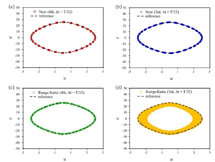
Phase portrait of the hardening spring problem , , , , and are used with to complete fifty cycles (i.e., until ). (a) New fourth-order method; (b) New third-order method; (c) Fourth-order RK method; (d) Third-order RK method.
Fifty cycles of displacement and velocity solutions are observed. Since this problem is conservative, the displacement-velocity portrait should form a closed cycle as depicted in Fig.8(a) and (b). The results presented in Fig.8 show that the phase portrait obtained by using the new methods is very accurate. Numerical solutions are forming thirty-two groups on the exact portrait when is used. However, the phase portraits obtained from the RK methods are scatted along the exact phase portrait as shown Fig.8(c) and (d).
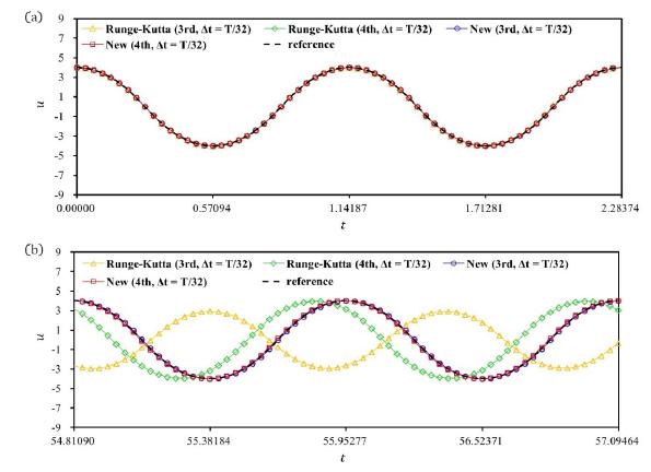
Displacement solution of the hardening spring problem , , , , and are used with. (a) short-term solutions (); (b) long-term solutions ().
The results presented in Fig.9 support the fact that the small period error of the new methods can improve the quality of solutions in long-term analyses.
5.3 Elastic softening spring problems
The softening equation [31[31] W. L. Wood and M. E. Oduor. Stability properties of some algorithms for the solution of nonlinear dynamic vibration equations. International Journal for Numerical Methods in Biomedical Engineering, 4(2):205-212, 1988.
[32] Y. M. Xie. An assessment of time integration schemes for non-linear dynamic equations. Journal of Sound and Vibration, 192(1):321-331, 1996.-33[33] J. Liu and X. Wang. An assessment of the differential quadrature time integration scheme for nonlinear dynamic equations. Journal of Sound and Vibration, 314(1):246-253, 2008.] is also solved by using the new methods. The motion of the softening elastic spring is expressed as
where . Here we use,, and [32[32] Y. M. Xie. An assessment of time integration schemes for non-linear dynamic equations. Journal of Sound and Vibration, 192(1):321-331, 1996.]. All properties are dimensionless. Fifty cycles of displacement and velocity solutions are observed. This problem is also conservative, and exact displacement-velocity portrait should form a closed cycle as depicted in Fig.10(a), (b) and (c). The results presented in Fig.10 show that the phase portrait obtained by using the new methods is accurately forming 32 groups on the exact portrait of the displacement-velocity when is used. The phase portrait obtained from the fourth-order RK method is less accurate than the new methods. On the other hand, the phase portrait obtained from the third-order RK method is approaching toward the origin. The third-order RK method exhibits the most inaccurate result as shown in Fig.10(d). As shown in Fig.10(d), the third-order RK method becomes excessively dissipative when a large time step is used.
The results presented in Fig.11 also support the fact that the small period and damping errors of the new methods can improve the quality of numerical solutions in long-term analyses.
Phase portrait of the hardening spring problem , ,, andare used with to complete fifty cycles (i.e., until ). (a) New fourth-order method; (b) New third-order method; (c) Fourth-order RK method; (d) Third-order RK method.
Displacement solution of the hardening spring problem , ,, andare used with. (a) short-term solutions (); (b) long-term solutions ().
5.4 Nonlinear single pendulum problem
Description of nonlinear single pendulum [5[5] W. Kim and S. Y. Choi. An improved implicit time integration algorithm: The generalized composite time integration algorithm. Computers and Structures, 196:341-354, 2018.]
The nonlinear oscillation of single pendulum described in Fig.12 is numerically solved. The motion of the single pendulum is described
with initial conditions
where is, is the angle between the rigid rod and the vertical line at time, is the gravitational constant, and is the length of the massless rigid rod. Dimensionless values and are used in the example.
This simple nonlinear pendulum problem is suitable for the test of time integration methods, because important information regarding motions of the pendulum (such as the period and the maximum angle) can be exactly computed by using the initial conditions given in Eqs.(76a) and (76b). For details, please see Refs.[5[5] W. Kim and S. Y. Choi. An improved implicit time integration algorithm: The generalized composite time integration algorithm. Computers and Structures, 196:341-354, 2018.], [34[34] T. C. Fung. Solving initial value problems by differential quadrature method-part 2: second and higher-order equations. International Journal for Numerical Methods in Engineering, 50(6):1429-1454, 2001.], and [35[35] T. C. Fung. On the equivalence of the time domain differential quadrature method and the dissipative runge-kutta collocation method. International Journal for Numerical Methods in Engineering, 53(2):409-431, 2002.].
For the test of the new methods, two sets of initial conditions are used. First, the initial conditions that have been used in Refs.[5[5] W. Kim and S. Y. Choi. An improved implicit time integration algorithm: The generalized composite time integration algorithm. Computers and Structures, 196:341-354, 2018.,7[7] W. Kim and J. N. Reddy. A new family of higher-order time integration algorithms for the analysis of structural dynamics. Journal of Applied Mechanics, 84(7):071008, 2017.,14[14] W. Kim and J. H. Lee. An improved explicit time integration method for linear and nonlinear structural dynamics. Computers and Structures, 206:42-53, 2018.] are also used in this study to synthesize a highly nonlinear case where the pendulum oscillates continuously between two peak points not making complete turns. Second, the initial conditions are chosen as and to synthesize a highly nonlinear case where pendulum makes complete turns about the point . These initial conditions can synthesize even more challenging problem than the case used in Ref.[14[14] W. Kim and J. H. Lee. An improved explicit time integration method for linear and nonlinear structural dynamics. Computers and Structures, 206:42-53, 2018.]. Mathematically computed period of the first set of the initial conditions is 33.72102056501721, and numerically computed period of the second set of the initial conditions is 33.7210. Interestingly, periods of the two cases are almost identical. is used for each set of initial conditions.
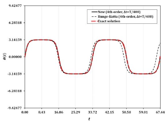
Angles of the oscillating nonlinear single pendulum problem described in Fig.12(a) for varying values of . The new third-order explicit method and the third-order Runge-Kutta method are used, and is selected as for both methods, where .
Angles of the oscillating nonlinear single pendulum problem described in Fig.12(a) for varying values of . The new fourth-order explicit method and the third-order Runge-Kutta method are used, and is selected as for both methods, where .
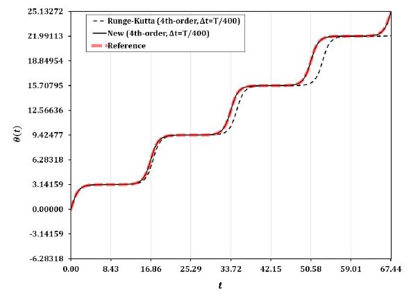
Angles of the rotating nonlinear single pendulum problem described in Fig.12(b) for varying values of . The new third-order explicit method and the third-order Runge-Kutta method are used, and is selected as for both methods, where .
Angles of the rotating nonlinear single pendulum problem described in Fig.12(b) for varying values of . The new fourth-order explicit method and the third-order Runge-Kutta method are used, and is selected as for both methods, where .
Comparison of relative error at . at is analytically computed as 3.13984732433779890888572.
For the first set of the initial conditions, the numerical solution of the new third-order method is almost superposing the exact solution (the dotted red line) as shown in Fig.13. However, the third-order RK method is presenting noticeable period error as shown in Fig.13. The numerical solutions of the new fourth-order methods are completely superposing the exact solution (the dotted red line) as shown in Fig.14. On the other hand, the fourth-order RK method is showing better results when compared with the third-order RK method, but the period error is still noticeable as shown in Fig.14.
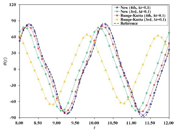
For the second set of the initial conditions, the numerical solution of the new third-order method is almost superposing the exact solution (the dotted red line) as shown in Fig.15. However, the third-order RK method is presenting huge period error and giving a completely incorrect prediction as shown in Fig.15. The result of the third-order RK method indicates that the pendulum is oscillating between the two peak points instead of making complete turns. The numerical solution of the new fourth-order method is completely superposing the exact solution (the dotted red line) as shown in Fig.16, while the fourth-order RK method is showing noticeable period error.
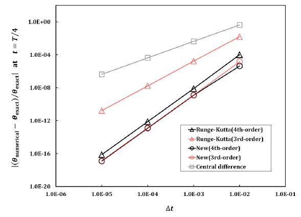
To investigate convergence rate of the nonlinear solutions obtained from various methods, the first set of the initial conditions is used. Errors at are computed and plotted as shown in Fig.17. The order of accuracies expected in the linear single-degree-of-freedom problem as given in Eqs.(70) and (71) are also achieved in this nonlinear problem.
5.5 Spring-pendulum problem
The two-degree-of-freedom spring-pendulum problem [10[10] J. Chung and J. M. Lee. A new family of explicit time integration methods for linear and non-linear structural dynamics. International Journal for Numerical Methods in Engineering, 37(23):3961-3976, 1994.] is used for the test of the new methods. The configuration of the two-degree-of-freedom spring-pendulum problem is described in Fig.18. The governing equations are given by
and the initial conditions are
where and are the displacements in the radial and circumferential directions, respectively, is the mass of the pendulum, is the gravitational constant, is the length of the undeformed spring, and is the spring constant. In this numerical test, , , , , , , and are used. All properties are dimensionless.
Description of spring pendulum [5[5] W. Kim and S. Y. Choi. An improved implicit time integration algorithm: The generalized composite time integration algorithm. Computers and Structures, 196:341-354, 2018.].
Comparison of relative error at . is computed by using the 10th-order accurate method of Kim and Reddy [7[7] W. Kim and J. N. Reddy. A new family of higher-order time integration algorithms for the analysis of structural dynamics. Journal of Applied Mechanics, 84(7):071008, 2017.,20[20] W. Kim and J. Lee. A comparative study of two families of higher-order accurate time integration algorithms. International Journal of Computational Mechanics, accepted.].
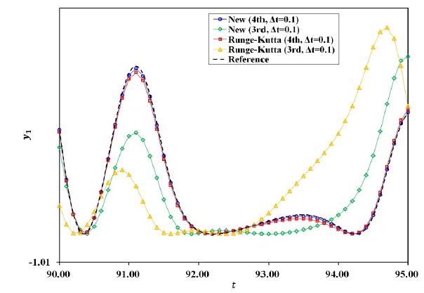
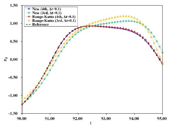
In this particular problem, the new fourth-order method is presenting accurate solutions while the new third-order method and the third- and fourth order RK methods are not as presented in Figs.19-20. Interestingly, the convergence rate of the new third-order explicit method for the spring-pendulum is third-order as shown in Fig.21. This is due to the velocity dependent nonlinearity included in the governing equations. The results presented in Fig.21 are in good agreement with the order of accuracy computed by using the linear single-degree-of-freedom problem given in Eqs.(70) and (71).
5.6 Double pendulum problem
A double pendulum problem described in Fig.22 is solve to test the new methods. This double pendulum problem can also be used to investigate chaos dynamics [36[36] S. Maiti, J. Roy, A. K. Mallik, and J. K. Bhattacharjee. Nonlinear dynamics of a rotating double pendulum. Physics Letters A, 380(3):408-412, 2016.].
The governing equations of the double pendulum [37[37] T. Stachowiak and T. Okada. A numerical analysis of chaos in the double pendulum. Chaos, Solitons & Fractals, 29(2):417-422, 2006.] is given by
where and are angle of the first and second pendulums, respectively, and are masses of the first and second pendulums, respectively, and are weightless rigid rods connected to pendulums as shown in Fig.22, and and are the initial angles. By using and , positions of the pendulum are computed as follows:
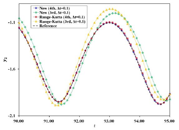
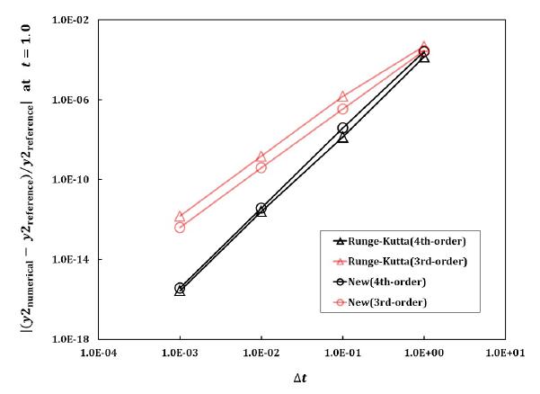
Dimensionless properties , , , , and are used, and the initial conditions are chosen as . All properties are dimensionless. In this particular problem, the new fourth-order method and the fourth-order RK method are presenting accurate solutions while the new third-order method and the third-order RK method are not as presented in Figs.23- 26. The new fourth-order method is presenting slightly more accurate result when compared with the fourth-order RK method. The convergence rates of the new explicit methods for the double-pendulum problem are presented in Fig.27.
Comparison of relative error at . is computed by using the 10th-order accurate method of Kim and Reddy [7[7] W. Kim and J. N. Reddy. A new family of higher-order time integration algorithms for the analysis of structural dynamics. Journal of Applied Mechanics, 84(7):071008, 2017.,20[20] W. Kim and J. Lee. A comparative study of two families of higher-order accurate time integration algorithms. International Journal of Computational Mechanics, accepted.].
6 Concluding remarks
The new third- and fourth-order explicit methods presented in this paper could provide accurate numerical solutions when applied to various linear and nonlinear test problems. Simple but meaningful examples were selected from the existing studies where various methods have been developed and tested. The selected illustrative examples were also used to verify improved performances of the new methods. Due to the computational structures of the new methods which are similar to those of the equivalent RK methods, various nonlinear problems of structural dynamics were successfully solved. The new explicit methods could provide more accurate numerical solutions when compared with the well-known third- and fourth-order RK methods.
The advantages of the new explicit methods can be summarized as:
-
(a) The new methods could be applied to linear and nonlinear problems in a consistent and unified manner.
-
(b) The final forms of the new methods did not have any undetermined parameters, which reduced the efforts of a user.
-
(c) For velocity independent nonlinear problems and undamped linear problems, the new third-order method could provide improved solutions with less computational efforts when compared with the fourth-order accurate RK method.
Acknowledgments
The author truly appreciates the support and love from Donghee Son. Thank you.
References
-
[1]J. N. Reddy. An Introduction to the Finite Element Method. McGraw-Hill New York, 3rd edition, 2006.
-
[2]O. C. Zienkiewicz and R. L. Taylor. The Finite Element Method for Solid and Structural Mechanics. Butterworth-Heinemann, 2005.
-
[3]D. Schillinger, J. A. Evans, F. Frischmann, R. R. Hiemstra, M. Hsu, and T. J. R. Hughes. A collocated c0 finite element method: Reduced quadrature perspective, cost comparison with standard finite elements, and explicit structural dynamics. International Journal for Numerical Methods in Engineering, 102(3-4):576-631, 2015.
-
[4]W. Kim and J. N. Reddy. Novel mixed finite element models for nonlinear analysis of plates. Latin American Journal of Solids and Structures, 7(2):201-226, 2010.
-
[5]W. Kim and S. Y. Choi. An improved implicit time integration algorithm: The generalized composite time integration algorithm. Computers and Structures, 196:341-354, 2018.
-
[6]W. Kim and J. N. Reddy. An improved time integration algorithm: A collocation time finite element approach. International Journal of Structural Stability and Dynamics, 17(02):1750024, 2017.
-
[7]W. Kim and J. N. Reddy. A new family of higher-order time integration algorithms for the analysis of structural dynamics. Journal of Applied Mechanics, 84(7):071008, 2017.
-
[8]W. Kim and J. N. Reddy. Effective higher-order time integration algorithms for the analysis of linear structural dynamics. Journal of Applied Mechanics, 84(7):071009, 2017.
-
[9]W. Kim, S. Park, and J. N. Reddy. A cross weighted-residual time integration scheme for structural dynamics. International Journal of Structural Stability and Dynamics, 14(06):1450023, 2014.
-
[10]J. Chung and J. M. Lee. A new family of explicit time integration methods for linear and non-linear structural dynamics. International Journal for Numerical Methods in Engineering, 37(23):3961-3976, 1994.
-
[11]G. M. Hulbert and J. Chung. Explicit time integration algorithms for structural dynamics with optimal numerical dissipation. Computer Methods in Applied Mechanics and Engineering, 137(2):175-188, 1996.
-
[12]D. Soares. An explicit family of time marching procedures with adaptive dissipation control. International Journal for Numerical Methods in Engineering, 100(3):165-182, 2014.
-
[13]D. Soares. A novel family of explicit time marching techniques for structural dynamics and wave propagation models. Computer Methods in Applied Mechanics and Engineering, 311:838-855, 2016.
-
[14]W. Kim and J. H. Lee. An improved explicit time integration method for linear and nonlinear structural dynamics. Computers and Structures, 206:42-53, 2018.
-
[15]W. Kim. A simple explicit single step time integration algorithm for structural dynamics. International Journal for Numerical Methods in Engineering, pages 00-00, 2019.
-
[16]W. Kim. An accurate two-stage explicit time integration scheme for structural dynamics and various dynamic problems. International Journal for Numerical Methods in Engineering, pages 00-00, 2019.
-
[17]M. A. Dokainish and K. Subbaraj. A survey of direct time-integration methods in computational structural dynamics i. explicit methods. Computers and Structures, 32(6):1371-1386, 1989.
-
[18]T. J. R. Hughes. The Finite Element Method: Linear Static and Dynamic Finite Element Analysis. Dover, 2012.
-
[19]K. J. Bathe. Finite Element Procedures. Klaus-Jurgen Bathe, 2006.
-
[20]W. Kim and J. Lee. A comparative study of two families of higher-order accurate time integration algorithms. International Journal of Computational Mechanics, accepted.
-
[21]Gregory M Hulbert. A unified set of single-step asymptotic annihilation algorithms for structural dynamics. Computer Methods in Applied Mechanics and Engineering, 113(1-2):1-9, 1994.
-
[22]T.C. Fung. Unconditionally stable higher-order accurate hermitian time finite elements. International journal for numerical methods in engineering, 39(20):3475-3495, 1996.
-
[23]T.C. Fung. Weighting parameters for unconditionally stable higher-order accurate time step integration algorithms. part 2second-order equations. International journal for numerical methods in engineering, 45(8):971-1006, 1999.
-
[24]T.C Fung. Unconditionally stable higher-order accurate collocation time-step integration algorithms for first-order equations. Computer methods in applied mechanics and engineering, 190(13-14):1651-1662, 2000.
-
[25]J. A. Evans, R. R. Hiemstra, T. J. R. Hughes, and A. Reali. Explicit higher-order accurate isogeometric collocation methods for structural dynamics. Computer Methods in Applied Mechanics and Engineering, 338:208-240, 2018.
-
[26]H. Adeli, J. M. Gere, and W. Weaver. Algorithms for nonlinear structural dynamics. Journal of the Structural Division, 104(2):263-280, 1978.
-
[27]T. J. R. Hughes. The finite element method: linear static and dynamic finite element analysis. Courier Corporation, 2012.
-
[28]T. J. R. Hughes. Analysis of transient algorithms with particular reference to stability behavior. Computational methods for transient analysis(A 84-29160 12-64). Amsterdam, North-Holland, 1983, pages 67-155, 1983.
-
[29]H. M. Hilber. Analysis and design of numerical integration methods in structural dynamics. PhD thesis, University of California Berkeley, 1976.
-
[30]G. Noh and K. J. Bathe. An explicit time integration scheme for the analysis of wave propagations. Computers and structures, 129:178-193, 2013.
-
[31]W. L. Wood and M. E. Oduor. Stability properties of some algorithms for the solution of nonlinear dynamic vibration equations. International Journal for Numerical Methods in Biomedical Engineering, 4(2):205-212, 1988.
-
[32]Y. M. Xie. An assessment of time integration schemes for non-linear dynamic equations. Journal of Sound and Vibration, 192(1):321-331, 1996.
-
[33]J. Liu and X. Wang. An assessment of the differential quadrature time integration scheme for nonlinear dynamic equations. Journal of Sound and Vibration, 314(1):246-253, 2008.
-
[34]T. C. Fung. Solving initial value problems by differential quadrature method-part 2: second and higher-order equations. International Journal for Numerical Methods in Engineering, 50(6):1429-1454, 2001.
-
[35]T. C. Fung. On the equivalence of the time domain differential quadrature method and the dissipative runge-kutta collocation method. International Journal for Numerical Methods in Engineering, 53(2):409-431, 2002.
-
[36]S. Maiti, J. Roy, A. K. Mallik, and J. K. Bhattacharjee. Nonlinear dynamics of a rotating double pendulum. Physics Letters A, 380(3):408-412, 2016.
-
[37]T. Stachowiak and T. Okada. A numerical analysis of chaos in the double pendulum. Chaos, Solitons & Fractals, 29(2):417-422, 2006.
Edited by
Editor:
Publication Dates
-
Publication in this collection
22 July 2019 -
Date of issue
2019
History
-
Received
29 Apr 2019 -
Reviewed
18 May 2019 -
Accepted
22 May 2019 -
Published
03 June 2019