EXTREME EVENTS AND THE OIL MARKET: CONDITIONAL JUMP PROCESS

ABSTRACT

Purpose:

This research aims to analyse price movements in the oil market stimulated by extreme events such as oil platform explosions, geopolitical events, and financial crises and to understand the reaction and the persistence of these effects on the commodity’s price.

Originality/value:

The prominent position of oil raises the concerns of investors, producers, and policymakers because of the unstable behaviour of its price level and pattern of volatility. This justifies the need to investigate the dynamics of this behaviour for the purposes of economic policy formation, strategies around trade and costs, and revenue calculations for companies of this sector, as well as investment decisions for other sources of energy.

Design/methodology/approach:

In order to model the occurrence of volatility jumps caused by extreme events, four specifications were used for the ARJI-GARCH conditional jumping methodology developed by Chan and Maheu (2002). The data consist of 2008 daily records of the closing price of light oil (WTI) from January 2010 to December 2017 obtained from NYMEX.

Findings:

Among several results it was verified that the occurrence of extreme events causes significant changes in the oil price, which goes against the efficient market hypothesis, and that a time-varying conditional jump process can be specified, but it has little sensibility to past shocks and very short-term persistence.

KEYWORDS
Crude oil; Volatility; Extreme events; ARJI-GARCH models; Conditional jumps

RESUMO

Objetivo:

Esta pesquisa tem por objetivo analisar os movimentos de preços estimulados por eventos extremos, como explosão de plataforma e crises geopolíticas e financeiras no mercado de petróleo, e compreender a reação e a persistência desses efeitos sobre o preço da commodity.

Originalidade/valor:

A posição de destaque do petróleo gera preocupações de investidores, produtores e formuladores de política em razão do comportamento instável de seu nível de preço e padrão de volatilidade, o que justifica a necessidade de investigação de sua dinâmica para fins de formação de política econômica, estratégias de trading, estrutura de custos e receitas das empresas do setor e decisões de investimento em outras fontes de energia.

Design/metodologia/abordagem:

Para modelar a ocorrência de saltos de volatilidade originada pela ocorrência de eventos extremos, foram utilizadas quatro especificações para a metodologia de saltos condicionais ARJI-GARCH, desenvolvida por Chan e Maheu (2002). Os dados consistem em 2.008 registros diários do preço de fechamento do petróleo do tipo light (WTI) no período de janeiro de 2010 a dezembro de 2017, obtidos na NYMEX.

Resultados:

Dentre vários resultados, verificou-se que a ocorrência de eventos extremos provoca alterações significativas nos retornos do petróleo, contrariando a hipótese de mercados eficientes. Também se constatou que as variações no preço do petróleo podem ser especificadas por meio de saltos condicionais que são variantes no tempo, porém pouco sensíveis a choques passados e de persistência de curtíssimo prazo.

PALAVRAS-CHAVE
Petróleo; Volatilidade; Eventos extremos; Modelos ARJI-GARCH; Saltos condicionais

1. INTRODUCTION

Oil is the world’s most important source of energy, and this prominent position raises concerns for investors, producers, and policymakers due to its unstable price behaviour and volatility pattern. Those issues justify the need to investigate its effects on economic policymaking, trading strategies, and impact on profitability performance for companies that rely on oil as an input and investment decisions in other energy sources.

Crude oil prices and price volatility³ have been on a run-up spree since the late 1990s, changing their behaviour according to the world’s political and economic turmoil. According to Hamilton (2008), price increases raise concerns of both theoretical and practical consequence. With regard to theory, the availability of high-frequency financial data related to the oil market has shown that there is evidence of statistically significant correlations between a variable and a lagged version of itself over various time intervals and the possibility of conditional heteroscedasticity, that is, time-varying volatility. Empirical analysis has shown that price fluctuations cause macroeconomic instability in both exporting and commodity-dependent countries, and they introduce uncertainty and risk to the financial market. Thus, governments and investors alike are interested in how to predict oil price volatility trends to support the best policy and investment decisions.

According to Laurini, Mauad, and Aiube (2016), and Oliveira and Pereira (2017), this behavioural characteristic has produced some stylized facts about the statistical proprieties of commodity prices, which are similar to most financial data (Enders, 2008), such as near-zero average return and slightly asymmetric distribution, volatility clusters, and high kurtosis value, which makes it possible to identify extreme events⁴ and time-varying volatility, influencing the proper modelling of the return distribution.

Regardless of the facts that cause oil prices to fluctuate, the analysis, the understanding of the reaction, and the persistence of these effects on the commodity price are relevant for the most varied economic agents. In this context, the literature highlights that the technique commonly used to specify oil price volatility consists of the GARCH specification of conditional heteroscedasticity (Larsson & Nossman, 2011; Laurini et al., 2016). Despite being a useful technique, as stated by Ely (2013), when working with discrete time intervals, GARCH models are designed to capture smooth persistent changes in volatility and are not suited to explaining the large discrete changes found in asset returns.

To model the occurrence of jumps and volatility persistence of oil prices over time, a vast literature, consisting of theoretical as well as empirical papers, has been developed to analyse both phenomena. Among these studies, Chiou and Lee (2009), Gronwald (2012), Ozdemir, Gokmenoglu, and Ekinci (2013), Laurini et al. (2016), and Oliveira and Pereira (2017) mainly agree that conditional jump models are a very useful framework to capture price variations due to extreme events, and that a considerable part of its variance can be attributed to these shocks, which makes these authors emphasize that extreme price movements lead to heavy-tailed distributions on the returns and that such movements should be taken into account when dealing with this market. However, these researchers point out that, because oil market volatility has shown an impressive increase in recent years, price variation that can be explained by jumps has become less frequent.

Due to the relevance of the commodity in different economic scenarios, this paper studies the dynamics of WTI (West Texas Intermediate) oil market returns, from January 2010 to December 2017, in order to get a better understanding of extreme and sudden movements on the oil price caused by financial and geopolitical crises, environmental disasters, or production issues.

To perform the inference procedure, four extensions of Chan and Maheu’s (2002) auto-regressive jump-intensity ARJI-GARCH methodology were applied, which explore the importance of time variation in the jump intensity and frequency. This theoretical framework and its bivariate extensions have been used in recent research to model stock returns (Maheu & McCurdy, 2004; Laurini et al., 2016), exchange rates (Chan, 2004; Ely, 2013), and copper prices (Chan & Young, 2006). Based on this method, this research seeks to answer the following questions:

• How intense are the conditional jumps in the series of oil returns over the analysed period?

• Are the jumps persistent, or do they behave like white noise?

• What is the average effect of the jumps on the variation of oil return rates?

By answering these questions, this article provides evidence on how the arrival of new events influences the dynamics of the oil market.

Thus, this study provides evidence of GARCH effects and conditional jumps in daily oil price returns, which means that its variations have heavy-tailed distribution and volatility clustering. Along with these results, volatility persistence has a short-term pattern, and as a result, prices do not accommodate a long-term trend, which has considerable effects on forecasting, volatility, risk management, and derivative pricing analysis.

The remainder of this paper is organized as follows: section 2 shows previous literature dealing with the dynamics of crude oil price, section 3 outlines the conditional jump process developed by Chan and Maheu (2002), section 4 provides a descriptive analysis of the data and highlights the major events in the oil sector for the period under study, section 5 presents the empirical results, and final remarks are presented in section 6.

2. LITERATURE REVIEW

According to Hamilton (2008) and Gronwald (2009), three different approaches are frequently used to explain oil spot price behaviour and/or global demand and supply, either for the short term or for the long term. The first view attempts to explain the oil price using statistical investigation of the basic correlations in the historical data, which shows that changes in the commodity’s real price historically have tended to be permanent, difficult to predict, and governed by very different regimes at different points in time. The second approach deals with the insights of economic theory and the long-term oil price path, where the seminal model developed for this purpose was developed by Hotelling (1931), who stated that the price of oil, as a non-renewable energy source, should grow at the same rate as US Fed funds and, whenever possible, be priced higher than the marginal cost of production. Another important strand of literature arises from storage arbitrage, financial futures contracts, and the fact that oil is a resource that can be depleted, which connects today’s spot price to the value that market participants expect the price to be in the future.

While the first two approaches focus on statistical inference of commodity prices, the third approach deals with general microeconomic characteristics by analysing the relationship between the determinants of supply and demand in this market. In terms of demand determinants, the price elasticity of demand for oil is low and has declined over the last 20 years, while income elasticity is close to 1 in late-developing countries (e.g. Brazil and Russia) and substantially lower than 1 in countries such as the United States and England, even though interventions by Organization of Petroleum Exporting Countries (Opec) lead to misinterpretation of the supply side, which generates volatility clustering in oil returns.

The debate over oil price behaviour has caught the attention of managers, statisticians, and economists, among others, who have done a lot of work to understand the dynamics and volatility of hydrocarbon prices (Sadorsky, 1999; Pindyck, 2001; Askari & Krichene, 2008; Gronwald, 2012), based on highly varied technical procedures. The real evidence that oil prices are highly volatile and undergo sudden drastic changes, such as during times of war (the Gulf War of 1991 and the Iraq invasion of 2003), political crises (the Arab Spring), and financial crises, such as those in the late 1990s (Asian Tigers and Russia) and, more recently, the financial crisis that erupted in 2008, are some of the reasons for using mathematical tools to better analyse the oil market.

Over the years, a number of statistical regularities have been identified in the daily returns of financial series, the main ones being these: asset returns are assumed to be a martingale difference sequence; returns have small autocorrelation but not large enough to generate arbitrage operations; the time series of financial asset returns often demonstrates volatility clustering, i.e. large changes tend to be followed by large changes, of either sign; and the presence of time-varying conditional variance and leptokurtic unconditional distributions.

Furthermore, oil prices have attracted considerable attention from financial econometrics. The general concept that has been proven to work better over high-frequent time series in financial markets is generalized autoregressive conditional heteroscedastic models (GARCH), which provides a good first approximation of these stylized facts. This type of model is designed to capture smooth persistent changes in volatility, although it is not suited to explaining the large discrete changes found in asset returns (Ely, 2013).

Therefore, several studies have analysed the importance of abrupt changes in return series (Sadorsky, 1999; Lobo, 1999; Kim & Mei, 2001; Larsson & Nossman, 2011), while the base model for the jumping process analysis was initially proposed by Press (1967), where the behaviour of the jumps was governed by a Poisson⁵ distribution. Specifically for the oil case, Andersen, Bollerslev, and Diebold (2007), Chiou and Lee (2009), and Gronwald (2012) concluded that such models generate satisfactory statistics and confirm the behaviour interpretation of daily oil returns.

In addition, Chan and Maheu (2002) admitted that jumps can be used to model random events and thus have the ability to capture smooth or abrupt changes in price series volatility, and their intensity may vary over time, according to an autoregressive-moving-average model (ARMA). This parameterization of auto-regressive jump-intensity (ARJI) provides a channel for the probability that future jump is a function of historical jump dynamics. This specification has several implications:

• Since jump intensity follows an ARMA functional form, which is governed by a serial correlated Poisson distribution, it is capable of capturing various forms of autocorrelation.

• The model is easy to estimate, and both the maximum likelihood technique and asymptotic inference can be used.

• We obtain a product derived from the estimation, the filter, which provides ex post inferences of high dynamics.

• No simulation method is required for model estimation.

In order to analyse the dynamic behaviour of oil prices, Gronwald (2012) applied the ARJI-GARCH model to the series of daily oil returns from March 1983 to November 2008. The econometric analysis demonstrated that there is strong evidence of GARCH behaviour and that there is evidence of conditional jump in daily changes in oil prices. Gronwald (2012) concluded that conditional heteroscedasticity is present, while the empirical distribution of oil price changes has fat tails. Therefore, the frequency of observations far from the distribution average is much higher than the normal distribution. The price of the commodity is very sensitive to the occurrence of new events and, consequently, does not accommodate a long-term trend. Corroborating these results, Horan, Peterson, and Mahar (2004) found that implied volatility increases with the approaching meetings of Opec, followed by another drop (4%) after the first day of the meeting.

Regarding the national literature, Laurini et al. (2016) estimated a multivariate jumping model with the objective of investigating its presence in the average and conditional variance in WTI and Brent oil price returns and stocks of certain oil companies: Petrobras, Exxon, Chevron, and British Petroleum (BP). The methodology developed by the authors combines the original proposal of Qu and Perron (2013) about the random structure of jumps in the volatility level and the probability of common sudden events presented in Laurini and Mauad (2015), which performs a decomposition of the conditional variance of each asset as the sum of the common factor plus a specific transient factor in a multivariate stochastic volatility structure.

Among the various conclusions, there is a correlation between the treated financial series and the fact that both types of oil, as well as returns for Chevron and Exxon, demonstrate relatively low volatility persistence parameters when compared to Petrobras and BP. This means that their reversal to the average volatility level is faster, indicating a more autonomous volatility dynamic for Petrobras and BP related to oil price shocks.

In addition, Oliveira and Pereira (2017) investigated oil price shocks and the persistence of volatility in the traditional GARCH model, the Markov-Switching GARCH model (MS-GARCH), and the unconditional variance model with regime change model (MSIH). The results suggest that oil returns expose characteristics common to financial returns, and the MSIH model presents better results in terms of predictive performance in periods of low volatility. However, in times of high volatility, the GARCH and MS-GARCH models produce better results performance. Finally, Oliveira and Pereira pointed out that traditional financial series models have limited adherence to data due to structural breakdowns, and describe volatility with greater persistence; however, in the MS-GARCH model, volatility reduces its level faster rather than mitigating the shock over a longer period.

Moreover, oil price fluctuations and changes in volatility depend on supply and demand levels, economic cycles, the level of speculation, political activities, such as wars, and economic and financial crises. From this perspective, Morales and Andreosso-O’Callaghan (2017) investigated the behaviour of daily hydrocarbon prices during the Asian financial crisis of 1997 and the global one in 2008 using econometric models of asymmetry in volatility and structural breakdown tests. The authors concluded that during the global financial crisis, the persistence of volatility had a greater impact on the oil markets than during the Asian crisis, suggesting that not only the triggers of the crises, but also their geographical location, play important roles in analysing the behaviour situation of oil markets.

On the other hand, Bagchi (2017) investigated the effects on oil volatility for the post-2008 financial crisis period in the Brics countries (Brazil, Russia, India, China, and South Africa), based on weekly closing prices from 2009 to 2016. The results corroborated the literature, confirming that high volatility increases the level of uncertainty in the sector, generating significant externalities in the economy and financial markets of these countries, as well as confirming the existence of asymmetries between good and bad news in the market. This essentially means that negative shocks create greater volatility in oil markets than positive shocks.

Therefore, the literature has presented how the arrival of unexpected news and sudden price movements influence the dynamics of the oil market through the treatment of discrete jumps and the need to understand volatility during these events. Despite the marked relevance of oil to the Brazilian economy, the national literature still lacks studies on the topic. Under standing the causes of a shock will be beneficial for investors, policymakers, and producers.

3. CONDITIONAL JUMP DYNAMICS FRAMEWORK

The central idea that guides the conditional jump dynamic models is to add a component to a series that allows one to model the occurrence of sudden shifts of high magnitude and low probability (extreme events). These severe fluctuations depend on how unexpected the new information is, political changes, technological shocks, etc. In order to understand the occurrence of these jumps, Chan and Maheu (2002) developed a dynamic conditional jump model applied to stock returns coupled with a GARCH (p,q) parametrization of volatility, due to the presence of conditional heteroscedasticity on financial series.

Relating the information set at time t to the history of observations, Φ;_t, the conditional jump model for any given financial time series can be defined as follows:

(1) ${\mathit{R}}_{\mathit{t}}=\mathit{\mu }+{\sum }_{\mathit{i}=1}^1{\varphi }_{\mathit{i}}{\mathit{R}}_{\mathit{t}-1}+\sqrt{{\mathit{h}}_{\mathit{t}}{\mathit{z}}_{\mathit{t}}}+{\sum }_{\mathit{i}=1}^{{\mathit{n}}_{\mathit{t}}}{\mathit{Y}}_{\mathit{t},\mathit{k}},$

(2) ${\mathit{h}}_{\mathit{t}}=\mathit{\omega }+{\sum }_{\mathit{i}=1}^{\mathit{q}}{\mathit{\alpha }}_{\mathit{i}}{\epsilon }_{\mathit{t}-1}^2+{\sum }_{\mathit{i}=1}^{\mathit{p}}{\mathit{\beta }}_{\mathit{i}}{\mathit{h}}_{\mathit{t}-\mathit{i}},$

in which z_t~NID(0.1) is a white noise process; Y_t,k~N(θ, δ²) is the conditional jump size given the history of past returns (Φ_t-1), which is assumed to be normally distributed with mean θ and variance δ²; μ is the conditional mean ; and h_t is the conditional variance (volatility) that follows a GARCH (p, q) process, in which ${\epsilon }_{\mathit{t}}={\mathit{R}}_{\mathit{t}}-\mathit{\mu }+{\sum }_{\mathit{i}=1}^1{\varphi }_{\mathit{i}}{\mathit{R}}_{\mathit{t}-1}$. This specification of ε_t contains the expected jump component and thus allows it to affect volatility through the GARCH (h_t) variance factor.

Let n_t denote the number of jumps that occur between t - 1 e t and be distributed according to a Poisson process:

(3) $\mathit{P}\left({\mathit{n}}_{\mathit{t}}=\mathit{j}|{\Phi }_{\mathit{t}-1}\right)=\frac{\exp \left(-{\mathit{\lambda }}_{\mathit{t}}\right){\mathit{\lambda }}_{\mathit{t}}^{\mathit{j}}}{\mathit{j}!},\mathit{j}=0,1,2\mathrm{,...}$

in which λ_t describes both the mean and the variance of the process, being interpreted as the jump intensity. For the model under study, called ARJI (r, s), λ is assumed to follow an autoregressive-moving-average model, ARMA (1,1), denoted by:

(4) ${\mathit{\lambda }}_{\mathit{t}}={\mathit{\gamma }}_0+{\mathit{\rho }}_1{\mathit{\lambda }}_{\mathit{t}-1}+{\mathit{\gamma }}_2{\mathit{\xi }}_{\mathit{t}-1}.$

Consider that ${\mathit{\lambda }}_{\mathit{t}}\equiv \mathit{E}\left[{\mathit{n}}_{\mathit{t}}|{\Phi }_{\mathit{t}-1}\right]$ represents the expectation of the number of jumps occurring in a given period t conditional to a set of past information Φ_t-1, which is related to r lags of jump intensity plus the lags of the jump-intensity residual ξ_t. Moreover, to ensure that λ_t always has a positive value, a series of sufficient conditions needs to be established: γ₀ > 0, γ₁ ≥ γ₂ and γ₂ > 0. Now, Equation 4 can identify systematic changes in the average number of jumps per period.

The ex-post ξ_t-1 residuals represent the expected deviation from the last period average number of jumps. This unpredictability affects the number of jumps in the previous period t-1 based on the past information set n_t-1, which can be calculated as follows:

(5) $\begin{array}{c}{\mathit{\xi }}_{\mathit{t}-1}=\mathit{E}\left({\mathit{n}}_{\mathit{t}-1}|{\Phi }_{\mathit{t}-1}\right)-{\mathit{\lambda }}_{\mathit{t}-1}\hfill \\ =\sum _{\mathit{j}=0}^{\infty }\mathit{jP}\left({\mathit{n}}_{\mathit{t}-1}|{\Phi }_{\mathit{t}-1}\right)-{\mathit{\lambda }}_{\mathit{t}-1}\hfill \end{array}$

in which the first term on the right side of the equation expresses the average probability of occurrence for the number of jumps at the previous period based on information of the same time, while the second term represents the jump intensity expectation based on the available information at t - i - 1.

Given the probability of unobserved jumps happening at time t to affect the returns R_t, it is necessary to apply a filter to make probabilistic inference about the number of jumps that can occur at time t. According to the Bayes rule, this filter can be defined as:

(6) $\mathit{P}\left({\mathit{n}}_{\mathit{t}}=\mathit{j}|{\Phi }_{\mathit{t}}\right)=\frac{\mathit{P}\left({\mathit{R}}_{\mathit{t}}|{\mathit{n}}_{\mathit{t}}=\mathit{j}|{\Phi }_{\mathit{t}}\right)\mathit{P}\left({\mathit{n}}_{\mathit{t}}=\mathit{j}|{\Phi }_{\mathit{t}-1}\right)}{{\sum }_{\mathit{j}=0}^{\infty }\mathit{f}\left({\mathit{R}}_{\mathit{t}}|{\mathit{n}}_{\mathit{t}}=\mathit{j}|{\Phi }_{\mathit{t}-1}\right)\mathit{P}\left({\mathit{n}}_{\mathit{t}}=\mathit{j}|{\Phi }_{\mathit{t}-1}\right)},\mathit{j}=0,1,2\mathrm{,...}$

in which the denominator represents the conditional density function of the returns and the maximum number of jumps that can occur throughout the day (truncated at 20 jumps, since the probability of occurrence of more than that quantity approaches zero). The filter is an important component of the dynamic jump model because it is inserted in the calculation of the residual jump intensity (ξ_t-1) and used for inference reasons.

The maximum likelihood function of a GARCH (p,q) model is defined by iterating equations 4 and 6, and also from the assumptions implicit in Equation 1 (Enders, 2008):

(7) $\begin{array}{c}\mathit{f}\left({\mathit{R}}_{\mathit{t}}|{\mathit{n}}_{\mathit{t}}=\mathit{j}|{\Phi }_{\mathit{t}-1}\right)\hfill \\ =\frac{1}{\sqrt{2\mathit{\pi }\left({\mathit{h}}_{\mathit{t}}+\mathit{j}{\mathit{\delta }}_{\mathit{t}}^2\right)}}\hfill \\ \times \exp \left\{\frac{{\left({\mathit{R}}_{\mathit{t}}-\mathit{\mu }-{\sum }_{\mathit{i}=1}^{\mathit{l}}{\varphi }_{\mathit{i}}{\mathit{R}}_{\mathit{t}-1}-\mathit{j}{\mathit{\theta }}_{\mathit{t}}\right)}^2}{2\left({\mathit{h}}_{\mathit{t}}+\mathit{j}{\mathit{\delta }}_{\mathit{t}}^2\right)}\right\}\hfill \end{array}$

From the point of view that the jump intensity λ_t is defined by an ARMA (r,s) process (Equation 4) and that the jump intensity residual ξ_t can be expressed as a martingale difference sequence, that is:

(8) $\mathit{E}\left(\mathit{\xi }|{\Phi }_{\mathit{t}-1}\right)=\mathit{E}\left(\mathit{E}\left({\mathit{n}}_{\mathit{t}}|{\Phi }_{\mathit{t}-1}\right)|{\Phi }_{\mathit{t}-1}\right)-{\mathit{\lambda }}_{\mathit{t}}={\mathit{\lambda }}_{\mathit{t}}-{\mathit{\lambda }}_{\mathit{t}}=0$

so that E(ξ_t) = 0 and cov(ξ_t, ξ_t-1) = 0, i>0. It is straightforward to derive the unconditional mean of λ_t, which will be set as one of the starting values for the GARCH maximum likelihood function

(9) $\mathit{E}\left({\mathit{\lambda }}_{\mathit{t}}\right)=\frac{{\mathit{\lambda }}_0}{1-\sum _{\mathit{i}=1}^{\mathit{r}}{\mathit{\rho }}_{\mathit{i}}}$

This value will exist as long as ARMA (r,s) is a stationary process (|ρ₁|<1) and, thus, the conditional forecasts of the future jump intensity for the case where r = s = 1 will be:

(10) $\mathit{E}\left({\mathit{\lambda }}_{\mathit{t}+1}|{\Phi }_{\mathit{t}-1}\right)={\mathit{\lambda }}_{\mathit{t}},\mathit{i}=0,$

(11) $\mathit{E}\left({\mathit{\lambda }}_{\mathit{t}+1}|{\Phi }_{\mathit{t}-1}\right)={\mathit{\rho }}^{\mathit{i}}{\mathit{\lambda }}_0+{\mathit{\lambda }}_0{\sum }_{\mathit{j}=0}^{\mathit{i}-1}{\mathit{\rho }}^{\mathit{i}},\mathit{i}\ge 1,$

such that, if |ρ|<1 when i → ∞, the forecast moves forward the unconditional value set by Equation 9.

To ensure that λ_t > 0 it is assumed to be sufficient conditions for any given t that λ₀ > 0, ρ_i ≥ γ_i, and γ_i ≥ 0. Thus, to apply the ARJI model to daily returns, the start-up value for λ_i is set to be its unconditional mean obtained through Equation 9 and ξ_i = 0. Intuitively, the conditional jump intensity dynamics suggest that if ξ_t > 0 is obtained, the jump intensity is temporarily moving away from its unconditional mean, so the model is efficient in diagnosing systematic changes in the probability of jump in this market.

Until now, it is the conditional dynamics that has governed the number of jumps; however, the jump size distribution, which is hypothetically assumed to be normally distributed, can also change and display time-varying dynamics. In this context, a third extension of the conditional jump approach is proposed, ARJI - R²_t-1, which, despite suggesting the same treatment for λ_t, allows the conditional mean and conditional variance of jumps to be a function of past oil returns, such that:

(12) ${\mathit{\theta }}_{\mathit{t}}={\mathit{\eta }}_0+{\mathit{\eta }}_1{\mathit{R}}_{\mathit{t}-1}\mathit{D}\left({\mathit{R}}_{\mathit{t}-1}\right)+{\mathit{\eta }}_1{\mathit{R}}_{\mathit{t}-1}\left(\mathit{D}1\right)\left({\mathit{R}}_{\mathit{t}-1}\right)$

(13) ${\mathit{\delta }}_{\mathit{t}}^2={\mathit{\zeta }}_0^2+{\mathit{\zeta }}_1{\mathit{R}}_{\mathit{t}-1}^2$

in which D(x)=1 if x > 0 and zero otherwise, while η₀, η₁, η₂, ζ₀ e ζ₁ must be estimated. This specification allows for the presence of asymmetry, i.e., in the case that in the previous period prior to the current one, if the oil market had given positive outcomes; thus, the conditional mean of the jump size today will be η₀ + η₁R_t-1. For the purpose of this research, if η₀ < 0 and η₁ < 0, positive returns will decrease the average jump intensity for the following period, generating a tendency that oil returns will move to the average market return. Moreover, this specification also investigates whether or not jump size variation is sensitive to the overall level of market volatility, such that δ²_t is a function of R²_t-1 and that the constant term of the conditional variance is squared to avoid negative values for that measure (Equation 15).

Lastly, there is the ARJI - h_t model, which assumes the same specification as the previous ones for λ_t and θ_t; nonetheless, the variance of the jump size is a function of the GARCH volatility:

(14) ${\mathit{\delta }}_{\mathit{t}}^2={\mathit{\zeta }}_0^2+{\mathit{\zeta }}_1{\mathit{h}}_{\mathit{t}}.$

Note that the difference between these two last specifications refers to the conditional variance of the jump size. While R²_t-1 can be interpreted as a proxy for the previous period market volatility, h_t is a contemporaneous prediction at time t of the conditional volatility. Thus, if the jump size variance is sensitive to current market volatility, this last specification will give better results, since h_t contains more information than past returns. On the other hand, despite this difference, in both cases, higher market volatility allows for a larger variance of jump sizes in a way that a smaller number of jumps may express the variation in oil returns.

To obtain the mean and conditional variance for the four proposed models, Equation 1 needs to be redefined, in a way that R_t = B_t + C_t, in which ${\mathit{C}}_{\mathit{t}}={\sum }_{\mathit{i}=1}^{{\mathit{n}}_{\mathit{t}}}{\mathit{Y}}_{\mathit{t},\mathit{k}}$ is the size of the volatility jump that has its first two statistical moments described as follows:

(15) $\mathit{E}\left[{\mathit{C}}_{\mathit{t}}|{\Phi }_{\mathit{t}-1}\right]={\mathit{\theta }}_{\mathit{t}}{\mathit{\lambda }}_{\mathit{t}},$

(16) $\mathrm{var}\left[{\mathit{C}}_{\mathit{t}}|{\Phi }_{\mathit{t}-1}\right]=\left({\mathit{\delta }}_{\mathit{t}}^2+{\mathit{\theta }}_{\mathit{t}}^2\right){\mathit{\lambda }}_{\mathit{t}}.$

Thus, the mean and conditional variance of the four proposed models for the returns are, respectively:

(17) $\mathit{E}\left[{\mathit{R}}_{\mathit{t}}|{\Phi }_{\mathit{t}-1}\right]=\mathit{\mu }+{\sum }_{\mathit{i}=1}^{\mathit{l}}{\varphi }_{\mathit{i}}{\mathit{R}}_{\mathit{t}-1}+{\mathit{\theta }}_{\mathit{t}}{\mathit{\lambda }}_{\mathit{t}},$

(18) $\mathrm{var}\left[{\mathit{R}}_{\mathit{t}}|{\Phi }_{\mathit{t}-1}\right]={\mathit{h}}_{\mathit{t}}+\left({\mathit{\theta }}_{\mathit{t}}^2+{\mathit{\delta }}_{\mathit{t}}^2\right){\mathit{\lambda }}_{\mathit{t}},$

in which θ_t and δ_t display, respectively, the mean and conditional variance of the jump size on the estimated model and can be defined by the dynamics of λ_t, θ_t and δ_t. Intuitively, in relation to oil returns, its conditional mean may be an increasing or decreasing function of θ_t, being positive or negative, while the conditional variance is an increasing function of jump intensity, i.e., the more severe is considered the event that hits the market, the greater the volatility density. Moreover, because of this aspect, conditional jump models effectively capture systematic changes in market risk.

4. DATA

The data consists of 2008 observations for daily closing spot prices of WTI crude oil from January 2010 to December 2017, collected from NYMEX and quoted in US dollars. The results are computed for the usual daily logarithmic return:

(19) ${\mathit{R}}_{\mathit{t}}=\ln \left(\frac{{\mathit{P}}_{\mathit{t}}}{{\mathit{P}}_{\mathit{t}-1}}\right)\times 100,$

in which P_t is the closing price on day t and is the natural logarithm. The decision to work with returns rather than price series is justified by the fact that returns are dimensionless and meet the desired statistical properties for time series analysis.

For Hamilton (2011) and Kilian (2014), the oil price short-term dynamics are mainly due to the dynamism of the sector that coexists with a variety of circumstances. These include environmental issues of energy efficiency and competition with alternative energy sources; geopolitical events (political instability, social revolutions in countries affecting production capacity and uncertainty about the possibility of extraction and transport); and economic factors (Opec supply and production level agreements, financial crises, etc.), which lead to unstable behaviour of commodity prices.

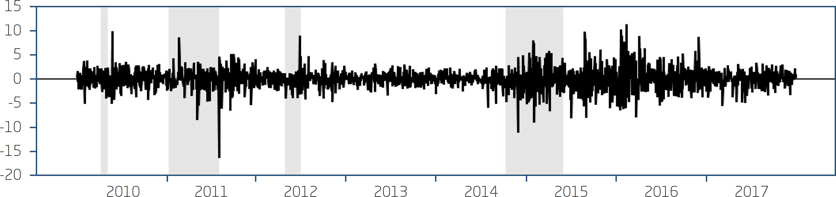
Under this matter, in order to identify the key events associated with extreme oil price movements, we selected the dates on which the return rate was greater than or equal to, in absolute value, 5%, as suggested by King, Deng, and Metz (2012). This variation occurred in only 3% of the cases, of which 46% were positive and 54% negative. Therefore, the emphasis is placed on data associated with large variations in the commodity returns and volatility clustering, which are the following highlighted in Figure 4.1:

Figure 4.1
DAILY WTI CRUDE OIL SPOT RETURN (2010-2017)

• April 2010: Deepwater Horizon offshore drilling unit explosion and Greek debt crisis.

• From December 2010 to April 2011: Arab Spring.

• June 2012: downgrade in the rating of major banks (Barclays, HSBC, Lloyds, Credit Suisse, Bank of America) by Moody’s.

• July 2015: sharp price drop of crude oil driven by growing supply, unwillingness of Opec members (Saudi Arabia, Iraq) to cut production, and the Iran nuclear deal with the United States, which removed economic sanctions from the Persian country.

Figure 4.1 displays some statistical properties of the data series, such as stochastic developments and non-constant volatility over time, that imply intermittent behaviour for the oil return with distinct periods of high and low volatility (clustering), which indicates the presence of some stylized facts related to financial series (Enders, 2008).

Figure 4.2 reports descriptive statistics of the data used in this work. Returns have an estimated mean close to zero, but standard deviations are high. It can also be noticed that skewness, kurtosis, and Jarque-Bera test values indicate a left asymmetric leptokurtic curve, characteristics that allow us to reject the null hypothesis of a normal curve as representative of the frequency distribution of oil return series. Therefore, those properties, as well as the high maximum and minimum values observed in all series, suggest the presence of jumps and variable volatility over time.

Figure 4.2
DESCRIPTIVE STATISTICS

Statistics	Value
Number of observations	2.008
Mean	0.026
Standard deviation	2.1126
Skewness	-0.0883
Kurtosis	4.3816
Jarque-Bera	p = 0.0000
ADF	p = 0.0000
Ljung-Box q-test	p = 0.6215
Ljung-Box q2-test	p = 0.0000
ARCH test	p = 0.0000

Source:

The ADF test score indicates that the oil return series are stationary, while the Ljung-Box q-test assesses the presence of autocorrelation in the series, which also suggests the presence of conditional heteroscedasticity on the square returns. We also applied the Lagrange multiplier diagnostic test proposed by Engle (1982) to assess the significance of ARCH effects on the return series, which indicates that the variance of the residuals is not constant across observations. All of the above results suggest that conditional heteroscedasticity models are better suited to describe the behaviour of oil returns, which are related to the findings of Gronwald (2012), Laurini et al. (2016), and Oliveira and Pereira (2017).

5. RESULTS

Estimates for the four extensions of the Chan and Maheu (2002) conditional jump model to the daily oil return (WTI) obtained through Equation 19 are given in figures 5.1 and 5.2. All extensions have included an autoregressive coefficient, a number defined by the Akaike information criterion, because it has higher efficiency and consistency than other alternative models. In general, the constant jump-intensity model shows worse results⁶, while ARJI - h_t specification, which uses a contemporary volatility forecast as an explanatory variable for the variance of the jump size, is the best one to describe the oil market behaviour, especially by allowing the jump distribution parameters to be time-varying and to eliminate correlation among observations.

Figure 5.1
CONSTANT AND TIME-VARYING JUMP-INTENSITY MODELS

Parameters	Constant	ARJI–GARCH
µ	0.0358 (0.0369)*	0.0277 (0.0391)*
ϕi	-0.0223 (0.0207)*	-0.0274 (0.0221)*
ϖ	0.0203 (0.0089)	0.0161 (0.0069)
α	0.0441 (0.0073)	0.0299 (0.0073)
β	0.9397 (0.0102)	0.9556 (0.0099)
ζ 0	4.2065 (0.8959)	4.1071 (0.73712)
η 0	-1.1590 (0.6001)	-0.6838 (0.5165)
λ 0	0.0403 (0.0190)	0.0283 (0.0126)
ρ		0.5086 (0.2049)
γ		0.5086 (0.2049)
Qξt(15)	21.41 {0.1242}	14.64 {0.4773}
Log-likelihood	-4057.6846	-4054.4405

• Standard errors are in parentheses, p-values of the Q test are in braces. The asterisk symbol denotes no significance at the 5% level.
Source:

Figure 5.2
ARJI-GARCH MODEL: JUMP INTENSITY

Figure 5.1 displays the estimates for both the constant and the autoregressive jump-intensity model. Regarding the GARCH parameters - ω, α e β - they are all statistically significant at the 5% level, indicating persistence and presence of a conditional variance process among oil price returns. This fact can be verified in Figure 4.1, which describes daily WTI oil returns from January 2010 to December 2017. There were severe oil price fluctuations, especially during the Arab Spring and the bank debt paper downgrade. Note that volatility in crude oil returns remained at a high level during these periods, while remaining relatively low in others. This is called volatility clustering. Therefore, the GARCH variance structure is appropriate for modelling this phenomenon (Gronwald, 2012; Oliveira & Pereira, 2017).

For both models, λ₀ and η₀ express the need for jump specification to describe oil market dynamics. The parameter λ₀ indicates that the mean of jumps in the constant model is 0.0403 and in the time-varying jump intensity is 0.0283, a fact that allows concluding that the second model is more adequate to capture jumps than the first specification. In turn, η₀ demonstrates that the conditional mean of the jump size is negative, i.e., sudden devaluations are more common than positive changes for the oil market, which is consistent with a negative asymmetry observed in the data (Figure 5.2). These results are similar to those reported in Askari and Krichene (2008) and Gronwald (2012).

Moreover, the ρ parameter in the ARJI-GARCH model, estimated to be 0.5086, suggests that the jump intensity is not persistent throughout the time and its constraint of equality to coefficient γ - a necessary condition for maximum likelihood estimation - suggests that unpredicted past shocks, ξ_t-1 have no influence on the probability of new jumps today.

The estimates for ζ₀ indicate that variations in jump intensity are high and well above the results obtained for stock market returns (Chan & Maheu, 2002; Qu & Perron, 2013) and exchange rate (Chan, 2004; Ely, 2013), results that are related to some other findings in the literature about the presence of high volatility in this market (Askari & Krichene, 2008; Oliveira & Pereira, 2017). Another issue to consider, the Ljung-Box Q_ξt (15) statistic, doesn’t reject the null hypothesis for independent and identically distributed (iid) residuals, that is, it eliminates the residual correlation of the ARMA (Equation 4) that sets the jump-intensity value.

Figure 5.2 presents the oil price level and the time-varying jump intensity, expressed by the λ_t parameter obtained from the estimated ARJI-GARCH model. It is observed that λ_t has an amplitude of around 0.7 jumps per day, characterized by low persistence and fast mean reversion to market volatility, besides presenting a certain regularity in the average number of jumps.

This paper presents a new contribution to this literature by allowing the conditional mean and conditional variance of the jump size distribution to be a function of past returns and GARCH volatility. Figure 5.3 presents estimates for both the constant and the autoregressive jump-intensity model ARJI - R²_t-1 and ARJI - h_t, respectively. Regarding the third specification, and η₀ are highly significant, but ζ₁ and η₁ are not, indicating that neither the variance nor the mean of the jump size accounts for past returns that can be justified by geopolitical issues, such as the reduction of price tension between Saudi Arabia and other Opec members and the decreasing US dependence on Middle Eastern oil imports.

Figure 5.3
ARJI - R²_{t - 1} AND ARJI - h_t MODELS

Parameters	ARJI - R2t-1	ARJI - ht
µ	0.0523 (0.0427)*	0.09298 (0.0470)*
ϕi	-0.0280 (0.0243)*	-0.0326 (0.0220)*
ϖ	0.0144 (0.0059)	0.0118 (0.0059)
α	0.0313 (0.0060)	0.0296 (0.0061)
β	0.9536 (0.0086)	0.9541 (0.0087)
ζ 0	3.2545 (0.7522)	-0.8344 (2.0782)*
ζ 1	0.0485 (0.1458)*	2.8784 (1.8105)*
η 0	-1.8806 (0.6018)	-1.7043 (0.4901)
η 1	0.3949 (0.2161)*	0.3668 (0.1941)*
η 2	-0.4832 (0.2396)	-0.3643 (0.1936)*
λ 0	0.0410 (0.0185)	0.0605 (0.0240)
ρ	0.4816 (0.1480)	0.4522 (0.1403)
γ	0.4816 (0.1480)	0.4522 (0.1403)
Qξt(15)	14.56 {0.374}	15.33 {0.0775}
Log-likelihood	-4050.9211	-4048.3419

• Note: Standard errors are in parentheses, p-values of the Q test are in braces. The asterisk symbol denotes no significance at the 5% level.
Source:

Figure 5.4 presents the time-varying jump intensity for the ARJI - R²_t-1 model, which has a maximum value about 22% higher than that obtained for the ARJI-GARCH specification, providing a more accurate fit to the data and more significant impacts of extreme events on oil price volatility. However, it presents similar characteristics related to low persistence and regularity in the jump intensity, especially in moments that have a huge impact on the oil industry, such as the Deepwater Horizon offshore drilling unit explosion and the Arab Spring (Laurini et al., 2016).

Figure 5.4
ARJI-R²_t-1: JUMP INTENSITY

The estimated values for the last extension, ARJI - h_t, suggest that this is the best model that fits the data⁷, which allows the conditional jump intensity to evolve according to an ARMA process. The statistical significance for both λ₀ and ρ parameters meets the evidence found in previous specifications, besides allowing the conditional variance of the jump size to be exclusively a function of estimated volatility (ζ₁)

Once again, η₀ < 0 suggests that jumps are responsible for a rapid reversion to the average level of oil market volatility, although the model does not capture any time dynamics. Intuitively, this suggests that negative oil price shocks generate higher volatility on the global light oil market than positive ones, which is in contrast to the efficient market hypothesis. However, this effect is quickly absorbed by product prices, meeting the evidence provided by Bagchi (2017) and Oliveira and Pereira (2017).

Figure 5.5 suggests that the jump intensity for the ARJI - h_t specification is similar ARJI - R_2t-1 to model results, also reporting a maximum amplitude of one jump per day and increases in the average quantity of expected jumps at critical moments, especially during environmental disasters and wars, but with small differences at moments of higher stabilities when compared to the last model.

Figure 5.5
MODEL ARJI - h_t: JUMP INTENSITY

In order to show how variations in the estimated value of λ_t have important consequences on the Poisson distribution, which describes the number of jumps that arrive between periods t - 1 and t, Figure 5.6 plots theoretical probabilities of the occurrence of jumps for the constant jump-intensity model and ARJI - h_t specification for two different dates on which the commodity suffered severe movements in its price: April 20th, 2010 (Deepwater Horizon offshore drilling unit explosion) and June 18th, 2012 (downgrade of bank ratings).

Figure 5.6
PROBABILITY OF JUMPS: CONSTANT MODEL × ARJI - h_t

This graphic shows that small changes in λ_t can have important effects on forecasting the probability of jumps at the suggested dates, and it is clearly evident that the risk associated with the realization of jumps in the constant-intensity model is considerably less than in the ARJI - h_t specification. The last model estimated a probability of about 15% for at least one jump following the environmental accident and 7% due to the downgrade of international banks; however, in the constant-intensity model, the probability is negligible at both times. Hence, such results reinforce the insights presented by Hamilton (2011), Kilian (2014), and Laurini et al. (2016) about the importance of extreme events not to be directly linked to industry pricing strategies, mainly because oil demand is highly inelastic in the short term.

Figure 5.7 displays predictive λ for the entire month of June 2012. It can be noticed that there was a considerable increase in the likelihood of a jump in two periods: June 2nd - 5th and June 20th - 25th. At both moments, this effect dissipates rapidly, reflecting a mean reversal in the series volatility. Moreover, it can also be seen that, at the time of the Moody’s bank credit downgrade, there was an increase in the average intensity of jumps, rising from 0.509 at the first jump to 0.554, when the second jump occurred, that is, an increase of approximately 10% in jump strength.

Figure 5.7
EFFECTS OF BANKING DOWNGRADE AT CONDITIONAL JUMP INTENSITY

Here, jumps occur in the context of bringing the return rate towards its historical mean followed by a period of certain stability; additionally, the greater the number of jumps within a relatively short time window, the stronger the intensity of the effect caused by the subsequent jump compared to the one caused by the previous jump, but with a smoother descending path.

6. CONCLUDING REMARKS

According to the literature, jumping models have proven to be a useful tool for dealing with extreme events and sudden price chances, and in addition they have been successfully applied to various types of financial market variables. This paper examined the jump dynamics on the light oil price return (WTI) for the period from January 2010 to December 2017 through four specifications of conditional jump model proposed by Chan and Maheu (2002) and found strong evidence for the GARCH behaviour of the jump intensity variable in time.

Consequently, we argue that the oil market is highly susceptible to the reception of new information and the occurrence of extreme events, so that oil price reactions tend to vary with different political and economic events and environmental disasters. According to figures 5.2, 5.4, and 5.5, the intensity of the jump in global oil prices peaked at the end of the Arab Spring in July 2011, and another big jump occurred in April 2010, when the Deepwater Horizon platform exploded. This demonstrates that the crude oil market experienced drastic ups and downs during the year and especially that sudden negative shocks create higher volatility in oil markets than do positive shocks. Between 2010 and 2017, shocks caused by production factors seem smaller but happened more frequently in comparison to shocks driven by geopolitical and environmental factors.

Regarding the econometric results, it was found that the ARJI - h_t model is superior to others in terms of adherence data, which is confirmed by the value of the log-likelihood and the significance of the parameter ζ₁ in a scenario of environmental disasters and geopolitical and financial crises. In addition, the jump intensity coefficients (ρ, γ) indicate that the jumps in oil returns follow a first-order autoregressive process and that it is reasonable to use the ARJI parameterization. The estimate of ρ is close to 0.4, implying a low degree of persistence in the intensity of the jump, and the average size of the jumps is negative (η₀), suggesting that the jumps are responsible for the reversal of the average market volatility, in addition to not presenting a temporal dynamic.

The analysis of the reduction in credit bond ratings of large banks in June 2012, Figure 5.7, confirms that the intensity of the jumps is directly related to market volatility. However, when the jump size variance is allowed to be a function of the predicted volatility, a smaller number of jumps explains the variation in oil prices, and over a short period of time the average intensity of subsequent jumps is greater than that indicated by the model’s predecessor, besides presenting a smoother decay.

Intuitively, the occurrence of extreme events causes significant short-term changes. However, this effect is quickly absorbed by product prices. In this sense, the main contribution of this paper is to present an econometric framework that addresses the nature of the stochastic process underlying oil prices and the importance of components that drive this process, as well as to explain why investors, policymakers, and producers can consciously decide not to make hedges against extreme events, especially if there are informational costs for learning the structures that govern them.

The limitations of this research are threefold: none of the proposed specifications consider the problem of mutual dependence on the volatility and intensity of the unexpected event (jump); despite the finding that there are evident asymmetries between good and bad news in the market, this difference has not been quantified; and because of the evidence that the effects of extreme events last for the short term, it is necessary to use tick-by-tick data to examine its real impact over the volatility of oil returns.

For future research, it is recommended that investigators study the short and long-term relationship in the oil market context, as the omission of structural changes in the price level may lead to spurious statistical results, forecasting errors and insecurity about the specified model. Further studies are also recommended on the relationship, externalities, and response time of abrupt effects on commodities over the stock market and macroeconomic variables in the context of national economies, such as inflation, interest rates, and income.

• 3
  For the purpose of this paper, we use the definition of volatility proposed by Bollerslev (1986): ${\mathit{\sigma }}_{\mathit{t}}^2=\mathit{\omega }+{\mathit{\alpha }\epsilon }_{\mathit{t}-1}^2+{\mathit{\beta }\mathit{\sigma }}_{\mathit{t}-1}^2;\mathit{\alpha }>0,\mathit{\beta }>0,\mathit{\alpha }+\mathit{\beta }<1$, where α and β are referred to as ARCH and GARCH parameters, respectively.
• 4
  Low-frequency events with high magnitude that are concentrated in the tails of the distribution function that fits the data series under analysis (Rocco, 2014). Finanças Estratégicas
• 5
  Probabilistic distribution, commonly used to model the frequency of occurrences of an event over a period of time or space.
• 6
  Smaller log-likelihood value.
• 7
  To verify the robustness of the ARJI - h_t model in relation to the estimated persistence of shocks (ρ) and conditional heteroscedasticity in oil prices, estimates were made for subsamples referring to periods of higher volatility, which were defined based on the data behaviour. The subsample periods are from 03/01/2010 to 10/01/2010; from 01/01/2011 to 31/12/2011; from 03/01/2012 to 11/01/2012; and from 01/07/2014 to 28/02/2016. In all situations, the GARCH parameters were significant and the values for ρ were similar.

REFERENCES

• Andersen, T. G., Bollerslev, T., & Diebold, F. X. (2007). Roughing it up: Including jump components in the measurement, modeling, and forecasting of return volatility. The Review of Economics and Statistics, 89(4), 701-720. doi:10.1162/rest.89.4.701
  » https://doi.org/10.1162/rest.89.4.701
• Askari, H., & Krichene, N. (2008). Oil price dynamics (2002-2006). Energy Economics, 30(5), 2134-2153. doi:10.1016/j.eneco.2007.12.004
  » https://doi.org/10.1016/j.eneco.2007.12.004
• Bagchi, B. (2017). Volatility spillovers between crude oil price and stock markets: Evidence from BRIC countries. International Journal of Emerging Markets, 12, 352-365. doi:10.1108/IJoEM-04-2015-0077
  » https://doi.org/10.1108/IJoEM-04-2015-0077
• Bollerslev, T. (1986). Generalized autoregressive conditional heteroskedasticity. Journal of Econometrics, 31(3), 307-327. doi:10.1016/0304-4076(86) 90063-1
  » https://doi.org/10.1016/0304-4076(86) 90063-1
• Chan, W. H. (2004). Conditional correlated jump dynamics in foreign exchange. Economics Letters, 83(1), 23-28. doi:10.1016/j.econlet.2003. 09.023
  » https://doi.org/10.1016/j.econlet.2003. 09.023
• Chan, W. H., & Maheu, J. M. (2002). Conditional jump dynamics in stock market returns. Journal of Business & Economic Statistics, 20(3), 377-389. doi:10.1198/073500102288618513
  » https://doi.org/10.1198/073500102288618513
• Chan, W. H., & Young, D. (2006). Jumping hedges: An examination of movements in copper spot and futures markets. Journal of Futures Markets, 26(2), 169-188. doi:10.1002/fut.20190
  » https://doi.org/10.1002/fut.20190
• Chiou, J., & Lee, Y. (2009). Jump dynamics and volatility: Oil and the stock markets. Energy, 34(6), 788-796. doi:10.1016/j.energy.2009.02.011
  » https://doi.org/10.1016/j.energy.2009.02.011
• Ely, R. A. (2013). Dinâmica dos saltos condicionais na taxa de câmbio brasileira. Revista Brasileira de Economia de Empresas, 13(1), 59-75. Retrieved from https://portalrevistas.ucb.br/index.php/rbee/article/view/4251
  » https://portalrevistas.ucb.br/index.php/rbee/article/view/4251
• Enders, W. (2008). Applied econometric time series New York: John Wiley & Sons.
• Engle, R. F. (1982). A general approach to Lagrange multiplier model diagnostics. Journal of Econometrics, 20(1), 83-104. doi:10.1016/0304-4076 (82)90104-X
  » https://doi.org/doi:10.1016/0304-4076 (82)90104-X
• Gronwald, M. (2009). Jumps in oil prices - evidence and implications [Working Paper n. 75]. Ifo Institute, Leibniz Institute for Economic Research at the University of Munich, Munich. Retrieved from https://www.econstor.eu/bitstream/10419/73779/1/IfoWorkingPaper-75.pdf
  » https://www.econstor.eu/bitstream/10419/73779/1/IfoWorkingPaper-75.pdf
• Gronwald, M. (2012). A characterization of oil price behavior? Evidence from jump models. Energy Economics, 34(5), 1310-1317. doi:10.1016/j.eneco.2012.06.006
  » https://doi.org/10.1016/j.eneco.2012.06.006
• Hamilton, J. D. (2008). Understanding crude oil prices [Working Paper n. 14492]. National Bureau of Economic Research, Cambridge, MA. doi:10. 3386/w14492
  » https://doi.org/10. 3386/w14492
• Hamilton, J. D. (2011). Historical oil shocks [Working Paper n. 6790]. National Bureau of Economic Research, Cambridge, MA. Retrieved from https://www.nber.org/papers/w16790.pdf
  » https://www.nber.org/papers/w16790.pdf
• Horan, S. M., Peterson, J. H., & Mahar, J. (2004). Implied volatility of oil futures options surrounding OPEC meetings. The Energy Journal, 25(3), 103-125. doi:10.5547/ISSN0195-6574-EJ-Vol25-No3-6
  » https://doi.org/10.5547/ISSN0195-6574-EJ-Vol25-No3-6
• Hotelling, H. (1931). The economics of exhaustible resources. The Journal of Political Economy, 39(2), 137-175. doi:10.1086/254195
  » https://doi.org/10.1086/254195
• Kilian, L. (2014). Oil price shocks: Causes and consequences. Annual Review of Resource Economics, 6(1), 133-154. doi:10.1146/annurev-resource-083 013-114701
  » https://doi.org/10.1146/annurev-resource-083 013-114701
• Kim, H. Y., & Mei, J. P. (2001). What makes the stock market jump? An analysis of political risk on Hong Kong stock returns. Journal of International Money and Finance, 20(7), 1003-1016. doi:10.1016/S0261-5606(01)00035-3
  » https://doi.org/10.1016/S0261-5606(01)00035-3
• King, K., Deng, A., & Metz, D. (2012). An econometric analysis of oil price movements: The role of political events and economic news, financial trading, and market fundamentals. Bates White Economic Consulting. Retrieved from https://www.bateswhite.com/media/pnc/4/media.444.pdf
  » https://www.bateswhite.com/media/pnc/4/media.444.pdf
• Larsson, K., & Nossman, M. (2011). Jumps and stochastic volatility in oil prices: Time series evidence. Energy Economics, 33(3), 504-514. doi:10.10 16/j.eneco.2010.12.016
  » https://doi.org/10.10 16/j.eneco.2010.12.016
• Laurini, M. P., & Mauad, R. B. (2015). A common jump factor stochastic volatility model. Finance Research Letters, 12, 2-10. doi:10.1016/j.frl.2014. 12.009
  » https://doi.org/10.1016/j.frl.2014. 12.009
• Laurini, M. P., Mauad, R., & Aiube, F. A. L. (2016). Multivariate stochastic volatility-double jump model: An application for oil assets [Working Paper n. 415]. Banco Central do Brasil, Brasília. doi:10.2139/ssrn.3037158
  » https://doi.org/10.2139/ssrn.3037158
• Lobo, B. J. (1999). Jump risk in the US stock market: Evidence using political information. Review of Financial Economics, 8(2), 149-163. doi:10.1016/S10 58-3300(00)00011-2
  » https://doi.org/10.1016/S10 58-3300(00)00011-2
• Maheu, J. M., & McCurdy, T. H. (2004). News arrival, jump dynamics, and volatility components for individual stock returns. The Journal of Finance, 59(2), 755-793. doi:10.1111/j.1540-6261.2004.00648.x
  » https://doi.org/10.1111/j.1540-6261.2004.00648.x
• Morales, L., & Andreosso-O’Callaghan, B. (2017). Volatility in agricultural commodity and oil markets during times of crises. Economics, Management & Financial Markets, 12(4), 59-82. doi:10.22381/EMFM 12420173
  » https://doi.org/10.22381/EMFM 12420173
• Oliveira, A. B., & Pereira, P. L. V. (2017). Mudança de regime e efeito ARCH em volatilidade: Um estudo dos choques das cotações do Petróleo. Revista Brasileira de Finanças, 15(2), 197-225. Retrieved from http://www.redalyc.org/pdf/3058/305855642002.pdf
  » http://www.redalyc.org/pdf/3058/305855642002.pdf
• Ozdemir, Z. A., Gokmenoglu, K., & Ekinci, C. (2013). Persistence in crude oil spot and futures prices. Energy, 59, 29-37. doi:10.1016/j.energy.2013. 06.008
  » https://doi.org/10.1016/j.energy.2013. 06.008
• Pindyck, R. S. (2001). The dynamics of commodity spot and futures markets: A primer. The Energy Journal, 22(3), 1-29. Retrieved from https://www.jstor.org/stable/41322920
  » https://www.jstor.org/stable/41322920
• Press, S. J. (1967). A compound events model for security prices. Journal of Business, 40(3), 317-335. Retrieved from https://www.jstor.org/stable/2351754
  » https://www.jstor.org/stable/2351754
• Qu, Z., & Perron, P. (2013). A stochastic volatility model with random level shifts and its applications to S&P 500 and NASDAQ return indices. The Econometrics Journal, 16(3), 309-339. doi:10.1111/j.1368-423X.2012. 00394.x
  » https://doi.org/10.1111/j.1368-423X.2012. 00394.x
• Rocco, M. (2014). Extreme value theory in finance: A survey. Journal of Economic Surveys, 28(1), 82-108. doi:10.1111/j.1467-6419.2012.00744.x
  » https://doi.org/10.1111/j.1467-6419.2012.00744.x
• Sadorsky, P. (1999). Oil price shocks and stock market activity. Energy Economics, 21(5), 449-469. doi:10.1016/S0140-9883(99)00020-1
  » https://doi.org/10.1016/S0140-9883(99)00020-1

Publication Dates

• Publication in this collection
  30 Mar 2020
• Date of issue
  2020

History

• Received
  29 Apr 2019
• Accepted
  22 Aug 2019