Surface charges and external electric field in a toroid carrying a steady current

Surface charges and external electric field in a toroid carrying a steady current

J. A. Hernandes; A. K. T. Assis

Instituto de Física 'Gleb Wataghin', Universidade Estadual de Campinas - Unicamp 13083-970 Campinas, São Paulo, SP, Brasil

ABSTRACT

We solve the problem of a resistive toroid carrying a steady azimuthal current. We use standard toroidal coordinates, in which case Laplace's equation is R-separable. We obtain the electric potential inside and outside the toroid, in two separate cases: 1) the toroid is solid; 2) the toroid is hollow (a toroidal shell). Considering these two cases, there is a difference in the potential inside the hollow and solid toroids. We also present the electric field and the surface charge distribution in the conductor due to this steady current. These surface charges generat not only the electric field that maintains the current flowing, but generate also the electric field outside the conductor. The problem of a toroid is interesting because it is a problem with finite geometry, with the whole system (including the battery) contained within a finite region of space. The problem is solved in an exact analytical form. We compare our theoretical results with an experimental figure demonstrating the existence of the electric field outside the conductor carrying steady current.

1 Toroidal Ring

The electric field outside conductors with steady currents has been studied in a number of cases. These cases, however, consider infinitely long conductors: coaxial cable, [1, pp. 125-130], [2, pp. 318 and 509-511], [3], [4, pp. 336-337] and [5]; solenoid with azimuthal current, [2, p. 318] and [6]; transmission line, [7, p. 262] and [8]; straight wire, [9]; and conductor plates, [10]. The only cases solved in the literature where the geometry of the conductor is finite are those of a finite coaxial cable considered by Jackson, [11], and that of a toroidal conducting ring, [12].

Here we consider the case of the conducting toroid with a steady current. Our goal is to find the electric potential inside and outside the toroid, and from the potential we can find the electric field and surface charges. More details about this problem and its analytical solution can be found in [12].

Consider a toroidal conductor with uniform resistivity. It has greater radius R₀ and smaller radius r₀ and carries a steady current I in the azimuthal direction, flowing along the circular loop. The toroid has rotational symmetry around the z-axis and is centered in the plane z = 0. The battery that maintains the current is located at j = p rad, see Fig. 1. Air or vacuum surrounds the conductor.

The electric potential f can be calculated using toroidal coordinates (h, x, j) [13, p. 112], defined by:

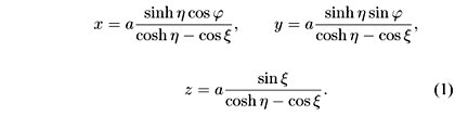
Here, a is a constant such that when h ® ¥ we have the circle x = acosj, y = asinj and z = 0. The toroidal coordinates can have the possible values: 0 < h < ¥, -p rad < x < p rad and -p rad < j < p rad. We take h₀ as a constant that described the toroid surface in toroidal coordinates. The internal (external) region of the toroid is characterized by h > h₀ (h < h₀).

The potential along the surface of the toroid is linear in j, f(h₀, x, j) = A + Bj. This potential can be expanded in Fourier series in j:

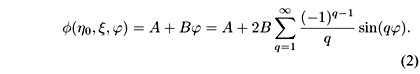
Eq. (2) can be used as the boundary condition for our particular solution to this problem.

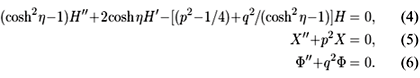
Laplace's equation for the electric potential Ѳf = 0 can be solved in toroidal coordinates with the method of separation of variables (by a procedure known as R-separation), leading to a solution of the form, [13, p. 112]:

where the functions H, X, and F satisfy the general equations (where p and q are constants):

Using the boundary condition (2) and the possible solutions of Eqs. (4) to (6) we obtain the potential as given by, [12]:

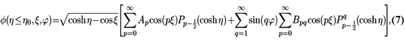
where the coefficients A_p and B_pq are given by, respectively:

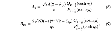
where d_wp is the Kronecker delta, which is zero for w ¹ p and one for w = p. The functions (cosh h) and (cosh h) are known as toroidal Legendre polynomials of the first and second kind respectively, [14, p. 173].

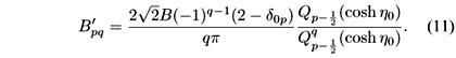
For the region inside the hollow toroid (that is, h > h₀), the potential is given by:

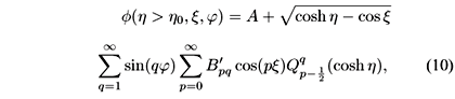
where the coefficients are defined by:

We plotted the equipotentials of a full solid toroid on the plane z = 0 in Fig. 2 with A = 0 and B = f₀/2p. Fig. 3 shows a plot of the equipotentials of the full solid toroid in the plane x = 0 (perpendicular to the current).

2 Electric Field and Surface Charges

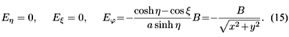
The electric field can be calculated by = -Ñf in toroidal coordinates, as given by:

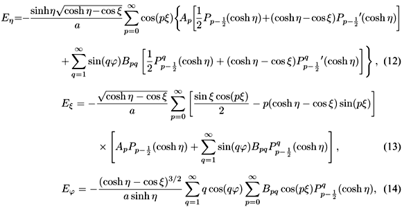
where

^¢(cosh h) are the derivatives of the (cosh h) relative to cosh h. The electric field inside the full solid toroid (h > h₀) is given simply by:

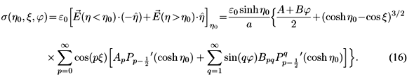
For the full solid toroid, the surface charge distribution that creates the electric field inside (and outside of) the conductor, keeping the current flowing, can be obtained with Gauss' law (by choosing a Gaussian surface involving a small portion of the conductor surface):

3 Thin Toroid Approximation

Here we treat the case of a thin toroid, such that the outer radius R₀ = acosh h₀/sinh h₀» a and the inner radius r₀ = a/sinh h₀ are related by r₀ << R₀, see Fig. 1. In this case we have cosh h₀ >> h₀ >> 1. The function (cosh h₀) that appears in Eqs. (8) and (9) for the coefficients A_p and B_pq can be approximated by, [14, p. 164]:

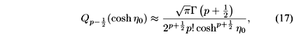
where G is the gamma function, [15, p. 591].

Because Eq. (17) has a factor of cosh^-p- h₀ << 1, we can neglect all terms with p > 0 in Eq. (7) compared with the term with p = 0. The potential outside the thin toroid (h₀ >> 1):

We are especially interested in the expressions for the potential and electric field outside but in the vicinity of the conductor, h₀ > h >> 1. A series expansion of the functions (x) and ¢(x) around x ® ¥ gives as the most relevant terms [14, p. 173]:

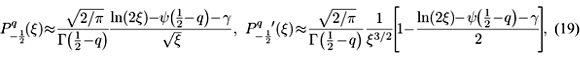
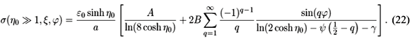
where y(z) = G¢(z)/G(z) is the digamma function, and g » 0.577216 is the Euler gamma. The potential just outside the thin toroid, Eq. (7), can then be written in this approximation as:

This is a new result not presented in [12].

Far from the battery (that is, for |j| << p rad) the potential (20) can be fitted numerically by trial and error by the following simpler expression (valid for h₀ > 10³):

This is a correction from Eq. (35) of [12].

The surface charge distribution in this thin toroid approximation is given by:

This is another new result not presented in [12]. In Fig. 4 we plotted the density of surface charges s as a function of the azimuthal angle j. We can see that s is linear with j only close to j = 0 rad. Close to the battery s diverges to infinity (that is, s ® ¥ when j ® ±p rad).

Far from the battery Eq. (22) can be fitted numerically by a linear function on j, namely:

This is a correction from Eq. (37) of [12]. We defined s_A and s_B by this last equality.

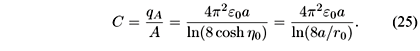
We can calculate the total charge q_A of the thin toroid as a function of the constant electric potential A. For this, we integrate the surface charge density s, Eq. (22), in x and j (in the approximation cosh h₀ >> 1):

where h_h = h_x = a/(cosh h - cos x) and h_j = a sinh h/(cosh h - cos x) are the scale factors in toroidal coordinates, [16]. Notice that from Eq. (24) we can obtain the capacitance of the thin toroid, [17, p. 127]:

It is useful to define a new coordinate system:

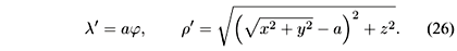
We can interpret l¢ as a distance along the toroid surface in the j direction, and r¢ as the shortest distance from the circle x² + y² = a² located in the plane z = 0. Consider a certain piece of the toroid between the angles j₀ and -j₀, with potentials in these extremities given by f_R = A + Bj₀ and f_L = A - Bj₀, respectively. This piece has a length of = 2aj₀. When h₀ > h >> 1 (that is, r₀ < r¢ << a) the potential can be written as:

where in the last approximation we neglected the term ln(/a) utilizing the approximation r₀ < r¢ << a (so that /r₀ > /r¢ >> /1.67a > /8a). The electric field can be expressed in this approximation as:

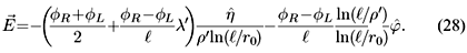
Eqs. (27) and (28) can be compared to Eqs. (12) and (13) of Assis, Rodrigues and Mania, [9], respectively. They have studied the case of a long straight cylindrical conductor of radius r₀ carrying a constant current, in cylindrical coordinates (r¢, j, z) (note that the conversions from toroidal to cylindrical coordinates in this approximation are » -¢ and » ). In their case, the cylinder has a length and radius r₀ << , with potentials f_L and f_R in the extremities of the conductor, and RI = f _L - f_R. Our result of the potential in the region close to the thin toroid coincides with the cylindrical solution, as expected.

4 Charged Toroid Without Current

Consider a toroid described by h₀, without current but charged to a constant potential f₀. Using A = f₀ and B = 0 in Eqs. (7) we have the potential inside and outside the toroid, respectively:

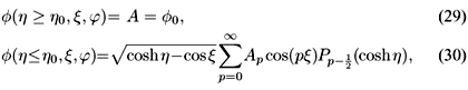
where the coefficients A_p are given by Eq. (8). This solution is already known in the literature, [18, p. 239], [19, p. 1304].

It is also possible to obtain the capacitance of the toroid, by comparing the electrostatic potential at a distance r far from the origin with the potential given by a point charge q, f(r >> a) » q/4pe₀r:

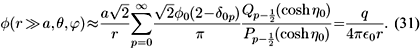
The capacitance of the toroid with its surface at a constant potential f₀ can be written as C = q/f₀. From Eq. (31) this yields, [18, p. 239], [20, p. 5-13], [21, p. 9], [22, p. 375]:

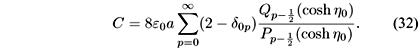
Utilizing the thin toroid approximation, h₀ >> 1, one can obtain the capacitance of a circular ring, Eq. (25).

Another case of interest is that of a charged circular line discussed below, which is the particular case of a toroid with r₀ ® 0. With h₀ >> 1 and cosh h₀ >> 1 we have R » a. Keeping only the term with p = 0 in Eqs. (8) and (30), expressed in toroidal and spherical coordinates (r, q, j) respectively, the potential for the thin toroid becomes:

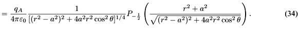
We can expand Eq. (34) on r _< /r _> , where r _< (r _> ) is the lesser (greater) between a and r = . We present the first three terms:

Eqs. (33) to (35) can be compared with the solution given by Jackson, [23, p. 93]. Jackson gives the exact electrostatic solution of the problem of a charged circular wire (that is, a toroid with radius r₀ = 0), in spherical coordinates (r, q, j):

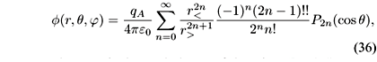
where q_A is the total charge of the wire. Eq. (36) expanded to n = 2 yields exactly Eq. (35). We have checked that Eqs. (34) and (36) are the same for at least n = 30.

Eqs. (33) and (36) yield the same result. It is worthwhile to note that in spherical coordinates we have an infinite sum, Eq. (36), while in toroidal coordinates the solution is given by a single term, Eq. (34). The agreement shows that Eqs. (33) and (36) are the same solution only expressed in different forms.

Figure 5 shows the potential as function of r (in cylindrical coordinates) in the plane z = 0. Eqs. (33) and (36) give the same result.

5 Discussion and Conclusion

Figure 2 can be compared with the experimental result found by Jefimenko, [24, Fig. 3], reproduced here in Fig. 6 with Fig. 2 overlaid on it. Jefimenko painted a circular conducting strip on a glass plate utilizing a transparent conducting ink. A steady current flowed in the strip by connecting its extremities with a battery. By spreading grass seeds on the glass plate he was able to map the electric field lines inside and outside the strip (in analogy with iron fillings mapping the magnetic field lines). The equipotential lines obtained here are orthogonal to the electric field lines. There is a very reasonable agreement between our theoretical result and the experiment.

Our solution inside and along the surface of the full solid toroid yields only an azimuthal electric field, namely, |E_j| = Df/2pr. But even for a steady current we must have a component of pointing away from the z axis, E_r, due to the curvature of the wire. Here we are neglecting this component due to its extremely small order of magnitude compared with the azimuthal component E_j. See further discussion in [12].

The beautiful experimental result of Jefimenko showing the electric field outside the conductor is complemented by this present theoretical work, with excellent agreement, Figs. 6. The electric potential and electric field of the thin toroid approximation with a steady current, respectively Eqs. (27) and (28), agree with the known case of a long straight cylindrical conductor carrying a steady current, Eqs. (12) and (13) of [9]. The electric potential of the thin toroid approximation without current agrees with the known result of a charged wire, [23, p. 93].

Here we have obtained a theoretical solution for the potential due to a steady azimuthal current flowing in a toroidal resistive conductor which yielded an electric field not only inside the toroid but also in the space surrounding it. Our solution showed a reasonable agreement with Jefimenko's experiment which proved the existence of this external electric field due to a resistive steady current.

Acknowledgments

The authors wish to thank Fapesp (Brazil) for financial support to DRCC/IFGW/Unicamp in the past few years. They thank Drs. R. A. Clemente and S. Hutcheon for relevant comments, references and suggestions. One of the authors (JAH) wishes to thank CNPq (Brazil) for financial support.

Received on 2 February, 2004; revised version received on 7 May, 2004

• [1] A. Sommerfeld, Electrodynamics (Academic Press, New York, 1964).
• [2] O. D. Jefimenko, Electricity and Magnetism (Electret Scientific Company, Star City, 1989), 2nd ed.
• [3] A. K. T. Assis and J. I. Cisneros, in Open Questions in Relativistic Physics, edited by F. Selleri (Apeiron, Montreal, 1998), pp. 177-185.
• [4] D. J. Griffiths, Introduction to Electrodynamics (Prentice Hall, New Jersey, 1999), 3rd ed.
• [5] A. K. T. Assis and J. I. Cisneros, IEEE Trans. Circ. Sys. I 47, 63 (2000).
• [6] M. A. Heald, Am. J. Phys. 52, 522 (1984).
• [7] J. A. Stratton, Electromagnetic Theory (McGraw-Hill, New York, 1941).
• [8] A. K. T. Assis and A. J. Mania, Rev. Bras. Ens. Fís. 21, 469 (1999).
• [9] A. K. T. Assis, W. A. Rodrigues Jr. and A. J. Mania, Found. Phys. 29, 729 (1999).
• [10] A. K. T. Assis, J. A. Hernandes, and J. E. Lamesa, Found. Phys. 31, 1501 (2001).
• [11] J. D. Jackson, Am. J. Phys. 64, 855 (1996).
• [12] J. A. Hernandes and A. K. T. Assis, Phys. Rev. E 68, 046611 (2003).
• [13] P. Moon and D. E. Spencer, Field Theory Handbook(Springer-Verlag, Berlin, 1988), 2nd ed.
• [14] H. Bateman, Higher Transcendental Functions, vol. 1 (McGraw-Hill, New York, 1953).
• [15] G. B. Arfken and H. J. Weber, Mathematical Methods for Physicists (Academic Press, San Diego, 1995), 4th ed.
• [16] E. Ley-Koo and A. Góngora T., Rev. Mex. Fís. 40, 805 (1994).
• [17] E. Weber, Electromagnetic Fields: Theory and Applications, vol. 1 (John Wiley & Sons, New York, 1950).
• [18] W. R. Smythe, Static and Dynamic Electricity (Hemisphere, New York, 1989).
• [19] P. M. Morse and H. Feshback, Methods of Theoretical Physics, vol. 2 (McGraw-Hill, New York, 1953).
• [20] D. E. Gray, American Institute of Physics Handbook (McGraw-Hill, New York, 1972).
• [21] C. Snow, Formulas for Computing Capacitance and Inductance (Department of Commerce, Washington, 1954).
• [22] P. Moon and D. E. Spencer, Field Theory for Engineers (D. Van Nostrand Company, Princeton, New Jersey, 1961).
• [23] J. D. Jackson, Classical Electrodynamics (John Wiley, New York, 1999), 3rd ed.
• [24] O. D. Jefimenko, Am. J. Phys. 30, 19 (1962).

Publication Dates

• Publication in this collection
  01 Mar 2005
• Date of issue
  Dec 2004

History

• Received
  02 Feb 2004
• Accepted
  07 May 2004