Figure 1:
Original signal with upper and lower push and first step of mean value Huang and Shen, (2005Norden E Huang, Samuel S P Shen, (2005) Hilbert-Huang Transform and Its Applications, World Scientific Publishing Co. Pte. Ltd Volume 5).
Figure 2:
Original signal with first step difference with mean value Huang and Shen, (2005Norden E Huang, Samuel S P Shen, (2005) Hilbert-Huang Transform and Its Applications, World Scientific Publishing Co. Pte. Ltd Volume 5).
Figure 3:
The result of first step sifting process Huang and Shen, (2005Norden E Huang, Samuel S P Shen, (2005) Hilbert-Huang Transform and Its Applications, World Scientific Publishing Co. Pte. Ltd Volume 5).
Figure 4:
Original signal with first step residual Huang and Shen, (2005Norden E Huang, Samuel S P Shen, (2005) Hilbert-Huang Transform and Its Applications, World Scientific Publishing Co. Pte. Ltd Volume 5).
Figure 5:
Numerical test signal generated in MATLAB software.
Figure 6:
First cluster decomposed IMF's of numerical test in different frequencies a: 400Hz, b: 200Hz and c: 40Hz.
Figure 7:
the second cluster of IMFs (a, b and c) and general trend (d).
Figure 8:
a: numerical test signal, b: noise, c: noisy numerical test signal and d: magnified comparison of noisy and pure numerical test signal.
Figure 9:
Noise effect on EMD, all first IMF to sixth IMF's are noise in a, b, c, d, e and f, respectively.
Figure 10:
Decomposition of a: first IMF, b: second IMF, c: third IMF and d: fourth IMF.
Figure 11:
FFT spectrum of a: first IMF, b: second IMF, c: third IMF and d: fourth IMF.
Figure 12:
Locations of gears and bearings on input shaft (upper side) and output shaft (lower side).
Figure 13:
Applied engine map for simulation.
Figure 14:
Locations of accessible bearing for data acquisition on simple model.
Figure 15:
Boundary condition for static simulation for choosing mesh length.
Figure 16:
Static simulation result of input gear for mesh independency.
Figure 17:
Convergence of mesh length of mesh independency.
Figure 18:
Meshed model of input gear with length of 0.5 mm.
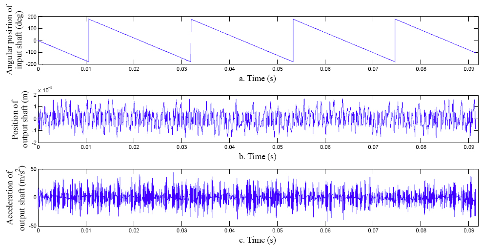
Figure 19:
a: angular position, b: position and c: acceleration of input shaft.
Figure 20:
a: Noisy no faulty signal and b: noisy no faulty signal in comparison of pure no faulty signal of input shaft.
Figure 21:
Input faulty gear.
Figure 22:
a: angular position, b: Position and c: acceleration of faulty input shaft.
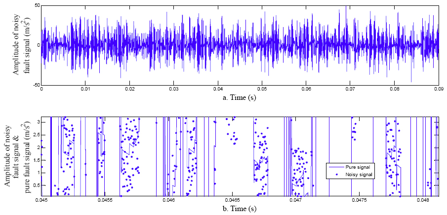
Figure 23:
a: Noisy faulty signal and b: noisy faulty signal in comparison of pure faulty signal of faulty input shaft.
Figure 24:
Input partial faulty gear.
Figure 25:
a: angular position, b: Position and c: acceleration of partial faulty input shaft.
Figure 26:
a: Noisy partial faulty signal and b: noisy partial faulty signal in comparison of pure partial faulty signal of faulty input shaft.
Figure 27:
Butterworth low pass filter phase and magnitude in linear system.
Figure 28:
a: zoomed and b: un-zoomed filtered no faulty signal.
Figure 29:
FFT spectrum of no faulty filtered signal.
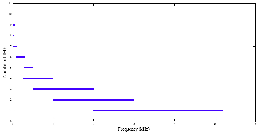
Figure 30:
Range of FFT spectrum of each IMF in frequency axis.
Figure 31:
a: first IMF, b: second IMF, c: third IMF and d: fourth IMF of no faulty signal.
Figure 32:
FFT spectrum of a: first IMF, b: second IMF, c: third IMF and d: fourth IMF of no faulty signal.
Figure 33:
a: zoomed and b: un-zoomed filtered one teeth faulty signal.
Figure 34:
FFT spectrum of one teeth faulty filtered signal.
Figure 35:
a: first IMF, b: second IMF, c: third IMF and d: fourth IMF of one teeth faulty signal.
Figure 36:
FFT spectrum of a: first IMF, b: second IMF, c: third IMF and d: fourth IMF of one teeth faulty signal.
Figure 37:
a: filtered signal, b: second IMF and c: FFT spectrum of second IMF of partial faulty signal.