Structural dynamic analysis for time response of bars and trusses using the generalized finite element method

Structural dynamic analysis for time response of bars and trusses using the generalized finite element method

André Jacomel Torii^*; Roberto Dalledone Machado

Graduate Program in Numerical Methods in Engineering (PPGMNE), Federal University of Paraná (UFPR), Brazil

ABSTRACT

The Generalized Finite Element Method (GFEM) can be viewed as an extension of the Finite Element Method (FEM) where the approximation space is enriched by shape functions appropriately chosen. Many applications of the GFEM can be found in literature, mostly when some information about the solution is known a priori. This paper presents the application of the GFEM to the problem of structural dynamic analysis of bars subject to axial displacements and trusses for the evaluation of the time response of the structure. Since the analytical solution of this problem is composed, in most cases, of a trigonometric series, the enrichment used in this paper is based on sine and cosine functions. Modal Superposition and the Newmark Method are used for the time integration procedure. Five examples are studied and the analytical solution is presented for two of them. The results are compared to the ones obtained with the FEM using linear elements and a Hierarchical Finite Element Method (HFEM) using higher order elements.

Keywords: dynamic analysis, structural dynamics, time response, hierarchical finite element method, generalized finite element method, partition of unity method.

1 INTRODUCTION

There is an increasingly effort among the engineering community for the design of structures that allow the efficient use of resources and construction procedures. In this context, the design of efficient structures can only be accomplished when the structural behavior is known in details. The dynamic behavior of structures requires particular attention since most methods available for this kind of analysis need significant computational effort. Consequently, the development of more accurate methods can reduce the amount of computational effort needed in order to solve a given problem for the same accuracy, allowing the engineer to study a larger range of structural solutions and thus conceive better structures.

Most practical problems from structural dynamic analysis are solved using numerical methods. When the time response of the structure is sought the problem can be decomposed in two parts. The first regards the approximation of time variations, that can be made by some time integration scheme such as the Newmark Method and the Modal Superposition Method[7, 15, 42]. The second is the solution of the resulting boundary value problem for each discrete time step. Some methods commonly used for solving boundary value problems are: the Finite Difference Method[27], the Boundary Element Method[2], the Meshfree Methods[29] and the Finite Element Method (FEM)[7, 23, 42].

The application of several methods for the solution of structural dynamics problems have already been proposed[11, 14, 28, 30], being one of the most common approaches the use of the FEM together with direct integration methods[7, 23, 42]. However, several authors observed that low order polynomial finite elements may give poor results for structural dynamic analysis and thus proposed some kind of improved approach[3, 6, 10, 18, 19, 22, 26, 34, 39-41].

Most improved versions of the FEM for structural dynamics involve the enrichment of the approximation space by some set of functions. In this context, two general trends can be observed in literature: the enrichment of the approximation space by complete polynomial bases or trigonometric bases that resemble the polynomial ones [6, 10, 22, 34]; and the enrichment of the approximation space by trigonometric bases that reproduce some fundamental vibration mode of the structure[18, 19, 26, 40, 41].

In the last decades, the development of the Partition of Unity Finite Element Method (PUFEM)[5, 31] and its variants, the Generalized Finite Element Method (GFEM)[4, 37] and the Extended Finite Element Method (XFEM) [1, 16], allowed new possibilities to the problem of structural dynamics[3, 9, 20, 35].

The works by [9] and [20] applied the PUFEM to evaluate the response spectrum of plates, obtaining better results than traditional approaches. The application of the GFEM to the problem of modal analysis of bars and trusses was discussed in details by [3]. The paper by [35] appears to be the only one to apply the concepts of the PUFEM to evaluate the time response of structures using time integration procedures. In the work by [35] the method is used to model discontinuities inside a given structure without the need for a finite element mesh that fits the geometry of the domain. However, in[35] the method is not used to enrich the approximation space of the FEM, but only to reduce the need for using very small finite elements due to mesh geometry constraints.

The work by [3] showed that an approach based on the GFEM is able to obtain very accurate results for the problem of modal analysis. This is possible since the enrichment shape functions can be built as to resemble the fundamental vibration modes of the structure. Since Modal Superposition is based on the fundamental vibration modes of the structure [7, 15, 42], it is expected that the approach proposed by[3] is also able to give accurate results for the time response analysis.

In this paper the approach proposed by [3] for modal analysis of bars subject to axial displacements and trusses is applied to structural dynamic analysis in order to obtain the time response of the structure. For the time integration procedure the Modal Superposition approach and the Newmark Method (with α = 0.5 and δ = 0.25) are used [7, 15, 42]. The efficiency of the proposed approach is compared with the polynomial Hierarchical Finite Element Method (HFEM) as described by[36] and the standard linear FEM [7, 23] by means of five examples. High resolution versions of the figures containing the time responses presented in this paper are also available online as supplementary files.

The importance of studying the problem in the one dimensional framework is that the shape functions used for two dimensional problems can be obtained by taking products of the one dimensional shape functions[7, 23]. However, it is easier to obtain analytical solutions for one dimensional problems, what allows a rigorous comparison between the accuracy obtained by the approximate methods. The extension of the approach proposed here for two dimensional problems remains as subject of future works.

2 HIERARCHICAL FINITE ELEMENT METHOD

The HFEM for the problem being addressed can be formulated using Lobatto polynomials as described by[36]. Some Lobatto polynomials for a finite element with coordinates ξ = [-1,1] are

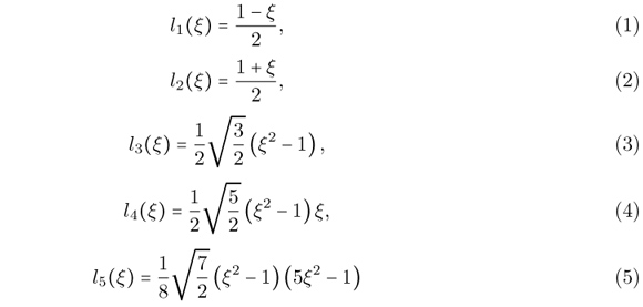
and

that are presented in Fig. 1. The mass and stiffness matrices can be obtained using the shape functions from Eqs. (1)-(6) by the standard procedure used for the FEM[7, 23, 42]. Here, the consistent mass matrix is used.

By assuming only the shape functions from Eq. (1) and Eq. (2) one obtains the lagrangian linear finite element[7, 23, 42]. However, the extra shape functions that allow higher order approximations are all zero at the nodes of the finite element. This ensures that the standard procedures used for the linear FEM still hold for the HFEM[36]. Imposition of boundary conditions and manipulation of nodal quantities remain the same as used for the FEM. Note that if more than one shape function is not zero in a given node of the finite element, special techniques must be used to impose the boundary conditions of the problem, such as the Lagrange Multiplier Method or some Penalty Method[12 ,13]. For this reason most hierarchical approaches introduce extra shape functions that are null at the nodes of the finite element.

The main characteristic of the HFEM is that when the order of the approximation is increased the shape functions already in use remain unchanged. The traditional FEM with shape functions given by Lagrange polynomials do not share this property, making the use of higher order approximations very difficult[36].

3 GENERALIZED FINITE ELEMENT METHOD

In the standard lagrangian FEM, the displacements inside a given finite element are approximated by[7, 8, 23, 42]

where u_i are nodal degrees of freedom, N_i are the polynomial shape functions, ξ is the local coordinate system of the element and n is the number of shape functions.

In the context of the GFEM, the approximation given by Eq. (7) can be enriched by considering an approximate solution given by

where ϕ_j are enrichment functions and c_j are the associated degrees of freedom. Here the enrichment functions ϕ_j are obtained using the PUFEM[31] as described by [3, 39].

In the PUFEM the shape functions are given by the multiplication of a Partition of Unity (PU) by basis functions appropriately chosen. The PU used here is the one defined by the shape functions obtained for the lagrangian linear finite element, since the sum of these functions results in one[8, 23]. This PU is as shown in Fig. 2 and respects the conditions described by [31].

In Fig. 2, the finite elements are tagged el. 1, el. 2, etc, while the functions that composed the PU are tagged η_Ω1, η_Ω2, etc. Each function η_Ωj is defined in a subdomain Ω_i that is defined by the union of two neighbor finite elements, except for Ω₁ and Ω₅. In the context of the PUFEM the subdomains Ω_i are called covers or patches. In general, each finite element is defined in the intersection between two patches. More details on the PUFEM can be found in[5, 31].

Inside a finite element with local coordinates ξ = [-1,1] the PU can be written as

and

that are shown in Fig. 3.

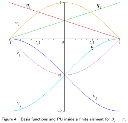
The basis functions used here are the ones proposed by [3]. Inside a finite element with local coordinates ξ = [-1,1] these functions can be written as

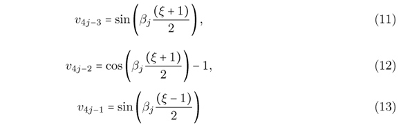
and

where β_j is a parameter that allows the modification of the shape functions. The basis functions and the PU for β_j = π are shown in Fig. 4.

The basis functions from Eqs. (11)-(14) were chosen as trigonometric functions since the analytical solution of most problems from dynamic analysis of bars are composed of trigonometric terms[15, 25, 32]. However, the basis functions from Eqs. (11)-(14) were carefully build as to result in shape functions that are zero at the nodes of the finite element, as discussed later.

In the context of modal analysis, an optimal value for β_j can be estimated in order to obtain best results for the approximation of a given fundamental vibration mode. An efficient iterative scheme for evaluating the optimal value for β_j was proposed by[,3] and leads to very accurate results.

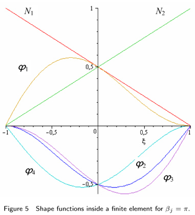
The shape functions for a finite element can be obtained by the multiplication of the PU by the basis functions, following the procedure described by[3]. The contribution from the patch to the left of the finite element is given by the multiplication of v_4j-3 and v_4j-2 by η₁. The contribution from the patch to the right is given by the multiplication of v_4j-1 and v_4j by η₂. The resulting PUFEM shape functions are:

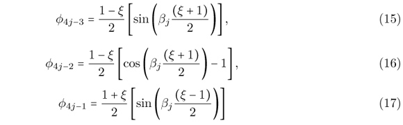
and

The nodal shape functions can be taken as η₁ and η₂ itself, that are the Lagrange linear polynomials. The approximation space is then given by

where V_GFEM is the approximation space of the GFEM used here, V_FEM is the approximation space from the FEM using linear finite elements and V_PUFEM is the approximation space obtained by the PUFEM and defined by the shape functions from Eqs. (15)-(18). The resulting shape functions for β_j = π are shown in Fig. 5. The mass and stiffness matrices can be obtained by the standard procedure used for the FEM [7, 23, 42]. Here, the consistent mass matrix is used.

By modifying the value of β_j one is able to adapt the shape functions for different cases[3]. Besides, several sets of enrichment function from Eqs. (15)-(18) can be considered by assuming different values of β_j. In order to build a finite element with 10 shape functions, for example, one can consider β₁ = π and β₂ = 2π and include 8 enrichment functions. Including more enrichment functions can be made without changing the enrichment functions already used and thus the GFEM proposed here is a hierarchical method. This simplifies computational implementation and allows the use of higher order approximations.

As can be seen from Fig. 5, the enrichment functions are zero at the nodes of the finite element. It can be demonstrated that this is true for any value of β_j. Consequently, the implementation of boundary conditions and manipulation of nodal quantities is the same as for the standard FEM and do not require special techniques. However, in order to ensure this property the basis functions were carefully designed. The use of other sets of trigonometric functions may not maintain this property.

Here, both the stiffness and mass matrices remain constant during the entire dynamic analysis. The same occurs for the shape functions. Consequently, the mass and stiffness matrices are evaluated only once, at the beginning of the dynamic analysis, and remain unchanged for the entire analysis. Once the stiffness and mass matrices are evaluated the dynamic analysis is made in the same way as occurs for the standard lagrangian FEM and the HFEM. In this work we have not checked the influence of time dependent shape functions, mass matrices and stiffness matrices. An approach where the shape functions are updated iteratively in order to comply with wave propagation angles was presented by[9], for a two dimensional problem.

The stiffness and mass matrices were obtained using analytical integration, by using software for symbolic manipulation. These matrices were obtained for a finite element with arbitrary values for the element length, elastic modulus, density, cross sectional area and the parameter β. The stiffness and mass matrices in closed form were then incorporated into the computational routine responsible for the dynamic analysis. It is important to point out that the analytical integration of the mass and stiffness matrices is not possible in most GFEM applications. In fact, numerical integration in the context of the GFEM is a delicate matter, since the shape functions may not be polynomials and then numerical integration may not be exact. A more detailed discussion on numerical integration for the GFEM is presented by [4]and [17].

The nodal degrees of freedom of the FEM, the HFEM and the GFEM (as presented here) are the same and are related to nodal displacements. These degrees of freedom are ruled by the linear lagrangian shape functions. However, the extra degrees of freedom of the HFEM and the GFEM (given by the Lobatto polynomials in the case of the HFEM and by the PUFEM shape functions in the case of the GFEM) have no direct physical meaning. These extra degrees of freedom affect the displacements inside the domain of the finite element, but are not particularly related to a single point of the domain, as occurs for the nodal degrees of freedom. For this reason, these extra degrees of freedom are also called field degrees of freedom.

Here, the field degrees of freedom are all zero at the nodes of the finite elements and thus nodal displacements can be obtained directly, by taking the value of the associated nodal degree of freedom. If one needs to evaluate displacements inside some finite element, then it is necessary to take into account the contribution of each shape function of the finite element. In this context, the way the degrees of freedom are defined for the HFEM and the GFEM do not affect the comparison of the results. In all three methods, nodal displacements can be read directly while displacements inside the finite elements can be evaluated by summing the contribution of all the shape functions, as occurs in the standard FEM.

4 TRUSS STRUCTURES

In order to obtain the equilibrium equations for a truss finite element, that can be oriented in an arbitrary direction in space, it is necessary to apply some coordinate transformation rule[33].

For a linear finite element of a planar truss the following coordinate transformation hold

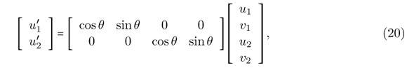
where u' are the nodal displacements in local coordinates, u and v are the horizontal and vertical nodal displacements in global coordinates and θ is the inclination of the bar.

The coordinate transformation for the HFEM and the GFEM follows the reasoning used by[41] for the Composite Element Method. Since the enrichment functions are zero at the nodes of the element, the coordinate transformation is given by

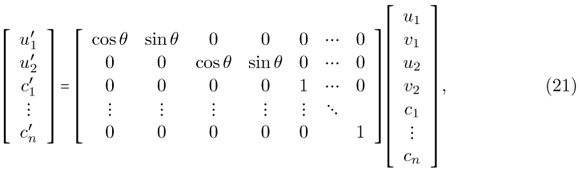
where c' are enrichment degrees of freedom in local coordinates and c are enrichment degrees of freedom in global coordinates. That is, the enrichment degrees of freedom in local coordinates are the same as the enrichment degrees of freedom in global coordinates.

5 ERROR EVALUATION

The error between the analytical solution u(x,t) and the approximate solution u_h(x,t) for a given position inside the bar x = x₀ in the time interval [t_i,t_f] can be defined as

In order to evaluate the error inside the entire bar one can integrate Eq. (22) along its length. However, this procedure is not used in this paper because of the computational difficulties involved in the evaluation of this integral.

Evaluating the error by using Eq. (22) may not be efficient in practice since the approximate solution is generally known only at discrete time steps. However, an approximation for Eq. (22) can be written as

where n_t is the number of time steps used, Δt is the time step used to obtain the approximate solution, u⁽ⁱ⁾ is the analytical solution at time step (i) and u_h⁽ⁱ⁾ is the approximate solution at time step (i).

Error evaluation according to Eq.(23) is illustrated in Fig. 6. The integral from Eq. (22) in a given time interval is approximated by the product between Δt and Δu⁽ⁱ⁾. Equation (23) can be evaluated efficiently since it only deals with discrete values in time. More details on error evaluation for the time response are presented by[39].

6 NUMERICAL RESULTS

6.1 Bar subject to initial displacements

The first example is that of a bar fixed at both ends and subject to initial displacements as shown in Fig. 7. The properties of the material were chosen to give the wave velocity equal to c = = 1m/s and the bar length is equal to 1m. The initial displacement field is zero at both ends, has a maximum value u_max equal to 0.25m at the middle of the bar and has a triangular shape. This initial displacement can be obtained by applying a unitary load at the middle of the bar. Finally, there is no force acting on the bar and the initial velocities are null.

This problem can be stated as[38]

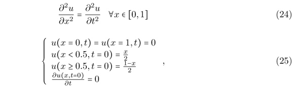
that is a wave propagation problem with wave velocity c = 1m/s. The analytical solution can be found by separation of variables and by representing the initial conditions by a Fourier series as described by [25].

This example is first studied using Modal Superposition for a time interval of 20s and using 11 degrees of freedom. The resulting equations from Modal Superposition are solved using the Newmark method (with α = 0.5 and δ = 0.25) for a time step equal to 2.5x10^-3s. For the FEM the mesh is composed of 10 linear finite elements. For the HFEM the mesh is composed of two finite elements of order 5, by assuming 6 polynomial shape functions. For the GFEM the mesh is composed of two finite elements with 4 enrichment functions as given by Eqs. (15)-(18), by assuming β₁ = 3π/2. The analytical and the approximate solutions at x = 0.5m are presented in Fig. 8, considering 5 modes in Modal Superposition.

The errors for different numbers of modes included in the Modal Superposition analysis are presented in Table 1. The errors obtained by considering only the first mode are presented in the first column, the errors obtained by considering the first two modes are presented in the second columns and so on. The errors from Table 1 are also presented in Fig. 9.

It can be seen that the best results were not obtained by considering every fundamental vibration mode of the structure. This is a general trend when dealing with Modal Superposition because the higher vibrations modes of the structure may be poorly approximated by the FEM[13]. Consequently, including the higher vibrations modes in Modal Superposition may reduce the accuracy of the approximate solution.

From Table 1 and Fig. 9 it can be seen that the best results were obtained with the GFEM when considering 5 or 6 modes. The best results for the HFEM were obtained when 3 or 4 modes were considered. The results obtained with the FEM are very poor in comparison to the ones obtained with both the HFEM and the GFEM. This behavior is confirmed by the displacements presented in Fig. 8.

From Fig. 9 another interesting conclusion can be drawn. The inclusion of the fifth mode improved the solution given by the GFEM, but worsened the solution given by the HFEM. This seems to indicate that the higher modes are better approximate by the GFEM in this case.

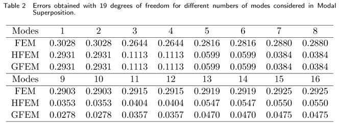
The same problem was also solved using 19 degrees of freedom. The mesh used for the FEM is composed of 18 linear finite elements. The mesh used for the HFEM is composed of 2 finite elements of order 9, by assuming 10 polynomial shape functions. For the GFEM the mesh is composed of two finite elements with 8 enrichment functions as given by Eqs. (15)-(18), by assuming β₁ = 3π/2 and β₂ = 3π. The errors for these cases are presented in Table 2 and Fig. 10.

As expected the errors were reduced when more degrees of freedom were used. The best results for 19 degrees of freedom were obtained with the GFEM when considering 9 or 10 modes. However, the results obtained with the GFEM and the HFEM are now very similar. The results given by the FEM are very poor if compared to the two other methods.

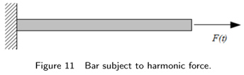
6.2 Bar subject to harmonic force

The second example is that of a bar fixed at one end and subject to a harmonic force at the other end, as shown in Fig. 11. The properties of the material were chosen to give the wave velocity equal to c = = 1m/s and the bar length is equal to 1m. The initial displacements and velocities are zero.

For a force given by

the problem can be stated as[38]

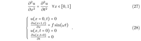
The analytical solution of this problem is more difficult to obtain than the previous one since the boundary condition representing the harmonic force is not homogeneous. The problem can be solved using techniques described by [32] and is reproduced here since it was not found elsewhere. Considering c as the wave velocity, the displacements are given by

where

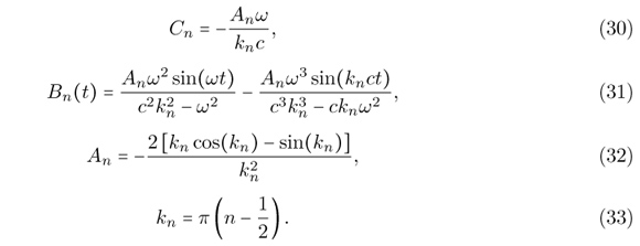
This problem is solved numerically for ω = 20rad/s and f = 1N/m². The analysis is made using the Modal Superposition Method for a time interval of 20s and the resulting equations are solved using the Newmark method (with α = 0.5 and δ = 0.25) for a time step equal to 1.25x10^-3s.

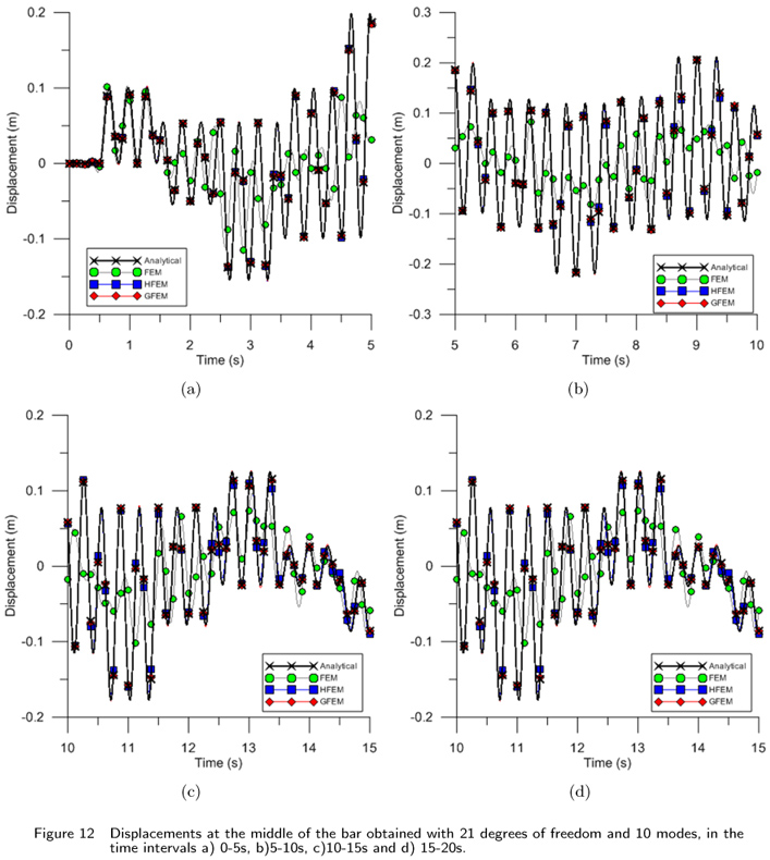
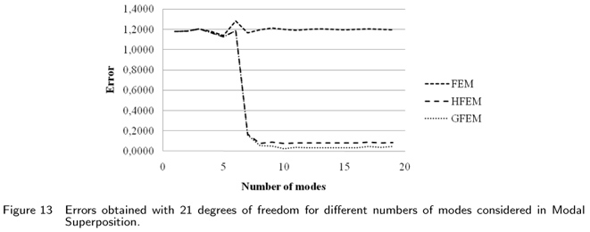
The first comparison is made using 21 degrees of freedom. The mesh of the FEM is composed of 20 linear finite elements, while the mesh of the HFEM is composed of 4 finite elements of order 5. The mesh of the GFEM is composed of 4 finite elements with 4 enrichment functions considering β₁ = 3π/2. The analytical and the approximate solutions at x = 0.5m considering 10 modes in Modal Superposition are presented in Fig. 12.

The errors for this example are presented in Table 3 and Fig. 13. The best result was obtained with the GFEM when considering 10 modes and corresponds to an error of 0.0258. The best result obtained with the HFEM was also obtained with 10 modes, but the error in this case is 0.0722. The results given by the FEM are much less accurate than the results obtained with the other two methods, as can be seen from Fig. 12.

A closer inspection of Fig. 12 reveals that the displacements obtained with the HFEM and the GFEM in the time interval 0-10s are both very similar to the analytical solution. However, the results given by the HFEM for the time interval 10s-20s present some deviation from the analytical solution, mainly for peak displacements. The solution given by the GFEM, instead, is very close to the analytical solution even in these cases.

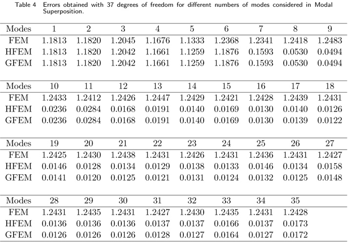
This example is also solved using 37 degrees of freedom. The FEM mesh is composed by 36 linear finite elements, the HFEM mesh is composed of 4 elements of order 9, and the GFEM mesh is composed of two finite elements with 8 enrichment functions, by assuming β₁ = 3π/2 and β₂ = 3π. The errors for these cases are presented in Table 4 and Fig. 14. The displacements obtained using 37 degrees of freedom and 20 modes are presented in Fig. 15.

From both Table 4 and Fig. 14 it can be seen that the results given by the HFEM and the GFEM are very similar. The best results for both methods were obtained when considering 20 modes in the Modal Superposition analysis. The results given by the FEM are much less accurate than the ones obtained with the other two methods.

The comparison between the errors obtained with the linear FEM from Table 3 and Table 4 indicate that the errors remained almost the same when more degrees of freedom were used. Even if this result seems contradictory, since one expects the errors to be reduced when the approximation is improved, the reason for this occurrence can be found by comparing the displacements from Fig. 12 and Fig. 15. The overall approximation given by the FEM when considering 37 degrees of freedom is better than when considering 21 degrees of freedom, except at the time interval 12s-18s. From Fig. 15 it can be seen that the approximation given by the FEM with 37 degrees of freedom is very poor in the time interval 12s-18s, even worse than the ones obtained with 21 degrees of freedom. This increases the error in the total time interval 0s-20s to the same level as those observed when using 21 degrees of freedom.

When Modal Superposition is used, the analyst is able to improve the approximate solution by removing the poorly approximated higher modes from the analysis[7], as can be observed in the results of the last two examples. However, in the case that direct integration methods are used one is not able to choose which modes will be considered. According to[7], direct integration methods are expected to give the same results that would be obtained with Modal Superposition by including all fundamental modes in the analysis. The error imbued by the higher modes when using direct integration methods must then be reduced by using appropriate time steps or some kind of numerical damping[7, 23].

In this context, the numerical damping that occurs when some time integration schemes are used (note that not all time integration schemes give numerical damping) can be beneficial, since the influence of the higher vibration modes (that are poorly approximated) can be damped out. The Houbolt Method naturally includes some kind of numerical damping, but the analyst is not able to control the magnitude of this damping[7, 23]. Some time integration schemes that include numerical damping and allow the analyst to control the magnitude of this damping in some way are the α-HHT method[21, 23] and the generalized-α method[24]. Here we use the Newmark method (with α = 0.5 and δ = 0.25), that according to[7] do not cause numerical damping, since we are interested in evaluating the ability of the GFEM and the HFEM to approximate the higher vibration modes of the structures. The comparison of the FEM, the HFEM and the GFEM together with other time integration schemes should be subject of further investigation.

The results presented for the previous two examples indicate that the GFEM was able to obtain better approximations than the HFEM and the FEM when all modes were included in Modal Superposition, possibly because the higher modes have been better approximated by the GFEM. This behavior plays an important role when direct integration methods are used, since in this case the analyst is not able to exclude the influence of higher vibration modes from the analysis.

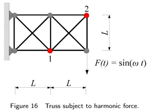
6.3 Truss subject to harmonic force

The third example is that of the truss from Fig. 16, that is subjected to a harmonic force and null initial displacements and velocities. In this case it is not possible to increase the number of degrees of freedom when using the FEM with linear elements, since each bar cannot be divided in two finite elements without making the structure unstable. When using the GFEM and the HFEM, instead, it is possible to increase the number of degrees of freedom by increasing the number of shape functions used.

All bars have E = 210GPa, A = 0.005m², ρ = 8000kg/m³ and the truss has L = 3m. The example is solved assuming an applied force with magnitude f = 1000N and three different frequencies: ω = 5000rad/s, ω = 7500rad/s and ω = 10000rad/s. No analytical solution is known for this problem and it is solved only by the approximate methods. Thus no error evaluation is performed and the comparison between the results is only qualitative.

The problem is solved using the Newmark method (with α = 0.5 and δ = 0.25) with a time step equal to 1.0x10^-5s. Four different meshes are considered: a) FEM with linear elements, b) HFEM with 6 shape functions per bar, c) GFEM with 6 shape functions per bar, d) HFEM with 10 shape functions per bar and e) GFEM with 10 shape functions per bar. All bars of the structure are considered as a single finite element. In the case of the GFEM the enrichment functions are obtained with β₁ = 3π/2 when 6 shape functions are considered and with β₁ = 3π/2 and β₂ = 3π when 10 shape functions are considered.

The vertical displacements at node 1 from Fig. 16 for ω = 5000rad/s are presented in Fig. 17. In this case it can be seen that both the HFEM and the GFEM obtained the same results when using 6 and 10 shape functions per bar. The results obtained with the FEM with linear elements, instead, is different from the ones obtained with the HFEM and the GFEM.

The vertical displacements at node 1 for ω = 7500rad/s are presented in Fig. 18. The HFEM and the GFEM converged to the same results when 10 shape functions per bar were used and thus only the results for the HFEM with 10 shape functions are presented. Taking as reference the solutions obtained with 10 shape functions per bar, a close inspection of Fig. 18 seems to indicate that the GFEM with 6 shape functions obtained more accurate results than the HFEM with 6 shape functions. The displacements obtained with the FEM are very different from the ones obtained with the other two methods.

The vertical displacements at node 1 for ω = 10000rad/s are presented in Fig. 19. The displacements obtained with the HFEM and GFEM using 10 shape functions per bar converged to the same results again. For this reason only the results given by the HFEM using 10 shape functions are presented. Taking as reference the solutions obtained with 10 shape functions per bar, Fig. 19 indicates that the GFEM with 6 shape functions obtained more accurate results than the HFEM with 6 shape functions per bar. Besides, the difference between the solutions obtained with 6 shapes functions per bar is more noticeable in this case than for ω = 7500rad/s.

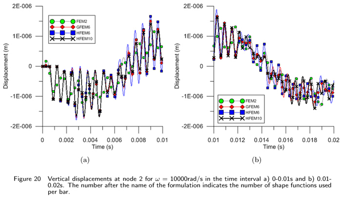
The vertical displacements at node 2 for ω = 10000rad/s are presented in Fig. 20. The same conclusions drawn for the displacements at node 1 hold in this case. It seems that the GFEM with 6 shape functions obtained more accurate results than the HFEM with 6 shape function, taking as reference the solutions obtained with 10 shape functions per bar.

The comparisons made for the three different frequencies indicate that the GFEM is able to obtain better results than the HFEM for higher frequencies, as observed in the previous examples and by[3].

6.4 Bar subject to impact load

The fourth example is that of a bar subject to an impact load. The bar is initially at rest and is subject to the same boundary conditions as shown in Fig. 11. The properties of the bar are now E = 210GPa, A = 0.001m², ρ = 8000kg/m³ and L = 1m.

The time dependent load is given by

where f is the force magnitude and t_f is the time when the force stops. This applied force is as shown in Fig. 21 and is used to model the impact load.

Here we assume f = 1000N and t_f = 0.001s. Note that very different time responses are obtained when the value of t_f is changed. The problem is solved using the Newmark method (with α = 0.5 and δ = 0.25) with a time step equal to 2.5x10^-7s.

The displacements at the middle of the bar are presented in Fig. 22. The analysis was made using 11 degrees of freedom. In the case of the linear FEM, this mesh is given by dividing the domain into 10 finite elements. In the case of the GFEM and the HFEM the mesh is obtained by dividing the domain into 2 finite elements and assuming 6 shape functions per finite element. For the GFEM β is taken equal to 3π/2. The reference solution is taken as the solution given by the HFEM when using 4 finite elements with 10 shape functions. This results in 37 degrees of freedom.

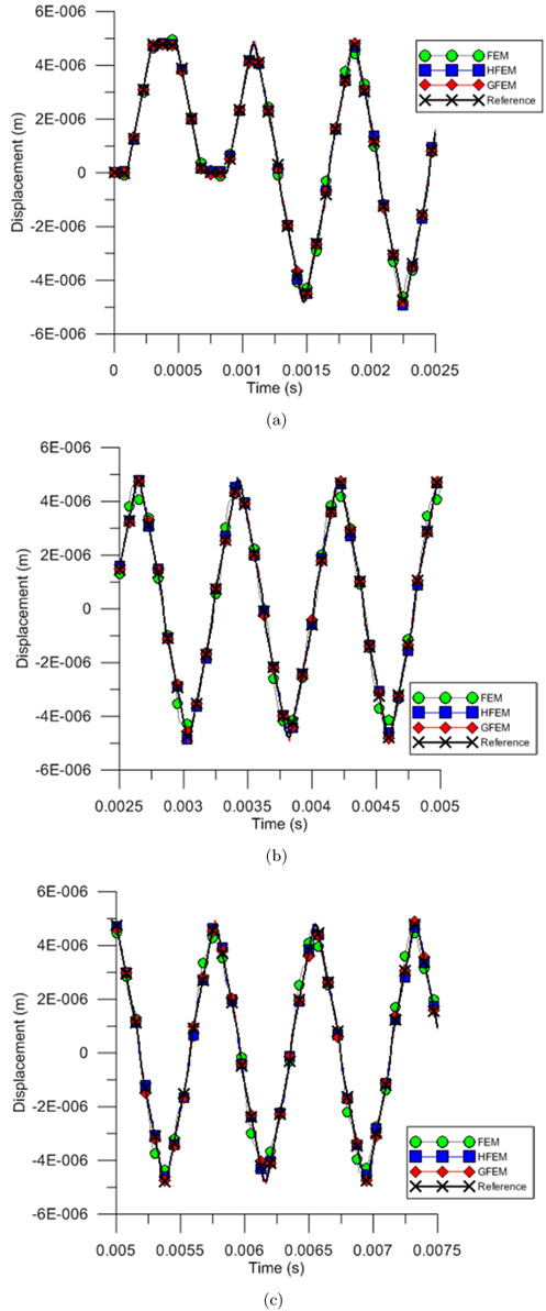
From the results presented in Fig. 22 it can be seen that the results given by the HFEM and the GFEM are very close to the reference solution. The results given by the linear FEM, are also able to represent the main trend of the vibration, but are not as close to the reference solution. This is especially true for peak displacements and larger time intervals, as can be seen in Fig. 22d. The lost of accuracy for larger time intervals appears to be reduced when the HFEM and the GFEM are used.

6.5 Truss subject to impact load

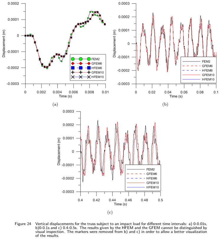
The last example is that of the truss from Fig. 23 that is subject to an impact load. The truss nodes are equally spaced and dx = dy = 2m. The material has properties E = 210GP and ρ = 8000kg/m³ while all bars have a cross sectional area equal to A = 0.001m². There is an applied force at the central node of the lower chord. This load is as defined in Eq. and Fig. 21, with magnitude f = 10kN and t_f = 0.001s, and represents an impact load.

The problem is solved using the Newmark method (with α = 0.5 and δ = 0.25) with a time step equal to 1.0x10^-5s. Each bar is modeled as a single finite element. In the case of the HFEM and the GFEM the analysis is made using 6 and 10 shape functions per finite element. For the GFEM we assume β = 3π/2 and β = 3π. For the linear FEM only 2 shape functions are used. Note that the bars cannot be divided in two without creating an unstable structure and consequently it is not possible to refine the mesh when using the linear FEM. The vertical displacements at the node put in evidence in Fig. 23 are presented in Fig. 24, for three different time intervals.

The results given by the HFEM and the GFEM with 6 and 10 shape functions cannot be distinguished by visual inspection. From the time interval 0-0.01s, presented in Fig. 24a, we note that the displacement wave takes some time in order to arrive at the node monitored. It is also possible to see that the results given by the HFEM and the GFEM are very similar, while the displacements given by the linear FEM are not coincident with the displacements obtained with the other methods.

From Fig. 24b and Fig. 24c we note that the linear FEM is able to represent the main trend of the displacements, but that accuracy is lost for larger time intervals. This lost of accuracy for larger time intervals appears to be reduced when the HFEM and the GFEM are used. This kind of behavior of the linear FEM can lead to difficulties for obtaining very accurate results with the linear FEM, since the mesh cannot be refined just by dividing the finite elements in two.

7 CONCLUSIONS

This paper presented a GFEM formulation for the dynamic analysis of bars and trusses. The time integration procedure was made using Modal Superposition and the Newmark method. Numerical errors can result both from the time integration procedure and from the finite element approximation. Errors from the numerical integration procedure can be reduced by decreasing the time step used or by changing the number of modes considered for Modal Superposition, while errors from the finite element method can be reduced by using a more accurate approximation.

The GFEM allows one to use an enriched approximation for the displacements that is easy to obtain and does not affect nodal quantities. This approximation leads to better results than standard linear FEM. For the examples studied here, the GFEM also presented better results than the HFEM. Besides, this GFEM formulation presented here is a hierarchical one (as is the case of HFEM), since the approximation can be enriched without changing the shape functions used in lower order elements. Finally, the enrichment shape functions proposed do not affect the nodal degrees of freedom and thus standard procedures used for the linear FEM still hold.

The results presented here indicate a strong potential of the GFEM for problems from structural dynamics. The extension of the approach proposed in this paper to beams and two dimensional problems will be subject of future works.

Received 09 Apr 2012

In revised form 08 May 2012

• [1] Y. Abdelaziz and A. Hamouine. A survey of the extended finite element. Computers & Structures, 86:11411151, 2008.
• [2] M.H. Aliabadi. The boundary element method: applications in solids and structures John Wiley & Sons, Chichester, 2002.
• [3] M. Arndt, R.D. Machado, and A. Scremin. An adaptive generalized finite element method applied to free vibration analysis of straight bars and trusses. Journal of Sound and Vibration, 329:659672, 2010.
• [4] Babuska, U. Banerjee, and J.E. Osborn. Generalized finite element methods: main ideas, results, and perspective. Technical report, TICAM, University of Texas at Austin.
• [5] Babuska and J.M. Melenk. The partition of unity method. International Journal for Numerical Methods in Engineering, 40(4):727758, 1997.
• [6] N.S. Bardell. Free vibration analysis of a flat plate using the hierarchical finite element method. Journal of Sound and Vibration, 151(2):263289, 1991.
• [7] K.J. Bathe. Finite element procedures Prentice Hall, Upper Saddle River, 1996.
• [8] E.B. Becker, G.F. Carey, and J.T. Oden. Finite elements: an introduction. Prentice-Hall, Englewood Cliffs, 1981.
• [9] E. De Bel, P. Villon, and P. Bouillard. Forced vibrations in the medium frequency range solved by a partition of unity method with local information. International Journal for Numerical Methods in Engineering, 62:11051126, 2005.
• [10] O. Beslin and J. Nicolas. A hierarchical functions set for predicting very high order plate bending modes with any boundary conditions. Journal of Sound and Vibration, 202(5):633655, 1997.
• [11] C.A. Brebbia and D. Nardini. Dynamic analysis in solid mechanics by an alternative boundary element procedure. Soil Dynamics and Earthquake Engineering, 2(4):228233, 1983.
• [12] F. Brezzi and M. Fortin. Mixed and hybrid finite element methods. Springer-Verlag, New York, 1991.
• [13] G.F. Carey and J.T. Oden. Finite elements: a second course Prentice-Hall, Englewood Cliffs, 1983.
• [14] J.A.M. Carrer and W.J. Mansur. Stress and velocity in 2d transient elastodynamic analysis by the boundary element method. Engineering Analysis with Boundary Elements, 23:233245, 1999.
• [15] A.K. Chopra. Dynamics of structures: theory and applications to earthquake engineering. Prentice Hall, Englewood Cliffs, 1995.
• [16] C. Daux, N. Moes, J. Dolbow, N. Sukumar, and T. Belytschko. Arbitrary branched and intersecting cracks with extended finite element method. International Journal for Numerical Methods in Engineering, 48:17411760, 2000.
• [17] C.A. Duarte and D.J. Kim. Analysis and applications of a generalized finite element method with global-local enrichment functions. Computer Methods in Applied Mechanics and Engineering, 197:487504, 2007.
• [18] R.C. Engels. Finite element modeling of dynamic behavior of some basic structural members. Journal of Vibration and Acoustics, 114:39, 1992.
• [19] N. Ganesan and R.C. Engels. Hierarchical bernoulli-euller beam finite elements. Computers & Structures, 43(2):297304, 1992.
• [20] L. Hazard and P. Bouillard. Structural dynamics of viscoelastic sandwich plates by the partition of unity finite element method. Computer Methods in Applied Mechanics and Engineering, 196:41014116, 2007.
• [21] H.M. Hilber, T.J.R. Hughes, and R.L. Taylor. Improved numerical dissipation for time integration algorithms in structural dynamics. Earthquake Engineering and Structural Dynamics, 5:283292, 1977.
• [22] A. Houmat. An alternative hierarchical finite element formulation applied to plate vibrations. Journal of Sound and Vibration, 206(2):201215, 1997.
• [23] T.J.R. Hughes. The finite element method: linear static and dynamic finite element analysis Prentice Hall, Englewood Cliffs, 1987.
• [24] J.Chung and G.H. Hulbert. A time integration algorithm for structural dynamics with improved numerical dissipation: the generalized- method. Journal of Applied Mechanics, 60:371375, 1993.
• [25] E. Kreyszig. Advanced engineering mathematics John Wiley & Sons, Singapore, 2006.
• [26] A.Y.T. Leung and J.K.W. Chan. Fourier p-element for the analysis of beams and plates. Journal of Sound and Vibration, 212(1):179185, 1998.
• [27] R.J. LeVeque. Finite difference methods for ordinary and partial differential equations: steady-state and time-dependent problems SIAM, Philadelphia, 2007.
• [28] E. Levy and M. Eisenberger. Dynamic analysis of trusses including the effect of local modes. Structural Engineering and Mechanics, 7(1):8194, 1999.
• [29] G.R. Liu. Mesh free methods: moving beyond the finite element method CRC Press, Boca Ratton, 2003.
• [30] W.K. Liu, S. Jun, S. Li, J. Adee, and T. Belytschko. Reproducing kernel particle methods for structural dynamics. International Journal for Numerical Methods in Engineering, 38(10):16551679, 1995.
• [31] J.M. Melenk and I. Babuska. The partition of unity finite element method: Basic theory and applications. Computer Methods in Applied Mechanics and Engineering, 139(1-4):289314, 1996.
• [32] Y. Pinchover and J. Rubinstein. An Introduction to partial differential equations Cambridge University Press, Cambridge, 2005.
• [33] S.S. Rao. The finite element method in engineering Elsevier, Amsterdam, 2005.
• [34] P. Ribeiro. Hierarchical finite element analyses of geometrically non-linear vibration of beams and plane frames. Journal of Sound and Vibration, 246(2):225244, 2001.
• [35] P. Rozycki, N. Moes, E. Bechet, and C. Dubois. X-fem explicit dynamics for constant strain elements to alleviate mesh constraints on internal or external boundaries. Computer Methods in Applied Mechanics and Engineering, 197:349363, 2008.
• [36] P. Solín, K. Segeth, and I. Dolezel. Higher-order finite element methods Chapman & Hall/CRC, Boca Raton, 2004.
• [37] Strouboulis, K. Copps, and I. Babuska. The generalized finite element method. Computer Methods in Applied Mechanics and Engineering, 190:40814193, 2001.
• [38] S. Timoshenko and J.N. Goodier. Theory of elasticity McGraw-Hill, New York, 1951.
• [39] A.J. Torii and R.D. Machado. Transient dynamic structural analysis of bars and trusses using the generalized finite element method. In In: E. Dvorkin, M Goldschmit and M. Storti (Eds.). Mecánica Computacional. Buenos Aires: Asociacion Argentina de Mecánica Computacional, volume 24, pages 18611877, 2010.
• [40] P. Zeng. Composite element method for vibration analysis of structure, part ii: C1 element(beam). Journal of Sound and Vibration, 218(4):659696, 1998.
• [41] P. Zeng. Composite element method for vibration analysis of structures, part i: principle and c0 element(bar). Journal of Sound and Vibration, 218(4):619658, 1998.
• [42] O.C. Zienkiewicz and R.L. Taylor. The finite element method, Volume 1: The Basis Butterworth-Heinemann, Oxford, 2000.

Publication Dates

• Publication in this collection
  17 Jan 2013
• Date of issue
  June 2012

History

• Received
  09 Apr 2012
• Reviewed
  08 May 2012