A Model Analysis for the Design and Deployment of an Eulerian Sediment Trap Mooring Array in a Western Boundary Upwelling System from Southeast Brazil

Abstracts

This work addresses the design and configuration of a Eulerian sediment trap mooring array, which was deployed at the shelf edge (z_m ≈ 140 m) 80 km off Cabo Frio, SE- Brazil (23° S). The site was subject to interplay between the Tropical Waters (TW) of the Brazil Current (BC), intrusions from the South Atlantic Central Waters (SACW), which are the source of upwelling in the region, and other oceanographic processes. Detailed computations were used to optimize the total weight, buoyancy balance, and maximum acceptable tilt to avoid hydrodynamic bias in the trapping efficiency and array adaptation to the local oceanographic conditions with the assistance of Matlab and Muringa programs and Modular Ocean Model 4.0 (MOM; i.e., to assert the vertical distribution of the meridional current component). The velocity range of the current component was determined by short term measurements to be between 0.1 and 0.5 m/s. Projections led to a resulting minimum anchor weight of 456 kg. The necessary line tension was ascertained by using the appropriate distribution of a series of buoys along the array, which finally attained a high vertical load of 350 kg because of the attached oceanographic equipment. Additional flotation devices resulted in a stable mooring array as reflected by their low calculated tilt (2.6° ± 0.6°). A low drag of 16 N was computed for the maximum surface current velocity of 0.5 m/s. The Reynolds number values ranged from 4 × 10⁴ to 2 × 10⁵ and a cone-trap aspect ratio of 1.75 was used to assess the trap sampling efficiency upon exposure to different current velocities.

design; mooring array; sediment traps; trap efficiency; Cabo Frio upwelling; SE-Brazil

Esta contribuição dirigiu-se aos procedimentos adotados para o desenho e configuração de uma linha de fundeio eulariana com armadilhas de sedimentação, a qual foi instalada na borda da plataforma (z_m ≈ 140 m) a 80 km de Cabo Frio, SE-Brasil (23°S). O local foi sujeito à dinâmica entre a Água Tropical (AT) da Corrente do Brasil (BC), intrusões da Água Central do Atlântico Sul (ACAS), as quais são a fonte da ressurgência na região, e outros processos oceanográficos. Computações detalhadas foram utilizadas para aperfeiçoar o peso total, o balanço da flutuação e a inclinação máxima aceitável para evitar um erro hidrodinâmico na eficiência de captura e adaptação da linha do fundeio às condições oceanográficas locais, assistidas pelos programas Matlab e Muringa, e o Modelo Oceânico Modular 4,0 (MOM; para inferir a distribuição vertical do componente meridional da corrente). A faixa de velocidade da componente da corrente entre 0,1 e 0,5 m/s foi determinada através de medições curtas. As projeções levaram a um peso mínimo da âncora resultando em 456 kg. A tensão da linha requerida foi verificada utilizando a distribuição apropriada de uma série de bóias ao longo do fundeio, a qual finalmente alcançou uma alta carga vertical de 350 kg devido aos equipamentos oceanográficos incluídos. Aparelhos adicionais de flutuação resultaram em uma linha de fundeio estável como refletido pela baixa inclinação calculada (2,6° ± 0,6°). O baixo arrasto de 16 N foi computado para a corrente superficial máxima de 0,5 m/s. Os valores do número de Reynolds variaram de 4 × 10⁴ para 2 × 10⁵ e a razão da feição da armadilha cônica de 1,75 foi utilizada para avaliar a eficiência da amostragem da armadilha após exposição a diferentes velocidades de correntes.

desenho; linha de fundeio; armadilhas de sedimentação; eficiência de captura; ressurgência de Cabo Frio; SE-Brasil

INTRODUCTION

Time-series sediment traps (TS-traps) have been used to measure inorganic and organic particle fluxes and associated elements, including carbon, from the surface to the bottom of the oceans (Suess 1980, Honjo et al. 1992). The particle flux can be determined at any site using a receptacle (sediment trap) placed in the water column to intercept the settling particles. The flux is then calculated from the mass of collected particles divided by the aperture (collecting area) of the receptacle and the integrated time of its exposure in the water column. A number of devices and oceanographic tools have been developed in parallel, such as conical and cylindrical traps attached to Eulerian mooring arrays for longer term studies and free-floating neutrally buoyant (Lagrangian) sediment traps for short term studies within a given water mass (see review by Asper 1996).

With the Eulerian approach, the sediment traps are positioned at different water depths and fixed along a mooring line to which other oceanographic sensors are attached, to measure a number of prime variables, such as current velocity and direction, water temperature, salinity, turbidity and chlorophyll, which are needed for interpretating particle fluxes. The mooring line of the array is tethered to the bottom with a weight and an anchor and has subsurface floats distributed in accordance to the location and weight of the equipments along the line. Acoustic releasers are used to detach the array from the weight, enabling its uplift and recovery at the ocean surface (Gardner 1980).

The deployment of Eulerian sediment trap arrays may involve a number of caveats if the necessary attention is not given to trap design and configuration. The following two main features, among many other details, must be taken into account: 1) the “hydrodynamic bias” generated by hydrodynamic effects on the sediment trap opening must be minimized. Excessive shear and turbulence may impede the settling particles from entering the trap and enhance “selective particle sedimentation” (Gardner 1985, Asper 1988). This result is generally achieved by covering the opening with a baffle and positioning the traps in deeper waters with reduced flow; and 2) the mooring array must be designed in accordance with the specific oceanographic conditions of the study site.

The degree of lateral advection and variability in velocity and direction, which also varies vertically along the mooring array, must be accommodated. The weight and drag coefficient of the array are also affected by the form and vertical distribution of the sediment traps and other attached equipment. All of these features should be computed together to ascertain the vertical stability with minimum tilting by the entire array to maximize particle trapping efficiency (Gardner 1985). The stability of the array and acceptable degree of inclination (tilt) to its main axis is given by the calculation of an ideal ratio between the down lift and uplift potential (i.e., the buoyancy balance) as a function of lateral advection (Gardner 1980, 1985, Butman et al. 1986, Honjo et al. 1992, Tsinker 1994, Asper 1996, Bale 1998).

Since the 1970's, significant efforts have been devoted to the design and configuration of sediment trap mooring arrays for the open ocean, including large scale intercalibration experiments of sediment traps in situand the in vitro flume behavior (Honjo et al. 1992, Buesseler et al. 2007). However, special attention is needed when sediment trap mooring arrays are deployed in the shallower continental shelf waters in comparison to those of the open ocean, because of the dynamic interactions between multi-layered coastal and oceanic currents, shorter temporal and vertical changes in current velocities and directions, across-shelf transport mechanisms generated by tidal pumping, internal wave and wind-induced vertical mixing of the water column, and resuspension processes of bottom materials and in upwelling regions as governed by a marked variability in the proliferation and pulsation of the water mass between the shelf edge and inner shelf (Castro and Miranda 1998, Chavez and Toggweiler 1995, Honjo 1996, Pilskain et al. 1996, Fischer et al. 2009).

This study demonstrates the design and configuration of a sediment trap array prior to its deployment at the shelf edge (z_m ≈ 140 m) 80 km offshore of Cabo Frio, state of Rio de Janeiro, SE Brazil. The study included the use of Matlab and Muringa programs, as well as the Modular Ocean Model (MOM 4.0), to obtain information on the vertical distribution of the meridional current component. The study design considered the hydrodynamic conditions in order to correct and/or reduce mechanical and hydrodynamic biases caused by in situ oceanographic fluid motion conditions and the determination of sediment trap efficiencies based on the fluid dynamic principles of a conical TS trap with current modeled measurements.

This project corresponds to a series of studies within the scope of the “Upwelling Project” (“Projeto Ressurgência” in Portuguese) as carried out by the Brazilian Oil Company PETROBRAS/CENPES at the boundary between the Campos and Santos Basins, which is on the SE Brazil shelf. The overall aim of the project is to assess regional particle fluxes from the water column, particle deposition, burial and paleo-reconstruction processes of the shelf and/or their export to the ocean in relation to oceanographic processes. Following Albuquerque et al. in press, this issue, presents estimates of particle fluxes and their geochemical composition comprising several trap exposure periods between the late spring of 2010 and summer 2012, whereas Belem et al. (2013) described the oceanographic results from late spring 2010 and autumn 2011. Further information on the project and the Geochemical Network maintained by CENPES/PETROBRAS can be found at www.loop-uff.org.

Study Areas and Oceanographic Setting

The coastal western boundary upwelling system off Cabo Frio (23° S) in the western South Atlantic Ocean is one of the few western boundaries with upwelling systems in the world (e.g. Florida Current: Smith 1983; east Australian current: Roughan and Middleton 2002). This intermittent upwelling is predominantly related to the winds from the northeast (Castro and Miranda 1998), which are generated by the anticyclone of the South Atlantic during spring and summer, and it is interrupted by the passage of southwest frontal systems (Moreira and Rodrigues 1966, Carbonel 2003). Other mechanisms that can enhance the upwelling have been described, such as the interaction between flow and shelf topography (Rodrigues and Lorenzzetti 2001), the passage of meanders and eddies to produce instability in the Brazil Current (Campos et al. 2000) and vertical transport driven by wind stress curl (Castelao and Barth 2006, Castelao 2012). Multiple upwelling mechanisms can be important, as also reported for other western boundaries (Roughan and Middleton 2002). The upwelling water mass in Cabo Frio is characterized by the colder (T< 20°C), fresher (S< 36.4) South Atlantic Central Waters (SACW) underlying the warmer (T> 20°C), salty (S> 36.4) Tropical Water (TW) (Castro and Miranda 1998).

Environmental issues and the structure and function of the coastal shelf oceanic realms in the Campos and Santos Basins, off the state of Rio de Janeiro have raised concerns with PETROBRAS and the regional communities themselves, since the systems are the most productive oil and gas basins in Brazil. More than 70% of the petroleum prospected in the country comes from platforms located in this area.

MATERIALS AND METHODS

Location of the Mooring

The original intention was to deploy a subsurface mooring of 102 m length at the outer continental shelf at a depth of 120 m. However, the mooring was eventually tethered to the bottom at 145 m depth, ∼80 km offshore from the Cabo Frio coast, in the state of Rio de Janeiro (23°36′ S - 41°34′ W; Figure 1) during the deployment.

Figure 1 -
Study area offshore from Cabo Frio on the southeastern Brazilian Shelf. The mooring site is marked with a black triangle.

Mooring Layout

Mooring buoyancy was assured by a steel (37″) buoy and seven three-glass (12″) flotation modules (McLane Inc.) attached along the mooring line with center rods (Figure 2). The mooring line was made of 3.16″ torque balance jacketed (3 × 19) wire-rope (Mooring System, Inc.) to resist rotation, and was intercalated with a twist of galvanized steel chain (3.8″). A wire-rope was the principal tension element for raising and lowering the mooring components (Chaplin 1999). All of the shackles, pear links and swivels were made of galvanized steel. To assure retrieval in case the mooring line drifted or snapped, a Subsurface Mooring Monitoring Beacon (SMM) was switched on as the line approached the surface. An alarm state was set upon reception of the signal by an orbital satellite, which relayed the position to the CLS (Collect Localization Satellites) of the Argos monitoring service. A turbidity /fluorometer sensor (FLNTUSB) was placed at a depth of 25 m.

Figure 2 -
The Cabo Frio subsurface mooring array layout intended to deploy at a depth of 120 m.

Two programmable traps with conical funnels (Parflux Mark 8-13; McLane Research Laboratories, Inc. Falmouth, MA) designed primarily for oceanic deployments were placed in sequence along the mooring line. The traps had one large (660 mm diameter) conical baffle collector that fed the settling particles into 13 separate sampling cups held in a 14-port carousel. The trap at the top (25 m) of the mooring line was placed above the pycnocline to capture the material from the euphotic zone, whereas the lowest trap (91 m) captured material from the disphotic zone. One Conductivity-Temperature-Depth meter (CTD) coupled with a turbidity sensor (OBS 3) was placed at the bottom sediment trap (93 m) to register resuspension events. Twenty-one temperature sensors (TidbiT v2) were distributed at a vertical resolution of 5 meters each, along the array.

Two Aquadopp current profilers (400 kHz; maximum profile range of 60 to 90 m) coupled with a turbidity sensor (OBS 3) were deployed with inline frames at the middle of the mooring line (53 - 54 m), with one oriented towards the surface and the other towards the bottom. To avoid accelerated corrosion from having dissimilar metals in contact with one other (galvanized and stainless steel), we used long stainless steel members that had larger shackle holes for installing plastic isolation bushings. This configuration allowed us to place the galvanized shackles slightly further away from the instruments to avoid compass interference.

To obtain the current profile of the entire water column (120 m), the profilers were configured so that the cell size was 5 m at up to 50 m away from each instrument and then, for the remaining 10 m, the cell size was 2 m, resulting in a range of 60 m of each Aquadopp. This configuration allowed us to trace the transversal currents and resuspension events at the bottom at a high resolution and also trace the effect of wind on the top of the water column. The distance of the profilers in relation to the glass buoys accounted for the 25° slant of the profiler beams, avoiding interference by overlapping the measurement cells with the mooring components.

The mooring line recovery was performed by two acoustic transponder releasers (Benthos 866-A) installed 10 m from the seafloor to avoid any problems with a possible burial in the sediment. The dual release enhanced worker safety and recovery efficiency.

Numerical Models of Current Dynamics

Currents play a major role in the layout and design of a mooring. Generally, an extrapolation of a known maximum value plus a safety factor for evaluating the behavior of the equipment set, is performed. To create a safer mooring design for deployment at the shelf-edge off Cabo Frio, a current velocity profile ranging from a maximum of 0.5 m/s to a minimum of 0.1 m/s was adopted (Castro and Miranda 1998). To assess the current profile shape, we used the results obtained by Assad et al. (2009)from Modular Ocean Model, Version 4.0 (MOM 4.0) (Pacanowsky and Griffies 1999), which reproduces the main features of the meridional current component at the Brazilian (23° S) ocean margin and gives estimates of its mean values. The global ocean model supported information on the low frequency variability of the Brazil Current (BC) in the studied region, and it was considered satisfactory for the present design procedures. In spite of its coarse grid resolution, this model was able to reproduce relevant seasonal aspects related to the South Atlantic Ocean basin circulation and Brazilian Current system dynamics (Assad et al. 2008).

The longitudinal resolution was 1°, whereas the latitudinal resolution increased from 1° to 1/3° within the 10° N - 10° S equatorial band. The MOM considered 50 vertical levels. To accommodate a high resolution near the ocean surface, the first 22 levels are located within the top 220 m. The tri-polar grid method (Murray 1996) follows the oceanic component of the Geophysical Fluid Dynamics Laboratory (GFDL) climate model (Griffies et al. 2005). The results of the initial conditions analyzed in the present work were generated from an experiment that used data from the Ocean Data Assimilation for Seasonal to Interannual Prediction (ODASI) experiment conducted by GFDL (Sun et al. 2007). The month of January 1985 was chosen to be the initial condition since it does not present strong climate anomalies, such as El Niño. The sea surface boundary conditions were taken from the climatological data set, of the Ocean Model Intercomparison Project (OMIP) (Röeske 2001). This version of the OMIP dataset was produced by ECMWF (European Center for Medium-Range Weather Forecast) under the ERA-15 Project. This project generated 15 years of validated data from 1979 to 1993 by applying data assimilation techniques to numerical experiments (Assad et al. 2009).

The mooring dynamics were evaluated simultaneously with two design models, the Mooring Design and Dynamics in Matlab (Dewey 1999) and Muringa (Version 4), the latter of which was created by the Division of Physical Oceanography for the Institute of Sea Research Almirante Paulo Moreira (IEAPM), Brazilian Navy (R. Candella, unpublished data). These models are only used to support the design of mooring lines, since they are performed with approximate values for the sea state. They basically evaluate the balance between the weight of the elements and their buoyancy, as well as the drag influence of the profile of the current. The primary objective is to assure that the mooring line will work adequately under variable conditions within the current velocity range mentioned earlier.

The Matlab Mooring Design and Dynamics routines assist in the design and configuration of single point oceanographic mooring, the evaluation of mooring tension and shape under the influence of wind and currents, and the simulation of mooring component positions when forced by time-dependent currents.

The inputs for this model include the following: the mooring sensors (type, dimensions, and buoyancy), flotation devices, fasteners such as different shackles, and weights such as anchors, and also the type of line (wire and/or rope) of the mooring. Besides those mandatory inputs, there are optional ones such as time-dependent currents that are used to predict the dynamic response of the mooring. The package includes a preliminary database of standard mooring components that can be selected from pull-down menus. The preliminary database can be edited and expanded to include user specific components, frequently used fasteners/wires etc., or unique oceanographic instruments.

Once designed and tested, a draft of the mooring components can be plotted and a list of components, including fasteners, can be printed. The static model will predict wire tensions (vertical and horizontal), anchor dry weights (steel and concrete), tilt at each mooring component and sensor heights, which can be potentially used for backing out the actual depth/height of a mooring sensor in a current and for correcting mooring motion (Dewey 1999).

This set of programs is only helpful for evaluating different mooring designs and configurations as forced by varying 3D currents. It does not attempt to estimate the forces and tensions during deployment or recovery, which may be significantly higher than the ‘in-water/static’ tensions, since components hanging out of water will have significantly more weight and ‘falling’ moorings will experience significant velocities and drag. The users neither provide technical information for the instruments or mooring components (i.e., wire) nor endorse the manufacturer's specified strength and tension limits.

The basic equations for the Muringa model are the drag formula and the buoyancy relation as follows:

D = 0.5 cd A ρ_wv²

B = V ρ_w- W

Where D is the total drag, cd is the drag coefficient, A is the plane area of the mooring component, ρ_w is the water density (1.025 kg.m^–3), v is the current velocity, B is the net buoyancy, V is the volume of the component, and W is the weight of the component. The inputs for this model include: the mooring sensors (weight, length, and diameter) and flotation devices, the drag coefficients, distance to the anchor, the current velocity at each element of the mooring and also the type of mooring line.

The drag coefficient values for different components are as follows: sphere 2.5E-0.02, cylinder 8E-0.02, box 0.1 and cable 0.1. The drag of the wire-rope between two elements is integrated and added to the upper component. In the model output, the minimum wet weight of the anchor (iron), its tension and total drag are calculated, as well as the tilt angle of each element, and their position along the water column. Once the buoyancy of each element is determined, Muringa calculates the buoyancy summary and their respective tensions. The plot of both parameters can attest that the increased weight of the mooring with depth is effectively supported by the buoyancy and its implications for the tension determinations.

The outputs of Matlab and Muringa models with the same parameters (e.g. tilt, tension on anchor) may vary slightly because the calculations of the outputs are performed differently and they do not consider the exact same weight, dimensions and buoyancy for the mooring elements, which are inputs for the models; but they must be consistent or similar enough to be taken into account. In the present study, the output of the other different parameters (e.g., anchor weight of different materials, buoyancy summary) was used as complementary information with the aim of obtaining a wider design for the mooring.

Mooring Component Design

We evaluated the sediment trap angle of the vertical axis (tilt), the efficiency of dimensionless parameters, the trap Reynolds number (Rt) and the cone trap aspect ratio (Ac), to estimate the sediment trap efficiency under the influence of varying physical variables (Butman et al. 1986). In a flow system involving particles, the Reynolds number is used as a simplification to assess the relative importance of inertial and viscous effects and it corresponds to the controlling parameter of trap efficiency. The Reynolds number (Rt) is defined as follows:

Where u is the average flow velocity measured at the height of the trap mouth, v is the fluid kinematic viscosity (v = fluid dynamic viscosity/fluid density) and D is the diameter of the trap mouth. The relationship between fluid kinematic viscosity and sea water temperature was calculated according to Senger and Watson (1986). We applied a fluid kinematic viscosity value of 1.22 × 10^–6 m²/s with 15°C as the SACW (15 - 20°C) and 0.97 × 10^–6m²/s for 25°C to represent the TW (22 - 24°C) at Cabo Frio.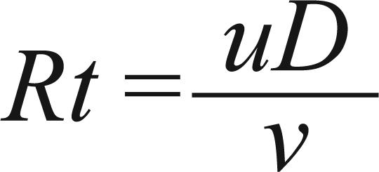

Because the changing trap diameter (D) affects the trap Reynolds number (Rt) and cone trap aspect ratio (Ac), only one dimensionless parameter should be altered when testing for the dependence between each parameter and the trapping efficiency. Because Rt and Ac are closely linked, we treated them both together. We predicted the theoretical trap efficiency as a function of varying Rt while holding Ac constant for the conical trap geometry.

RESULTS AND DISCUSSION

The Numerical Model

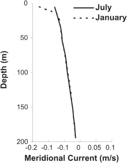
Hydrodynamic model MOM represented the main features of the meridional current in the study area and indicated that the mean flow varies both spatially and temporally. However, because of our use of monthly data rather than daily data, our results were lower than the in situmeasurements. The vertical structure of the meridional current component at parallel 23° S presented a similar propagation direction with a difference in intensity near the surface from the shear stress in January as generated by the occurrence of stronger northeast winds (Figure 3). Close to the surface (5 m depth), the maximum velocity (-0.13 m/s) occurred in a southwards direction in January; after a decline in the flow (-0.07 m/s), a smooth decreasing trend towards the sea floor (-0.01 m/s) was found. The current decreased in July, with values varying from -0.08 to -0.01 m/s. In January, the velocity component related to the SACW was more evident on the continental shelf in comparison to that of July, probably because of the stronger northeast winds. This seasonal pattern has been previously documented and the SACW has been shown to proliferate at shallower depths during the austral summer and deeper depths during the austral winter (Candella 1999).

Figure 3 -
Modular Ocean Model output of the vertical profiles for the meridional current velocity (North-South) for one point on the grid near the mooring position off the Brazilian coast (23° S) during January and July from 1963 to 2003.

The Dynamic Design

The effects of the equipment and mechanical instrument weights on the mooring line were expressed by Matlab as the vertical load (Table I). The array had a high vertical load (350 kg) because of the several assembled pieces of oceanographic equipment along the mooring line. The Muringa model had the potential to predict if the array was subject to a risk of displacement from the total drag by the currents. The low drag (16 N) recorded for the array reflected an insignificant effect on the maximum surface current under consideration (0.5 m/s), as generally found along the Brazilian coast and BC.

TABLE I
Parameter outputs of the Matlab and Muringa modeling considering a maximum velocity of 0.5 m/s.

Models	Parameter Outputs	Units	Cabo Frio Array (23° S)
Matlab	Current velocity	m/s	0.5
	Vertical load	kg	350
	Horizontal load	kg	71
	Tilt	degree	2.6 ± 0.6
	Tension on anchor	kg	350
	Safe wet anchor mass	kg	578
	Safe dry steel anchor mass	kg	665
	Safe dry concrete anchor mass	kg	890
Muringa	Total drag	N	16
	Tilt	degree	2.1 ± 0.7
	Tension on anchor	N	4470
	Safe wet iron anchor mass	kg	456
	Safe dry iron anchor mass	kg	514

Figure 4 summarizes the buoyancy of the buoys and the tension elements calculated by Muringa for the array. Along the array, both the buoyancy of the buoys and the tension element increased with depth, with only a smooth decrease at the seafloor, especially when floats were present. Because the drag on the cable was added to the element immediately above, the effort remained concentrated on this element and changed only when the next component was added. The total buoyancy of the buoys was 456 kg (Figure 4) and was related to a minimum anchor wet weight of 456 kg for Muringa (iron material) and 665 kg for Matlab (steel material) (Table I). Our results indicate that the mooring had a well-distributed backup flotation device for emergency recovery purposes (e.g., if the mooring snapped along any part on the mooring line). Assuming a 2-fold security factor, the recommended anchor wet weight ranged from 912 kg to 1330 kg.

Figure 4 -
Muringa modeling of the buoyancy summary and tension element attesting to the correct distribution of the buoys for the maintenance of the mooring array tension.

The increased weight of the mooring with depth must be supported by the buoy system and this trend has implications for drag determinations, since the tilt angle is sensitive to the total weight. From the Matlab model of the array, we can also conclude that the backup flotation device resulted in a more stable mooring; the effect of the surface current (0.5 m/s) on the mooring tilt angle was low (2.6° ± 0.6) (Table I, Figure 5).

Figure 5 -
Output from Matlab modeling forced by a surface velocity current of 0.5 m/s attesting the low tilt of the mooring line in Cabo Frio.

Taking into account different modeling programs (Matlab, Muringa and MOM), the design criteria identified complementary safety factors for trap deployment and particle trapping. The criterion based on extreme environmental conditions (e.g., swells, cold fronts) resulted in designs with varying safety levels. Hence, the design criteria based on maximum environmental conditions seemed to be an effective methodology for safely operated current mooring designs over the one-year field exposure experiment.

Trap Efficiency

Tilt is a function of the dynamics of a complete mooring (Gardner 1985, Buesseler et al. 2007). Conical traps with an aspect ratio (Ac) of 1.75 were tilted from 1° to 2.8° in the mooring line with currents of 0.5 m/s at 43 m and 109 m depth (Table II). Conical trap collection efficiency declines with increased tilt. Our calculated tilt was minor and had a negligible bias, indicating that the mooring line fulfilled the requirements of axial symmetry (GOFS 1989), and thus remained in a vertical position. The mechanism by which particles are retained inside traps allows increased particle retention until Ac is sufficiently large, after which the dynamics of particle retention are held constant (GOFS 1989). Considering the deployment off Cabo Frio, the major diameter opening of the conical trap (660 mm diameter) was necessary for collecting larger particles in this relatively low productivity area. The advantage of the McLane trap design with a 41° cone-angle is that the sloping wall decreases the updraft of fluid moving over the container (Gardner 1980). Additionally, a baffle composed of short cells with a 1″ diameter was used to reduce the rate of turbulence and mixing at the top of the cones. However, it has been shown that cone baffles whose cells where 3/8″ wide and 2″ high reduced the primary circulation at the top of the cone but they did not eliminate it completely (Gardner 1980). Baffled cones with an Ac of ∼1 trapped fewer particles, especially fine particles (Gardner 1980, 1985), but tests have not been conducted using larger cones with an Ac of ∼2 (Honjo and Doherty 1988), such as the one we used in Cabo Frio (Table II).

TABLE II
Trapping efficiency of the sediment trap evaluation. Abbreviations: h, height of the trap; d, top diameter of the trap.

Trap Type	Depth [m]	Angle Top - Bottom [°]	h/d Ratio	Current Velocity [m/s]	Reynolds Number
					TW (25° C)
				max 0.50	2×105
Mark-8	Top	1.0 - 1.9	1.75	mean 0.30	1×105
Conical	25			min 0.15	5×104
					SACW (15° C)
				max 0.50	2×105
Mark-8	Bottom	2.7 - 2.8	1.75	mean 0.30	1×105
Conical	91			min 0.15	4×104

The Reynolds number (Rt) for conical traps ranged from 4 × 10⁴ to 2 × 10⁵ for current velocities between 0.1 and 0.5 m/s, respectively (Table II). These Rt values are similar to those found by Gust et al. (1992) for conical traps, where higher velocities were concomitant with higher registered mass fluxes. In fact, the conical trap geometry is advantageous for collecting and concentrating large samples (GOFS 1989). In general, the conical trap provided reasonable particle interception efficiency. A less efficient particle trap is explained by a more turbulent exchange of water and particles between the interior and exterior of the trap in flowing water (Bale 1998). Moreover, trapping efficiencies should not be considered to be controlled by hydrodynamic conditions alone. The efficiencies are affected by interactions between the hydrodynamic conditions and the sinking particle properties (e.g., density, size, form and sinking rates) (Buesseler et al. 2007).

Lau (1979) and Butman et al. (1986) discussed the relationship between Ac and Rt for cylindrical traps and indicated the existence of processes that caused an approximate separation between captured and escaped (partially captured) material. They suggested that only traps with an Ac of 2.25 and an Rt of 1 × 10⁴ would retain material. For retaining material in oceanic conditions that have relatively high Rt values (> 10⁵), it is necessary to use a cylindrical trap with an Ac of ∼9. The trapping efficiency of cones as a function of Ac and Rt has not been empirically determined (Butman et al. 1986, Asper 1996, Honjo 1996).

CONCLUSIONS

Taking into account the use of the Matlab and Muringa modeling programs, the design criteria assured detailed computations for the optimization of the total weight, the buoyancy balance, and the maximum acceptable tilt to avoid hydrodynamic bias upon the trapping efficiency. With the MOM model, estimates of the meridional current component were performed to assist in the adaptation of the array to the local oceanographical conditions. Hence, the three modeling tools identified some of the crucial safety factors needed for the deployment and particle trapping efficiency of the array. After the precautionary analyses, the mooring array was successfully deployed at the shelf edge off Cabo Frio, being a stable platform which could be safely operated during several events over a one-year field study period.

This project was financially supported by the Geochemistry Network from PETROBRAS/CENPES and by the National Petroleum Agency (ANP), Brazil (Grant 0050.004388.08.9). A.L.S Albuquerque and B.A. Knoppers are senior scholars from the Conselho Nacional de Desenvolvimento Científico e Tecnológico (CNPq, Brazil). We are in debt to the anonymous reviewer whose indepth analysis and many suggestions contributed significantly to this manuscript.

REFERENCES

• Albuquerque AL, Belem AL, Zuluaga FJB, Cordeiro LG, Mendoza UN, Knoppers BA, Gurgel MHC, Meyers PA and Capilla R. In Press. Particle fluxes and bulk geochemical characterization on the Cabo Frio Upwelling System in, Southeastern Brazil: Sediment Trap Experiments between Spring 2010 and Summer 2012. An Acad Bras Cienc.
• Asper VL. 1988. A review of sediment trap technique. Mar Technol Soc J 21: 18-25.
• Asper V. 1996. Particle flux in the Ocean: Oceanographic Tools. In: ITTEKKOT V ET AL. (Eds), Particle Flux in the Ocean, SCOPE 57, Chichester: Wiley & Sons, Chichester, England, p. 71-84.
• Assad LPF, Candella RN and Torres Junior AR. 2008. Características climatológicas do Oceano Atlântico Sul obtidas a partir de um Modelo Computacional Global (MOM). Pesq Nav (SDM) 21: 17-25.
• Assad LPF, Torres Jr AR, Zumpichiatti WA, Mascarenhas Jr AS and Landau L. 2009. Volume and heat transports in the world oceans from an ocean general circulation model. Braz J Geophys 27: 181-194.
• Bale AJ. 1998. Sediment trap performance in tidal waters: comparison of cylindrical and conical collectors. Cont Shelf Res 18: 1401-1418.
• Belem AL, Castelao RM and Albuquerque ALS. 2013. Controls of subsurface temperature variability in a western boundary upwelling system. Geophys Res Lett 40: 1362-1366.
• Buesseler KO, Antia AN, Chen M, Fowler SW, Gardner WD, Gustafsson O, Haranda K, Michels A, Loeff Van Der MR and Sarin M. 2007. An assessment of the use of sediment traps for estimating upper ocean particles fluxes. J Mar Res 65: 345-416.
• Butman CA, Grant WD and Stolzenbach KD. 1986. Predictions of sediment trap biases in turbulent flows: a theoretical analysis based on observations from the literature. J Mar Res 44: 601-644.
• Campos EJD, Velhote D and Silveira ICA. 2000. Shelf break upwelling driven by Brazil Current cyclonic meanders. Geophys Res Lett 27: 751-754.
• Candella RN. 1999. Correlação temperatura x salinidade e variação sazonal da água central do Atlântico Sul no quadrado de Marsden 376. Pesq Nav (SDM) 12: 35-39.
• Carbonel AAH. 2003. Modeling of upwelling-downwelling cycles caused by variable wind in a very sensitive coastal system. Cont Shelf Res 23: 1559-1578.
• Castelao RM. 2012. Seasurface temperature and wind stress curl variability near a cape. J Phys Oceanogr 42.
• Castelao RM and Barth JA. 2006. Upwelling around Cabo Frio, Brazil: the importance of wind stress curl. Geophys Res Lett 33.
• Castro BM and Miranda LB. 1998. Physical oceanography of the western Atlantic continental shelf located between 4° N and 34° S. In: ROBINSON AR ET AL. (Eds), The sea, New York: Wiley, New York, USA, p. 209-251.
• Chaplin CR. 1999. Torsional failure of a wire rope mooring line during installation in deep water. Eng Fail Anal 6: 67-82.
• Chavez FP and Toggweiler JR. 1995. Physical estimates of global new production: the upwelling contribution. In: SUMMERHAYES CP ET AL. (Eds), Upwelling in the Ocean: Modern Processes and Ancient Records, New York: J Wiley & Sons, New York, USA, p. 313-320.
• Dewey RK. 1999. Mooring design and dynamics – a Matlab package for designing and analysing oceanographic moorings. Mar Model 1: 103-157.
• Fischer G et al. 2009. Mineral ballast and particle settling rates in the coastal upwelling system off NE Africa and the South Atlantic. Int J Earth Sci 98: 281-298.
• Gardner WD. 1980. Field assessment of sediment traps. J Mar Res 38: 41-52.
• Gardner WD. 1985. The effect of tilt on sediment trap efficiency. Deep Sea Res 32: 349-361.
• Griffies SM et al. 2005. Formulation of an ocean model for global climate simulations. Ocean Sci 1: 45-79.
• Gust G, Byrne RH, Bernstein RE, Betzer PR and Bowles W. 1992. Particle fluxes and moving fluids, experience from synchronous trap collections in the Sargasso Sea. Deep Sea Res I 41: 831-857.
• GOFS. 1989. Sediment trap technology and sampling, Report of the U.S. GOFS Working Group on Sediment Trap Technology and Sampling. U.S. Planning Report No 110, 94 p.
• Honjo S. 1996. Fluxes of particles to the interior of open oceans. In: ITTEKKOT V et al. (Eds), Particle Flux in the Ocean, SCOPE 57, Chichester: J Wiley & Sons, Chichester, England, p. 91-154.
• Honjo S and Doherty KW. 1988. Large aperture time-series oceanic sediment traps: design, objectives, construction and application. Deep Sea Res 35: 133-149.
• Honjo S, Spencer W and Gardner WD. 1992. A sediment trap intercomparison experiment in the Panama Basin. Deep Sea Res 39: 333-358.
• Lau YL. 1979. Laboratory study of cylindrical sedimentation traps. J Fish Res Bd Can 36: 1288-1291.
• Moreira da Silva PC and Rodrigues RF. 1966. Modificações na estrutura vertical das águas sobre a borda da plataforma continental por influência do vento. Publicação do Instituto de Pesquisa da Marinha, Arraial do Cabo, Rio de Janeiro, Brasil 96: 56.
• Murray RJ. 1996. Explicit generation of orthogonal grids for ocean models. J Comput Phys 126: 251-273.
• Pacanowsky RC and Griffies SM. 1999. The MOM3 manual. Geophysical Fluid Dynamics Laboratory/NOAA, Princeton, USA, p. 680.
• Pilskain CH, Paduan JB, Chavez RY, Anderson RY and Berelson WM. 1996. Carbon export and regeneration in the coastal upwelling system of Monteray Bay, central California. J Mar Res 54: 1149-1178.
• Rodrigues RR and Lorenzzetti JA. 2001. A numerical study of the effects of bottom topography and coastline geometry on the Southeast Brazilian coastal upwelling. Cont Shelf Res 21: 371-394.
• Röeske F. 2001. An atlas of surface fluxes based on the ECMWF reanalysis: A climatological dataset to force global ocean general circulation models. Max Planck Institut für Meteorologie, Hamburg, Germany, Report No. 323.
• Roughan M and Middleton JH. 2002. A comparison of observed upwelling mechanisms off the east coast of Australia. Cont Shelf Res 22: 2551-2572.
• Senger JV and Watson JTR. 1986. Improved international formulations for the viscosity and thermal conductivity of water substances. J Phys and Chem Ref Data 15: 1291-1314.
• Smith NP. 1983. Temporal and spatial characteristics of summer upwelling along Florida's Atlantic shelf. J Phys Oceanogr 13: 1709-1715.
• Suess E. 1980. Particulate organic carbon flux in the ocean-surface, productivity and oxygen utilization. Nat 288: 260-263.
• Sun C, Rieneker MM, Rosati A, Harrison M, Wittenberg A, Keppenne CL, Jacob JP and Kovach RM. 2007. Comparison and sensitivity of ODASI ocean analyses in the tropical Pacific. Mon Weather Rev 135: 2242-2264.
• Tsinker GP. 1994. Marine structures engineering: specialized applications. New York: Chapmann & Hall, New York, USA, p. 544.

Publication Dates

• Publication in this collection
  June 2014

History

• Received
  16 July 2012
• Accepted
  10 July 2013