Numerical Study of Wake Characteristics in a Horizontal-Axis Hydrokinetic Turbine

ABSTRACT

Over the years most studies on wake characteristics have been devoted to wind turbines, while few works are related to hydrokinetic turbines. Among studies applied to rivers, depth and width are important parameters for a suitable design. In this work, a numerical study of the wake in a horizontal-axis hydrokinetic turbine is performed, where the main objective is an investigation on the wake structure, which can be a constraining factor in rivers. The present paper uses the Reynolds Averaged Navier Stokes (RANS) flow simulation technique, in which the Shear-Stress Transport (SST) turbulent model is considered, in order to simulate a free hydrokinetic runner in a typical river flow. The NREL-PHASE VI wind turbine was used to validate the numerical approach. Simulations for a 3-bladed axial hydrokinetic turbine with 10 m diameter were carried out, depicting the expanded helical behavior of the wake. The axial velocity, in this case, is fully recovered at 12 diameters downstream in the wake. The results are compared with others available in the literature and also a study of the turbulence kinetic energy and mean axial velocity is presented so as to assess the influence of proximity of river surface from rotor in the wake geometry. Hence, even for a single turbine facility it is still necessary to consider the propagation of the wake over the spatial domain.

Key words:
hydrokinetic turbines; wake characteristics; CFD; turbulence

INTRODUCTION

There is no doubt that Brazil has an enormous watershed and relevant river connections, which provide an important hydraulic energy source for its territory, ensuring hydraulic energy as the most representative power source of the country. Although the Amazon region presents a great part of such hydraulic potential due to rivers being highly connected and having high flow rates, it is still largely unused for hydrokinetic energy purposes. Taking advantage of the water velocity (hydrokinetic energy) so as to convert it into electrical energy, seems to be more suitable than utilizing traditional hydraulic turbines, which need, in general, huge heads to convert potential energy into electricity.

Hydrokinetic turbines have recently been used as converters of river, tidal and marine currents into electrical energy. This technology has become significant due to the use of renewable energy sources with low environmental impact and do not require large civil structures, making this technology an attractive alternative to conventional hydropower (Schleicher et al. 2015). Mesquita et al. 2014 present a general methodology for the efficient design of horizontal-axis hydrokinetic turbines with variable rotation. Their model includes the effect of multiplier, electric generator, inertia of whole system, and frictional resistances of a turbine with a 10 m diameter and producing electric power of around 500 kW. Churchfield et al. 2013 describes an important application of the six marine turbine with 5 m diameter placed in an array in the East River in New York City and a dual rotor in Strangfordlough in Nothern Ireland converting 1,2 MW.

Hydrokinetic and wind turbines are very similar devices regarding the theoretical aspects of the fluid mechanics related to them. In spite of the difference of fluid, several models have been developed for different configurations, such as free flow and adapted with diffuser technology (Barbosa et al. 2015), which have been applied in both turbines. Consequently, extensive work has been carried out on the wake characteristics of horizontal axis wind turbines (Chamorro and Porté-Agel 2009, Gómez-Elvira et al. 2005, Vermeer et al. 2003). Therefore, in general, wake studies are mainly concerned with wind turbines and there are few works related to wake in hydrokinetic turbines (Gant and Stallard 2008, Harrison et al. 2010, MacLeod et al. 2002) especially in rivers, since depth and width are limited parameters. Such analysis is a relevant contribution to the turbines in array along the rivers, once the rotor wake structure of the first turbine promotes a significant influence on the subsequent turbine performance, decreasing the power production. In this regard, the knowledge of the wake characteristics in multi-turbine arrays becomes very important in order to improve the output power produced.

The action of the turbine on the flow causes a disturbance in the region downstream of the rotor, characterized by intense turbulent mixing, helical movements and a complex eddy system. In turbomachinery this region is called wake. Much of this complexity arises from the adverse pressure gradient at the rotor plane, which contributes to instability of boundary layers along the blades. Additionally, a spiral vortex structure is shed outwards from the blade tips and the rotor root, producing large eddy structures which last for a long time in the flow. Vermeer et al. 2003 bring a detailed overview on the wake structure of wind turbines, in which some of the most basic aerodynamic mechanisms governing the power output are not yet fully understood. From the perspective of turbine farm layouts, there are two main characteristics of the wake: (a) velocity deficit downstream, which is related to the rotor power conversion; (b) turbulence levels, which can affect the induced flow on other turbines situated downstream (Chamorro and Porté-Agel 2009).

Thus, the goal of this paper is to perform a numerical investigation of the wake characteristics on a horizontal-axis hydrokinetic turbine using the Computational Fluid Dynamics (CFD) technique, including detailed features of near and far wake at high tip speed ratios. The methodology applied in all simulations was based on the Unsteady Reynolds Averaged Navier Stokes (URANS) technique and the Shear-Stress Transport (SST) turbulence model, performed by ANSYS CFX software. The numerical validation was achieved using a 2-bladed axial wind turbine NREL-PHASE VI, which was tested in the 24 x 36 m NREL/NASA Ames wind tunnel (Hand et al. 2001, Simms et al. 2001). The numerical simulations for a single 3-bladed hydrokinetic turbine were carried out, depicting the expanded helical behavior of the wake. The radial expansion of the wake is 1.2R of radius in a helical cylinder along the whole near wake. The axial velocity, in this case, is fully recovered at 12 diameters, marking the end of the far wake. Results show that for multiple hydrokinetic turbines it is necessary to consider the spread of the wake over the spatial domain. Furthermore, an overview of the turbulence characteristics downstream of the rotor is carried out, including temporal and spatial evolution of the axial normalized velocity at the wake. The understanding of the wake development and its dissipation is critical to the ideal arrangement of hydrokinetic turbines in rivers.

The flow behavior in the wake is quite peculiar, and follows a sequence of phenomena as illustrated in Figure 1. The wake behind the turbine is mainly classified as near wake and far wake. While in the former, the wake features directly affects the flow with sharp gradient velocity and a peak of turbulence intensity due to complex vortex structures, the latter provides a recovery of velocity and a fall of the overall turbulence intensity (Sanderse 2009). In this sense, as the flow approaches the rotor, the stream velocity decreases and the pressure rises. However, as soon as it goes through the rotor, the pressure drops dramatically and hits the lowest level. Immediately after leaving the rotor plane, the velocity and pressure fields become non-uniform, as a consequence of the rotor action over the flow. The non-uniformities of the velocity field are related to the vortex shedding from the rotating blades (Gomez-Elvira et al. 2005). As it moves downstream, the influence of the wake expands radially, the velocity on the wake decreases and the local pressure increases sharply until reaching the ambient pressure, which marks the end of the near wake and the beginning of the far wake in approximately 5 diameters (Manwell et al. 2002, Vermeer et al. 2003).

Figure 1
Schematic representation of the turbine wake. Adapted from Sanderse 2009.

After this point, the presence of the rotor is no longer predominant and the turbulence acts as an efficient mixer, dominating the physical process. As a result of this process, far downstream of the rotor, the velocity profile becomes approximately Gaussian and the axial velocity rises slowly approaching the non-disturbed velocity (Sanderse 2009, Vermeer et al. 2003). Besides these two well-defined regions, Brand (2011), Eecen and Bot (2013), Frandsen and Barthelmie (2002), Werle (2008) identifies a transition zone, called intermediate wake. In that region, the turbulent diffusion begins with the interaction between the wake and the undisturbed flow. The wake tip vortices then steadily lose their identity and the turbulent mixing concentrates in an annular shaped shear layer at the boundary of the wake. As a result, turbulence starts to fall (Brand 2011, Eecen and Bot 2013).

NUMERICAL METHODOLOGY

The flow is assumed to be incompressible and fully turbulent. Consequently, velocity and pressure fields are governed by the Navier-Stokes equations. In order to consider the turbulent phenomena without numerically solving all the eddy scales, the Reynolds Averaged Navier-Stokes (RANS) approach was adopted. In this manner, the governing equations of the flow are the continuity and momentum conservation equations that can be described, respectively, as

(1)

(2)

where u_i are the components of the velocity, ρ is the density, p is the mechanical pressure, µ is the viscosity and f_j is a force per unit of volume which may represent the Coriolis and centrifugal contributions, for example. In this methodology, the contribution of the turbulent velocity fluctuations u_i to the temporal average velocity and pressure fields are given by the Reynolds Stress Tensor Davidson 2004, Pope 2000). There are several numerical models available in the literature to perform this task, as can be seen in Wilcox 1988, and more recently Argyropoulos and Markatos 2015. In the present work, the so-called Κ-ω Shear-Stress Transport (SST) model, in the form it was described by Menter 1993, 1994 is employed. The SST model was developed to give an answer to the necessity of models which can handle aeronautical flows with strong adverse pressure gradients and separation of the boundary layers. For that, SST combines the Κ-ω model in regions near to the solid walls, with Κ-ε for the free-stream ow out of the boundary layers. This is possible due to the definition of auxiliary switch functions, which mainly depends on the turbulent quantities and the dimensionless normal distance from the wall. Thereby, Κ-ω calculates the turbulent contribution from the inner boundary layers without any extra damping functions. Besides that, Κ-ε takes place out of the boundary layers, avoiding the excessive sensitiveness of the Κ-ω model to the inlet free-stream conditions. Therefore, the SST model has been found to give very good results for wall-bound flows, even in cases of highly separated regions as typically found in axial turbines as reported by Mo and Lee 2012, Moshfegh and Xie 2012 and Menter et al. 2003. In this sense, it is a natural choice for numerical simulation of flows through hydrokinetic turbines, which has a similarity of operation with wind turbines., which must be modeled (

Conventionally, in RANS calculations, the steady-state solution is the main goal, as the time-averaged Navier-Stokes equations are solved. Nevertheless, as the time interval used for the time averaging of the Navier-Stokes is reduced, and the transport equations are solved as dependent on time, an unsteady RANS scheme can be obtained. The simulations of this work were carried out using ANSYS CFX, which is a commercial CFD code based on the finite-volume method with an unstructured parallelized coupled algebraic multigrid solver with a second order advection scheme and second order overall accuracy. In addition, the unsteady terms in the governing equation are solved using an implicit second order backward time-stepping algorithm, in which the variables computed in each time-step are based on the result of the previous time interval and the estimative of the following one.

An unstructured and hybrid mesh was used in all simulations in order to achieve better results with less computational power available. In general, the flow domain was mainly composed by tetrahedron elements, since they are highly adaptive for complex geometry and large grid deformation, which represent a great cost/benefit concerning the size and numerical quality of the mesh for this problem (Freitag and Ollivier-Gooch 2000, Wu et al. 2001). Nevertheless, in the boundary layer, which is the near region of the blade surface, prismatic elements are commonly used. This type of computational mesh is recognized to be able to accurately compute the viscous forces of the boundary layer (Garimella and Shephard 1998). Since the flow on this region is defined by the alignment with the solid surface and a high velocity gradient in the normal direction, the parallel bases of the prism allows that mesh to always be aligned to the solid surfaces as well. Furthermore, due to its shape, the element aspect ratio can be adjustable to reach large bases and short heights without a decrease in the mesh quality, so as to deal with a different gradient in each direction.

It is well known that a common parameter to identify the subparts of the boundary layer is the dimensionless distance from the wall ^_y+ (Wilcox 1988), defined by ^_u+ is the wall shear velocity. In this manner, the near-wall region can be roughly subdivided into three layers: viscous layer (^_y+ < 5), buffer layer (5 < ^_y+ < 30) and the fully turbulent layer (^_y+ > 30) (Schlichting et al. 2000). Consequently, to solve the viscous sublayer, the values of ^_y+ in the simulation must be suitable to the turbulence model employed, in this case y⁺ < 1 which allows the solution of laminar sub-layer by the SST Κ-ω turbulence model., where

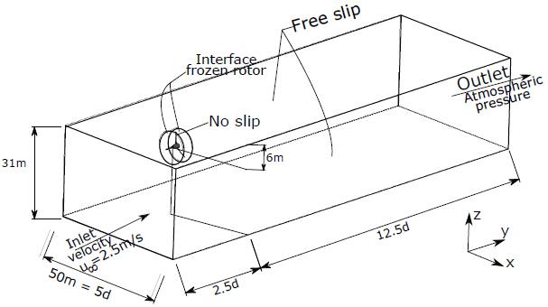
A 3-bladed hydrokinetic rotor with a 10 m diameter was virtually constructed based in NACA 65₃ - 618 airfoil with a nonlinear twist distribution. The computational domain is a parallelogram with dimensions 31 m x 50 m x 150 m as illustrated in Figure 2. The computational domain was divided in two parts: rotating and stationary. The first part has the shape of a cylinder with a 6 m radius and a 3 m length. The other part has a box format, which has a length of 45 m and also contains the rotating sub-domain. The rotor is positioned at 2.5 diameters from the inlet boundary and 12.5 rotor diameters from the outlet, in order to avoid any spurious influence of these boundary surfaces. The hydrokinetic turbine center was placed at 6 m from the river surface (H = 6 m).

Figure 2
Setup of the computational domain (Silva et al. 2016).

In contrast to the hydrokinetic case, in the NREL PHASE VI validation the domain was shaped so as to be similar to the experiments. In this manner, the parallelogram has 45 m of height and width and 60 m of length. The turbine was placed at a 15 m boundary from the upwind and top surfaces so as to avoid spurious influences of the inlet and outlet sections.

The boundary conditions were applied in the computational domain in order to accurately represent the turbine operation in the wind tunnel and river as follows:

• Inlet velocity: a Dirichlet boundary condition which is assigned the uniform velocity in the normal face with turbulence intensity of 5%. In this manner, the pressure is determined in a way to satisfy transport equations.

• Outlet pressure: in the upwind face another Dirichlet boundary condition was applied so as to define the atmospheric pressure (101325Pa). Therefore, the velocity field is evaluated in the in order to satisfy transport equations.

• Non Slip: applied to the rotor surface, implying that the relative velocity of the fluid particle on the solid surface is zero.

• Free Slip: imposed in the wind tunnel wall so as not to affect the flow. In this way, the shear stress between the tunnel wall and fluid is zero.

• Interface: in RANS simulations a rotational reference frame was imposed inside the cylindrical subdomain in order to save computational resource by converting inherently transient ow into steady state. In this way, the rotor is kept in a fixed position and the governing equations are solved considering a modified gravitational acceleration, taking into account the Coriolis and centrifugal components. However, in URANS simulations a true transient method was applied by a sliding mesh condition.

RESULTS AND DISCUSSION

NUMERICAL VALIDATION

For years the empirical complexity and instrumental uncertainty had inhibited an achievement of consistent experiments which demonstrates clearly the physics and operation of turbines. The analysis of real scale turbines requires huge technical devices and high quality instrumentation (Schreck 2002). Even with the recent technological advances in the last decades, real scale experiments were nearly nonexistent. This challenge led the National Renewable Energy Laboratory (NREL) to design the Phase VI turbine and test it in the NASA/ASME 24.4 x 36.6 m wind tunnel. The results of this analysis represent a benchmark in the evaluation of the performance of numerical codes around the world and a gain in knowledge regarding turbine aerodynamics (Hand et al. 2001, Simms et al. 2001).

The NREL Unsteady Aerodynamics Experiment Phase VI was performed using a 10.58 m diameter, 2 blades, twisted, stall regulated wind turbine. The blade geometry was based in the airfoil S809 with a nonlinear twist distribution. Pressure sensors were placed in five radial positions (0.3R, 0.47R, 0.63R, 0.8R and 0.95R) with the purpose to evaluate in detail the pressure field on the blade. Moreover, wake measurements were made by two sonic K anemometers placed 2 m from each other and both located at 5.84 m in the axial direction. Full information of the experimental results including the test plan, geometry, instrumentation, and calibration are clearly exposed by Hand et al. 2001. Among all experiment configurations in this work, the following case was considered: 5-20 m/s wind velocity, global pitch and yaw angles set in 5° and 0°, respectively, and rotational speed fixed at 72 rpm.

A large computational domain and different phenomena in many regions allow a number of possibilities of mesh refinement configurations. The region near the blade plays a key role on the turbine operation, since it has the highest gradient of static pressure and velocity. On the other hand, the near wake flow, which can extends up to 3D downstream the rotor, has also a great effect on the power (Moshfegh and Xie 2012). The refinement in the boundary layer and a sensitivity study of ^_y+ is equally important as the near wake region, since both can directly affect on turbine aerodynamic, especially in an operational range of Tip Speed Ratio (TSR) which has both separated and attached ow.

In order to overcome this mesh arrangement issue, the grid independence study started with a good definition of the boundary layer and a coarse refinement in the wake. The results were compared to the experimental data of Simms et al. (2001) for Table I. To assess the resolution of the boundary layer, the dimensionless distance from the wall (Wilcox 1988), defined by ^_u+ is the wall shear velocity, and v is the kinematic viscosity. To solve the viscous sublayer of the Κ-ω SST turbulence model, the values of ^_y+ generally must be less than 1 (Schlichting et al. 2000). Following meshes were made by increasing the refinement of the near wake and achieving a good resolution of the boundary layer. Mesh 3 reached a convergence of results with 8 106 nodes and 3.3 % error on power. In this way, a further refinement might not improve the numerical results. The computed power has also presented a good agreement with several results available in the literature, as depicted in Figure 3., as shown in was used, where is the distance of the first node from the wall,

TABLE I
Mesh Independence study.

Mesh	Nodes [x 106]	Wake Refinement [m]		Power [kW]	Error %
Mesh 1	1.98	23	0.221	5.2	13
Mesh 2	6.28	23	0.268	6.4	7
Mesh 3	8.12	23	0.250	5.8	3.3

Figure 3
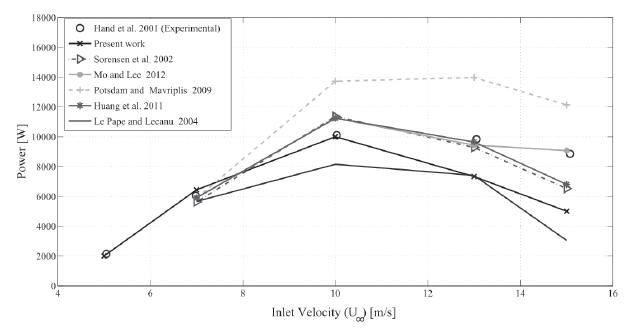
Output Power as a function of Inlet Velocity: Comparison with results available in the literature.

The power as a function of the inlet velocity, obtained using Mesh 3, was compared with several results available in the literature, as depicted in Figure 3. The present work has good agreement with other numerical investigations, which spread out around the experimental reference. In particular, for 10 m/s, the present simulation predicts exactly the experiment's results. However, for higher velocities (13 and 15 m/s), in which the boundary layers are completely collapsed, the numerical error in the present work rises because of the inability of SST turbulence model to predict it accurately Mo and Lee 2012.

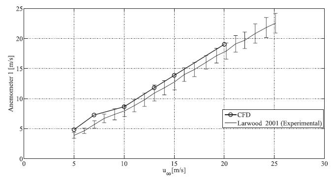
In order to present a local validation of the wake flow simulation, the numerical velocity data were compared with the experimental data published by Larwood 2001. Figures 4 and 5 show the velocity profile in the wake, which presents a remarkable agreement with the experiments if the uncertain data are taken into account. Since, in most of cases, it stays inside the interval defined by the error bars.

Figure 4
Comparison between numerical and experimental (Larwood 2001) velocities - anemometer 1.

Figure 5
Comparison between numerical and experimental (Larwood 2001) velocities - anemometer 2.

A steady-state simulation was performed for approximately 1500 iterations so as to reach a convergence both in power values and in residual variables below 10^-3. Afterwards, the numerical result was used as an initial condition to the unsteady simulation having a residual of 10^-3, which is restrictive enough to achieve results compatible to the ones obtained by Mo et al. 2013. In this phase, a time-step of 0.1 s and a total simulation time of 30 s were set, sufficient for the rotor to perform 36 rotations.

WAKE CHARACTERISTICS OF THE HYDROKINETIC TURBINE

The mesh refinement study was performed following the same criteria exposed in the validation case. As is shown in Table II the convergence of numerical results was obtained in the Mesh C, in such a way that a further mesh refinement was no longer necessary. Similarly to the NREL PHASE VI simulations, the unsteady simulation was carried out using the steady state flow solution as a starting condition. However, here a time-step of 0.3 s and a total simulation time of 40 s were used, which corresponds to 23 complete rotations of the turbine.

TABLE II
Mesh refinemente study.

Mesh	Nodes [x 106]		Power [kW]
Mesh A	4.3	1.54	291
Mesh B	7.5	1.07	255
Mesh C	8.5	1.20	251

Figure 6 shows the deficit of the axial velocity downstream in four times (20, 30, 35 and 40 s), where the time evolution and the propagation of the wake over the domain can be seen. The spatial and time convergence of the normalized axial velocity is also noteworthy, which is firstly verified near the turbine (0 ?λτ; y / D ?λτ; 4)) and then at regions far from the rotor. Conversely to the inviscid Axial Momentum Theory Wilson and Lissaman 1978, in actual flows the non-disturbed free stream speed is recovered due to action of the molecular and, mainly, turbulent diffusion, as well as the complex transport phenomena which takes place at the rotor wake. Note that the normalized axial velocity is completely recovered around 12D (meaning 12 times the rotor diameter).

Figure 6
Time evolution and spread of the wake.

Figure 7 gives information about the normalized axial velocity, turbulence kinetic energy (TKE) and the relative pressure downstream. Note that in the rotor axis line () a sharp fall in the velocity due to the presence of the nacelle can be seen. However, this effect is suddenly dissipated and at two diameters tend to follow the same pattern of other radial positions (r/R). Another parameter that causes a great effect in the wake is the proximity between the rotor and the river surface, since the flow velocity is increased by the presence of the free-surface. As a free slip condition was imposed in this face, the wake has a greater propagation in the axial direction. This is evident from the curves and , which shows a slow recovery for the first curve when compared with the second curve. However, some phenomena need to be considered in this work, e.g., the surface waves change the profile of turbulent intensity and the turbulence kinetic energy due to the effect of two different fluids, air and water, which probably modifies the wake structure for hydrokinetic turbines. Such concerns present complexity and more investigations are being conducted. Regarding the turbulence kinetic energy (TKE), the inlet boundary condition has a small influence on the flow with a slight increase, however this effect rapidly disappears as a consequence of the rotor disturbance in the flow, which is much more appreciable. Downstream of the turbine, the TKE rises substantially owing to the tip blade vortex formation and shedding. Shortly thereafter, the TKE plunges around due to instability and collapse of the vortex (Chamorro and Porté-Agel 2009), indicating the end of the near wake. It is also noticed, in the pressure curve at immediately after the TKE decay, that the relative pressure achieves the reference pressure, which is the main characteristic of the end of the near wake (Gomez-Elvira et al. 2005).

Figure 7
(a) Mean axial velocity, (b) turbulence kinetic energy (TKE) and (c) relative pressure downstream.

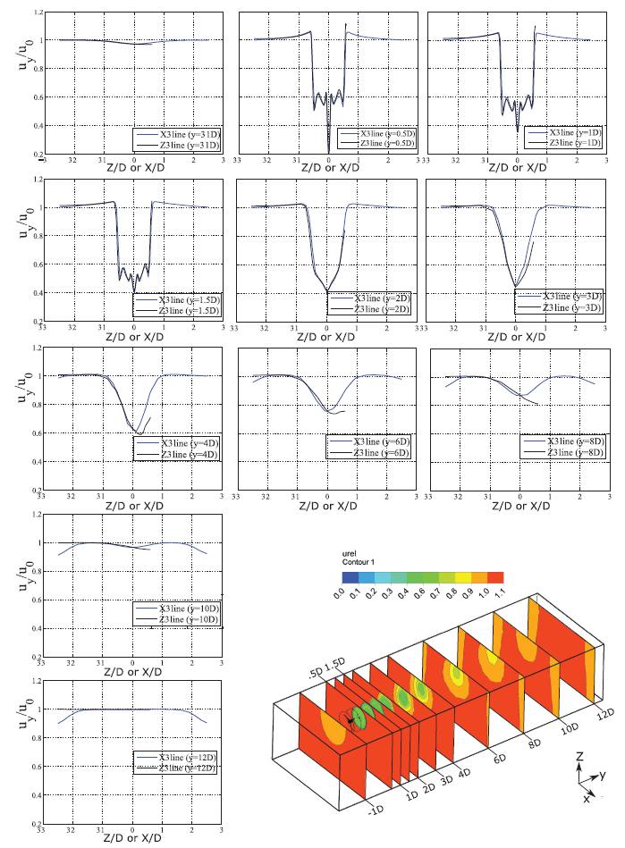
In order to evaluate the dimensions of the stream tube which encloses the wake, the computational domain was sectioned in planes parallel to the rotor plane as depicted in Figure 8. For this analysis, the normalized axial velocity deficit was presented in two ways: graphs based on data collected on parallel lines to blade axis and contours on these planes. It is clear that the top surface induced the flow and, as a result, it becomes non-axismmetric, especially in the far wake () where the rotor aerodynamics is not predominant anymore. Furthermore, the streamtube of perturbed flow increase 20 % in the near wake () remaining with fixed radius throughout this region, then in the far wake it expands up to 100%. This might happen because on the far wake the mixture between the freestream and the perturbed flow is intensified, increasing the turbulent diffusion and consequently the spread of the wake in the flow. It is noted in a velocity disparity in X (blue line) and Z (black line) axis in the far wake, as the velocity deficit is more noticeable in the depth direction (Z). Finally, at 12D the axial velocity is fully recovered marking the end of the far wake.

Figure 8
Velocity profile in eleven parallel planes to the rotor plane.

Besides the velocity deficit, turbine wakes are characterized by an increase in turbulence levels. Similarly to the previous analysis (Figure 9), the Turbulence Kinetic Energy (TKE) is plotted in semi-log graphs in both X (blue line) and Z (black line) direction on the same planes as presented in Figure 8. Throughout the computational domain, many scales of TKE are noted. At 1D upstream the rotor, TKE presents a constant behavior in both directions remaining in an order of . As the plane goes downward up to 2D, the scale of TKE increased sharply to a scale of with a peculiar pattern with 3 peaks of intensity. Such behaviors are related to the vortexes on the tip and root blade. After 3D this pattern changes in a way that just the center peak remains in a lower level, it means that the breakdown of the tip vortexes likely occurs at the end of the near wake. Then, as it moves from 3D to 12D, TKE tends to get lower scales. An important point in this regard corresponds to the evolution of the vortex in the wake. Several studies available in the literature show that for 2-bladed wind turbines, the vortexes propagate independently in the wake, usually leading to a non-cylindrical structure (Sarmast et al. 2014, Whale et al. 2000). Different behavior occurs with three blades, as shown in Figure 9, where the wake structure is closest to a helical cylinder, even for hydrokinetic turbines near to the free surface. This kind of wake structure has been widely considered in the vortex theory which takes into account the Kutta-Joukowsky theorem to express the forces acting on a blade as a function of the bound circulation (Okulov and Sørensen 2008). For this reason, when the number of blades is increased, the wake geometry tends to helical vortex behavior. Concerning the deformity caused by the proximity between the top surface, it is noted that a disparities between X and Z direction are more prominent in the far wake (). In addition, due to the free-slip condition on the top surface X bounds has lower TKE levels. In this sense, using as a parameter the difference of behavior in TKE and mean axial velocity between X and Z directions, it can be said that the spatial distortion caused by the river is mainly pronounced on the far wake, as in the near wake those quantities present a similar pattern and in the far wake there are some directional divergence.

Figure 9
Turbulence Kinetic Energy profile in eleven parallel planes to the rotor plane.

In practical terms, these facts may bring two great problems to hydrokinetic systems operating close to the free surface. The first one relies on the concern that the turbine efficiency is dependent of the flow velocity in the far wake, as recently demonstrated by Vaz and Wood 2016, in which they pointed out the complexity in to determine the far wake velocity when the flow is restricted. In their case, the restriction was due to the use of a diffuser around wind turbines. In this work, the restriction occur due to the proximity of the free water surface. Thus, it is presumed that the turbine will be less efficient as much as closest to the free surface. The second issue is obviously the cavitation phenomena, which occurs when the local fluid pressure at the blade section falls below the vapor pressure water and has the potential to cause vibration, damage to the blade surface and performance loss (Adhikari et al. 2016, Vaz and Wood 2016). The authors are aware that these two concerns previously raised are not detailed here, however they will be source of researches in future works.

CONCLUSIONS

The numerical investigation on the wake characteristics of hydrokinetic turbines presented in this work constitutes an important tool for efficient analysis of power systems in isolated regions, such as are typically found in the Amazon. All simulations were performed using a precise numerical technique frequently used in computational fluid dynamics, as described by several authors available in the literature Huang et al. 2011, Mo and Lee 2012, Sorensen et al. 2002. An unsteady simulation was performed using the steady state results as a starting condition, leading to relevant results, as shown in Figures 6-8. A mesh convergence study was also made in order to ensure good performance of the numerical procedure previously described. Moreover, the proposed methodology was validated by confronting the results with experimental data of the NREL Phase VI wind turbine, where good concordance was observed. Once the methodology was verified, a study of wake characteristics was conducted to achieve a better comprehension of the wake behavior for hydrokinetic turbines placed close to the free surface. In this regard, the numerical results showed that the wake presents a length of 3D and 12D in the near and far wake, respectively. In relation to the radial expansion of the wake, it remained fixed with 1.2R of radius as a helical cylinder over the whole near wake. In the far wake, the expansion was around 2D of radius, resembling a cone. Concerning the behavior of Turbulence Kinetic energy, it is noted that the near wake presents a 3 peaks of intensity due to the tip and root vortices. Nevertheless, in the far wake these peaks converges in one centre peak over the entire region. Also, the scales of turbulence over the domain achieve the maximum on the near wake and decrease as far it goes from the rotor. In addition, the presence of the river surface near the rotor contributed to the spread and distortion of the wake over the domain. Even though the near wake is region more likely be affected by the river surface due to higher gradients and where the aerodynamic characteristics are more strong, it is on the far wake which this influence is more noticeable. Hence, according to the results presented here it is noted that the tip and root vortexes remain strong along he near wake and get weaker on the far wake, being more vulnerable to the river surface interference. However, it is important to consider some limitations of the work, such as (a) comparisons with experimental data on the wake behavior, which are still scarce in the literature. Another important concern corresponds to (b) more investigations about the fact that the surface waves alter the profile of turbulence intensity and the turbulence kinetic energy due to the effect of two different fluids, air and water, which probably modifies the wake structure for hydrokinetic turbines.

ACKNOWLEDGMENTS

The authors would like to thank the financial support from the Conselho Nacional de Desenvolvimento Científico e Tecnológico (CNPq), Coordenação de Aperfeiçoamento de Pessoal de Nível Superior (CAPES), Centrais Elétricas do Norte do Brasil S/A (ELETRONORTE) and Pró-Reitoria de Pesquisa e Pós-Graduação/Universidade Federal do Pará (PROPESP/UFPA).

REFERENCES

• ADHIKARI RC, VAZ J and WOOD D. 2016. Cavitation Inception in Crossflow Hydro Turbines. Energies 9(237): 1-12.
• ARGYROPOULOS CD and MARKATOS NC. 2015. Recent advances on the numerical modelling of turbulent flows. Appl Math Modell 39(2): 693-732.
• BARBOSA DL, VAZ JR, FIGUEIREDO SW, SILVA MDOE, LINS EF and MESQUITA AL. 2015. An Investigation of a Mathematical Model for the Internal Velocity Profile of Conical Diffusers Applied to DAWTs. An Acad Bras Cienc 87: 1133-1148.
• BRAND AJBAJ. 2011. A quasi-steady wind farm flow model. Presented at Tutorial Training Workshop on Improved Control of Wind Farms 25: 11.
• CHAMORRO LP and PORTÉ-AGEL F. 2009. A wind-tunnel investigation of wind-turbine wakes: boundary-layer turbulence effects. Bound-Lay Meteorol 132: 129-149.
• CHURCHFIELD MJ, LI Y and MORIARTY PJ. 2013. A large-eddy simulation study of wake propagation and power production in an array of tidal-current turbines. Philos Trans R Soc Lond Math Phys Eng Sci 371: 201220421.
• DAVIDSON PA. 2004. Turbulence. United Kingdom: Oxford University Press, p. 150-159.
• EECEN PJ and BOT ETG. 2013. Improvements to the ECN wind farm optimisation software FarmFlow. Wind Energy J 2012: 2011.
• FRANDSEN S and BARTHELMIE R. 2002. Local Wind Climate Within and Downwind of Large Offshore Wind Turbine Clusters. Wind Eng 26: 51-58.
• FREITAG LA and OLLIVIER-GOOCHY C. 2000. A Cost/Bene t Analysis of Simplicial Mesh Improvement Techniques as Measured by Solution Efficiency. J Comput Geom Appl 10: 361-382.
• GANT S and STALLARD T. 2008. Modelling a tidal turbine in unsteady flow. Proceedings of the 18th International Offshore and Polar Engineering Conference, p. 473-479.
• GARIMELLA RV and SHEPHARD MS. 1998. Boundary Layer Meshing for Viscous Flows in Complex Domains. IMR, p. 107-118.
• GÓMEZ-ELVIRA R, CRESPO A, MIGOYA E, MANUEL F and HERNÁNDEZ J. 2005. Anisotropy of turbulence in wind turbine wakes. J Wind Eng Ind Aerodyn 93: 797-814.
• HAND MM, SIMMS DA, FINGERSH LJ, JAGER DW, COTRELL JR, SCHRECK S and LARWOOD SM. 2001. Unsteady aerodynamics experiment phase VI: wind tunnel test configurations and available data campaigns. Natl Renew Energy Lab Gold CO Rep. No NRELTP-500-29955.
• HARRISON ME, BATTEN WMJ, MYERS LE and BAHAJ AS. 2010. Comparison between CFD simulations and experiments for predicting the far wake of horizontal axis tidal turbines. IET Renew Power Gener 4: 613-627.
• HUANG JC, LIN H, HSIEH TJ and HSIEH TY. 2011. Parallel preconditioned WENO scheme for three-dimensional flow simulation of NREL Phase VI Rotor. Comput Fluids 45: 276-282.
• LARWOOD SM. 2001. Wind turbine wake measurements in the operating region of a tail vane. Natl Renew Energy Lab.
• LE PAPE A and LECANU J. 2004. 3D Navier-Stokes computations of a stall-regulated wind turbine. Wind Energy 7: 309-324.
• MACLEOD AJ, BARNES S, RADOS KG and BRYDEN IG. 2002. Wake effects in tidal current turbine farms. International Conference on Marine Renewable Energy-Conference Proceedings, p. 49-53.
• MANWELL JF, MCGOWAN JG and ROGERS AL. 2002. Wind energy explained: theory, design and application 2nd edition. J Wiley & Sons, p. 120-139.
• MENTER FR. 1993. Zonal two equation k-turbulence models for aerodynamic flows. AIAA paper 2906: 1993.
• MENTER FR. 1994. Two-equation eddy-viscosity turbulence models for engineering applications. AIAA J. 32: 1598-1605.
• MENTER FR, KUNTZ M and LANGTRY R. 2003. Ten years of industrial experience with the SST turbulence model. Turbul Heat Mass Transf 4: 625-632.
• MESQUITA ALA, PALHETA FC, VAZ JRP, MORAIS MVG and GONÇALVES C. 2014. A methodology for the transient behavior of horizontal axis hydrokinetic turbines. Energy Convers Manag 87: 1261-1268.
• MO JO and LEE YH. 2012. CFD Investigation on the aerodynamic characteristics of a small-sized wind turbine of NREL PHASE VI operating with a stall-regulated method. J Mech Sci Tech 26: 81-92.
• MOSHFEGHI M, SONG YJ and XIE YH. 2012. Effects of near-wall grid spacing on SST-K-ω model using NREL Phase VI horizontal axis wind turbine. J Wind Eng Ind Aerodyn 107: 94-105.
• OKULOV V and SØRENSEN JN. 2008. Refined Betz limit for rotors with a finite number of blades. Wind Energy 11: 415-426.
• POPE SB. 2000. Turbulent Flows, 1st edition. New York: Cambridge University Press, p. 34-82.
• POTSDAM MA and MAVRIPLIS DJ. 2009. Unstructured mesh CFD aerodynamic analysis of the NREL Phase VI rotor AIAA Pap 1221: 2009.
• SANDERSE B. 2009. Aerodynamics of wind turbine wakes: literature review. Energy Research Centre of the Netherlands (ECN) Report ECN-E-09-016.
• SARMAST S, DADFAR R, MIKKELSEN RF, SCHLATTER P, IVANELL S, SØRENSEN JN and HENNINGSON DS. 2014. Mutual inductance instability of the tip vortices behind a wind turbine. J Fluid Mech 755: 705-731.
• SCHLEICHER WC, RIGLIN JD and OZTEKIN A. 2015. Numerical characterization of a preliminary portable micro-hydrokinetic turbine rotor design. Renew Energy 76: 234-241.
• SCHLICHTING H and GERSTEN K. 2003. Boundary-layer theory. Springer Science & Business Media, p. 100-207.
• SILVA PASF, SHINOMIYA LD, OLIVEIRA TF, VAZ JRP, MESQUITA ALA and JUNIOR ACPB. 2016. Analysis of cavitation for the optimized design of hydrokinetic turbines using BEM. Appl Energy.
• SIMMS D, SCHRECK S, HAND M and FINGERSH LJ. 2001. NREL unsteady aerodynamics experiment in the NASA-Ames wind tunnel: a comparison of predictions to measurements. Natl Renew Energy Lab Gold. CO Rep. No NRELTP-500-29494.
• SØRENSEN NN, MICHELSEN JA and SCHRECK S. 2002. Navier-Stokes predictions of the NREL phase VI rotor in the NASA Ames 80 ft x 120 ft wind tunnel. Wind Energy 5: 151-169.
• VAZ JRP and WOOD DH. 2016. Aerodynamic optimization of the blades of diffuser-augmented wind turbines. Energy Convers Manag 123: 35-45.
• VERMEER LJ, SØRENSEN JN and CRESPO A. 2003. Wind turbine wake aerodynamics. Prog Aerosp Sci 39: 467-510.
• WERLE M. 2008. A New Analytical Model for Wind Turbine Wakes. FloDesign Inc Wilbraham, MA.
• WHALE J, ANDERSON CG, BAREISS R and WAGNER S. 2000. An experimental and numerical study of the vortex structure in the wake of a wind turbine. J Wind Eng Ind Aerodyn 84: 1-21.
• WILCOX DC. 1988. Reassessment of the scale-determining equation for advanced turbulence models. AIAA J 26: 1299-1310.
• WILSON RE and LISSAMAN PBS. 1978. Applied aerodynamics of wind power machines. Oregon State University.
• WU X, DOWNES MS, GOKTEKIN T and TENDICK F. 2001. Adaptive nonlinear finite elements for deformable body simulation using dynamic progressive meshes. Computer Graphics Forum Wiley Online Library 20: 349-358.

Publication Dates

• Publication in this collection
  01 Dec 2016
• Date of issue
  Oct-Dec 2016

History

• Received
  11 Sept 2015
• Accepted
  05 Sept 2016