A weighted negative binomial Lindley distribution with applications to dispersed data

Abstract

A new discrete distribution is introduced. The distribution involves the negative binomial and size biased negative binomial distributions as sub-models among others and it is a weighted version of the two parameter discrete Lindley distribution. The distribution has various interesting properties, such as bathtub shape hazard function along with increasing/decreasing hazard rate, positive skewness, symmetric behavior, and over- and under-dispersion. Moreover, it is self decomposable and infinitely divisible, which makes the proposed distribution well suited for count data modeling. Other properties are investigated, including probability generating function, ordinary moments, factorial moments, negative moments and characterization. Estimation of the model parameters is investigated by the methods of moments and maximum likelihood, and a performance of the estimators is assessed by a simulation study. The credibility of the proposed distribution over the negative binomial, Poisson and generalized Poisson distributions is discussed based on some test statistics and four real data sets.

Key words
characterization; discrete distributions; Estimation; Vuong test statistic; mixture distributions; thunderstorms data

INTRODUCTION

In observational studies it is observed that due to lack of well defined sampling frames for plant, human, insect, wildlife and fish populations, the scientists/ researchers cannot select sampling units with equal probability. As a result the recorded observations on individuals in these populations are biased unless every observation is given an equal chance of being recorded. As such biased data arise in all disciplines of science, so statisticians and researchers have done their best to find out solutions for correction of the biases. In this regard, the weighted distribution theory gives a unified approach for modeling biased data, Fisher (1934), later on Rao (1985) and Patil (1991) studied it in a unified manner. Those pioneers have pointed out the situations in which the recorded observations cannot be considered as a random sample from the original distribution like non-experimental, non-replicated and non-random categories. This may be due to one or more reasons, such as non-observability of some events, damage caused to original observations and adoption of unequal probability sampling (see Jain et al. 2014). Patil and Rao (1977) stated that " Although the situations that involve weighted distributions seem to occur frequently in various fields, the underlying concept of weighted distributions as a major stochastic concept does not seem to have been widely recognized", the same quote is applicable today but, unfortunately a rare work is seen on this topic.

In order to remove the biases and to obtain the suitable distribution, the researchers usually adopt the approach of weighted concept of biased observation which leads towards the development of a weighted distribution. For a non-negative integer valued random variable X, its probability mass function can be defined as $P(X=k)=p(k;\theta ,$where θ is a vector parameter, and let ω(k) be a non negative function on $N_0=0,1,...$which does not need to be zero or one and may exceed unity but it should have a finite expectation, i.e., $𝔼\left(\omega \right(X=k\left)\right)={\sum }_{k=0}^{\infty }\omega \left(k\right)P(X=k)<\infty$. Suppose that when the event occurs, the weight $\omega \left(k\right)$ is used to adjust the probability. Therefore, the record k is thus the realization of count random variable Y which is a weighted version of X and its probability mass function (pmf) is given by

$P(Y=k)=p_Y(k;\theta )=\frac{w(k;\psi )P(X=k)}{𝔼\left(w\right(X;\psi \left)\right)},k\in N_0,$ (1)

where $\omega (k;\psi ):\equiv \omega \left(k\right)$ can depend on a parameter ψ representing the recording mechanism, and it may also be connected to the underlying initial vector parameter θ. A detailed account of weight functions is available in Patil and Rao (1986). Some particular cases of the weight functions are the standard distributions with $\omega (k;\psi )=$ Constant, $\forall k\in N_0$, the size-biased distributions with weight $\omega (k;\psi )=k,$$\forall k\in N_0$, the popular COM-Poisson with weight $\omega (k;\psi )=(k!{)}^{1-\psi },$ $\forall k\in N_0$ (see Balakrishnan 2014, pp. 511-512), Neel and Schull (1966) proposed the weighted Poisson distribution with a weight as Poisson distribution, i.e., $\omega (k;\psi )=\frac{{\psi }^k{e}^{-\psi }}{k!},\psi >0,\forall k\in N_0$ and binomial distribution with weight function $\omega (k;\psi )=1-(1-\psi {)}^k,$ $0<\psi <1,\forall k\in N_0$(see Kokonendji and Casany 2012).

In this paper, we construct a weighted version of the two parameter discrete Lindley distribution introduced by Hussain et al. (2016) by making use of the weight function $\omega (k;\beta )=\left(\frac{\beta +k-1}{k}\right)$. Construction and motivations of the introduced distribution are outlined in the section below. Rest of the paper is organized as follows. The section ’Statistical Properties Of The WNBL Distribution’ gives several properties of the proposed distribution, such as probability generating function, moments, factorial moments, recurrence relation between moments and negative moments. In the section ’Parameter Estimation and Inference’, the estimation of the model parameters is investigated by the methods of moments and maximum likelihood, and performance of the estimators is assessed by a simulation study. A characterization for the distribution via the probability generating function is investigated with a discussion to self decomposability and infinite divisibility. Credibility of the proposed distribution over the negative binomial, Poisson and generalized Poisson distributions is also discussed based on some evaluation statistics and four real data sets. The last section gives the drawn conclusion.

THE PROPOSED DISTRIBUTION WITH MOTIVATIONS

Hussain et al. (2016) developed the two parameter discrete Lindley distribution with the pmf

$P(X=k)=\frac{(1-p{)}^2(1+\beta k)p^k}{(1+\beta p-p)},$ (1)

$k\in N_0,$$p\in (0,1)$ and $\beta \ge 0$

Considering the weight function $\omega (k;\beta )=\left(\frac{\beta +k-1}{k}\right)$ and substituting it along with equation (2) into equation (1), we get

$P(Y=k)=p_k=\frac{1}{q+{\beta }^{2}p}\left(\frac{\beta +k-1}{k}\right)(1+\beta k)p^k{q}^{\beta +1},$ (3)

$k\in N_0,$$q=1-p,$$p\in (0,1)$ and $\beta \ge 0$.

Hereafter, the weighted version of the two parameter discrete Lindley distribution shall be denoted by the weighted negative binomial Lindley (WNBL) distribution. Now, we give some motivations for the proposed distribution.

Motivation 1. The pmf of the negative binomial (NB) distribution is given as

$P(Y=k)=\left(\frac{\beta +k-1}{k}\right)p^k{(1-p)}^{\beta }$

$k,$$\beta \in N_0$ and $p\in (0,1),$

or equivalently

$P(Y=k)=C\left(\frac{\beta +k-1}{k}\right)p^k,$

where k denotes the number of failures/success before the ${\beta }^{th}$ failure/success, p is the probability of success and C is the normalization constant which equals ${(1-p)}^{\beta }$. In the NB distribution, we repeat the number of Bernoulli trials in order to obtain a fixed number of successes, while if the number of failures/successes increases linearly on each trial then the probability of exactly k failures/successes can be expressed as $P(Y=k)=𝔸\left(\frac{\beta +k-1}{k}\right)(1+\beta k)p^k,$ where $𝔸=\frac{q^{\beta +1}}{q+{\beta }^{2}p},$which is the pmf of the WNBL distribution.

Moreover, it can be noted that the probability function given by (2) is a generalized form of the NB with vector parameter $(2,p)$ and also the discrete Lindley with vector parameter $(1,p).$

Motivation 2.

The binomial coefficient $\left(\frac{\beta +k-1}{k}\right)$ in the equation (3) represents the number of ways in which the fixed number of failures/successes are obtained when these failures/successes increase linearly on each trial.

Motivation 3.

It is also worth mentioning that the model given in equation (3) is recognized as a mixture of the NB distribution and the size biased negative binomial distribution (SBNB), that is,

$p_k=\frac{q}{q+p{\beta }^2}NB(k;p,\beta )+\frac{p{\beta }^2}{q+p{\beta }^2}SBNB(k-1;p,\beta ).$

Motivation 4.

The model given by (3) can describe the thunderstorm activities as shall be outlined in the application section using two real data sets from such area. Thunderstorms activities often affect the planning of space missions and launch operations at different launching stations because of unstable meteorological norms associated with them. For this purpose several statistical distributions are used to represent the variation of the thunderstorms activities and search out that negative binomial and its modified forms are usually preferred for such activities (see Sakamoto 1973). Therefore, we model such activities by introducing a weighted and mixed version of the negative binomial and Lindley distributions. The weighted distributions are important for the adjustment of probability of occurrences and removal of biasedness from the data, while the mixed distributions are usually used in heterogeneous and over-dispersed data sets. The proposed model not only overcomes the heterogeneity issue but also handles the over-dispersion because of its mixture representation which makes it better than the negative binomial, Poisson and generalized Poisson distributions.

Further motivations for the WNBL distribution are given in the next notes.

Figure 1
Probability Graphs for the Indicated Values of p and b of WNBL.

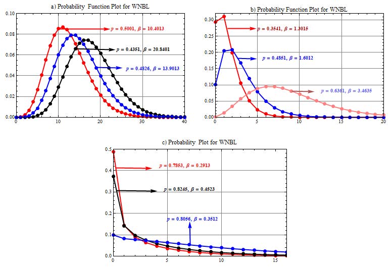
Figure 1 portrays that the WNBL distribution shows symmetrical behavior when p < 0.20 and β increases. Whereas, for smaller β and higher p, the distribution becomes positively skewed. The distribution also exhibits bimodal and reverse J shapes.

Now, we give two prime measures of the distribution.

The survival and hazard rate functions of the WNBL distribution are

$S_k=\frac{(1-p{)}^{\beta +1}{p}^k(\beta {)}_k}{(1+p({\beta }^2-1\left)\right)xk!}\times \left\{\right(1+\beta k){}_2{F}_1(\beta +k,1;k+1;p)+\frac{\beta p(\beta +k){}_2{F}_1(\beta +k+1,2;k+2;p)}{(k+1)}\}$ (4)

and

$h_k=\frac{(1+\beta k)(k+1)}{(1+\beta k)(k+1)\text{\_2F\_1}(\beta +k,1;k+1;p)+\beta p(\beta +k)\text{\_2F\_1}(\beta +k+1,2;k+2;p)},$ (5)

respectively. Where

$\text{\_2F\_1}(a,b;c;z)=\sum _{n=0}^{\infty }\frac{\left(a{)}_n\right(b{)}_n{z}^n}{(c{)}_{n}n!},$

and $(a{)}_n=a(a+1\left)\right(a+2\left)\dots \right(a+n-1)$, are the hypergeometric series function and the Pochhammer’s symbol, respectively, the series converges for $a,b,c\ge 0$ and $\left|z\right|\le 1$.

Clearly

$li{m}_{k\to \infty }{h}_k=(1-p{)}^2,$

therefore, the hazard rate function of the WNBL distribution is bounded above, which is an important property for the lifetime models.

Figure 2 displays increasing, decreasing and bathtub shape (BTS) hazard functions. It is observed that the traditional statistical distributions, such as the Poisson, generalized Poisson and NB distributions, cannot be used efficiently in models of count data with many zeros. The Poisson distribution tends to under-estimate the number of zeros, while the NB may over-estimate zeros (see Saengthong and Bodhisuwan 2013). Although the traditional count models have generally increasing or decreasing failure rates yet unable to exhibit BTS hazard rates.

Figure 2
Hazard Function Graphs for the Indicated Values of p and b of WNBL.

In view of the discussion above, some other motivational factors of the proposed model shall be outlined later and they are: i) Possessing BTS hazard function along with increasing/decreasing hazard rate characteristics which are seldom observed in discrete distributions. ii) Possessing bounded hazard function iii) Being an over- and under-dispersed statistical model. iv) Being a self decomposable and infinitely divisible model. v) Being a characterizable function which is a milestone in model selection.

STATISTICAL PROPERTIES OF THE WNBL DISTRIBUTION

The recognition of any discrete probability distribution is usually based on its probability generating function (pgf). The following theorem gives the pgf of the WNBL distribution.

Proposittion1: If $Y\sim$ WNBL $(p,\beta ),$ then the pgf of the random variable Y is expressed as

$G_Y\left(t\right)=\frac{(1+pt({\beta }^2-1\left)\right)q^{\beta +1}}{(1+p({\beta }^2-1\left)\right)(1-pt{)}^{\beta +1}},$ (6)

where$p\in (0,1)$ and $\beta \ge 0.$

Proof: The pgf from the definition is expressed as $G_Y\left(t\right)={\sum }_{x=0}^{\infty }{t}^{x}P(Y=x)$. Using equation (3), we have

$G_Y\left(t\right)=\frac{q^{\beta +1}}{1+p({\beta }^2-1)}\underset{x=0}{\overset{\infty }{\sum }}(\frac{\beta +x-1}{x})\left(pt{)}^x\right(1+\beta x)$

which by simplification, equation (6) is obtained, which completes the proof.

Corollary 1: In equation (6), if t is replaced by e^t, we get the moment generating function (mgf) of the WNBL distribution as

$M_Y\left(t\right)=\frac{(1+p{e}^t({\beta }^2-1\left)\right)q^{\beta +1}}{(1+p({\beta }^2-1\left)\right)(1-p{e}^t{)}^{\beta +1}},$ (7)

where $0<p{e}^t<1$.

The r^th derivatives of equation (7) with respect to t at t = 0 yield the moments. In particular, for r = 1 we have

${\mu }_1^{\prime }=\frac{\beta p(1+\beta +p({\beta }^2-1\left)\right)}{(1-p)(1+p({\beta }^2-1\left)\right)},$

for r = 2 we have

${\mu }_2^{\prime }=\frac{\beta (1+\beta )p(1-p(1-3\beta -(\beta -1)\beta p\left)\right)}{(1-p{)}^2(1+p({\beta }^2-1))},$

for r = 3 we have

${\mu }_3^{\prime }=\frac{\beta (1+\beta )p(1+p(-p+\beta (7+p(-1+6\beta +(-1+\beta )\beta p\left)\right)\left)\right)}{(1-p{)}^3(1+p({\beta }^2-1))}$

and for r = 4 we have

$\begin{array}{ccc}\hfill {\mu }_4^{\prime }& =\hfill & \hfill \frac{1}{(1-p{)}^4(1+p({\beta }^2-1))}\times \\ \hfill & \hfill & \hfill \left\{\beta \right(1+\beta \left)p\right(1+p(3+15\beta +(-3+\beta (11+25\beta ))p\\ \hfill & \hfill & \hfill +(-1+\beta (-2+\beta +10{\beta }^2\left)\right)p^2+(-1+\beta ){\beta }^3{p}^3\left)\right)\}.\end{array}$

Moreover, by definition, the r^th non central moment can be expressed as

${\mu }_r^{\prime }=\frac{(1-p{)}^{\beta +1}}{1+p({\beta }^2-1)}\sum _{x=0}^{\infty }{x}^r\left(\frac{\beta +x-1}{x}\right)(1+\beta x)p^x.$

Differentiating the equation above with respect to p we get

$\begin{array}{ccc}\hfill \frac{d{\mu }_r^{\prime }}{dp}& =\hfill & \hfill -\sum _{x=0}^{\infty }{x}^r\left(\frac{\beta +x-1}{x}\right)(1+\beta x)p^x\{\frac{({\beta }^2-1)(1-p{)}^{\beta +1}}{(1+p({\beta }^2-1){)}^2}+\frac{(\beta +1)(1-p{)}^{\beta }}{(1+p({\beta }^2-1\left)\right)}\}\\ \hfill & \hfill & \hfill +\frac{(1-p{)}^{\beta +1}}{1+p({\beta }^2-1)}\sum _{x=0}^{\infty }{x}^{r+1}\left(\frac{\beta +x-1}{x}\right)(1+\beta x)p^{x-1},\end{array}$

which by simplification yields the recurrence relation

${\mu }_{r+1}^{\prime }=p\frac{d{\mu }_r^{\prime }}{dp}+\frac{p(\beta +1)\left(\right(\beta -1\left)\right(1-p)+1+p({\beta }^2-1\left)\right)}{(1-p)(1+p({\beta }^2-1){)}^2}{\mu }_r^{\prime },$

$r=0,1,\dots ,$${\mu }_0^{\prime }=1$.

Similarly, by definition, the r^th central moment can be expressed as

${\mu }_r=\frac{(1-p{)}^{\beta +1}}{1+p({\beta }^2-1)}\sum _{x=0}^{\infty }(x-\frac{\beta p(1+\beta +p({\beta }^2-1\left)\right)}{(1-p)(1+p({\beta }^2-1\left)\right)}{)}^r\left(\frac{\beta +x-1}{x}\right)(1+\beta x)p^x.$

Differentiating the above equation with respect to p and simplifying it, we get

${\mu }_{r+1}+{\mu }_1^{\prime }{\mu }_r=p\frac{d{\mu }_r}{dp}+\frac{p\beta (\beta +1)(1-p{)}^{\beta }(1+p(\beta -1))}{(1+p({\beta }^2-1){)}^2}{\mu }_r+\frac{r(\beta +1)\left(\right(1+p({\beta }^2-1){)}^2+(\beta -1)(1-p{)}^2)}{(1-p{)}^2(1+p({\beta }^2-1){)}^2}{\mu }_{r-1}$

$r=1,2,\dots ,{\mu }_0^{\prime }=1$.

OVER-AND UNDER-DISPERSION

In statistics, the phenomenon of over- and under-dispersion relative to the Poisson distribution is generally observed in count data and well known in statistical literature. There are various causes of such phenomenon, like heterogeneity and aggregation for over-dispersion and repulsion for under-dispersion although less frequent (see Kokonendji and Mizre 2005). In order to see the reflection of over- and under-dispersion pattern, the researchers usually take the support of the index of dispersion (ID) which is defined as variance-to-mean ratio, which indicates the suitability of distribution in, under- or over-dispersed data sets. If $ID>1(<1)$ the distribution is over-dispersed (under-dispersed). The index of dispersion for the WNBL distribution is

$ID=\frac{1}{1-p}-\frac{1}{1-p+\beta p}+\frac{1}{1+p({\beta }^2-1)}.$

For indicating the dispersion pattern we first consider that β < 1 which implies that ${\beta }^2-1\le \beta -1$. If ${\beta }^2-1=-C$ and $\beta -1=-D$ then ID can be re expressed as

$ID=\frac{1}{1-p}-\frac{1}{1-pD}+\frac{1}{1-pC},$

since C > D then 1- pC < 1-pD or $\frac{1}{1-pC}-\frac{1}{1-pD}>0$. Therefore, the WNBL is an over-dispersed model for all values of p. However, if β >1 this implies that ${\beta }^2-1>\beta -1$. Let ${\beta }^2-1=L$ and $\beta -1=S,$ then ID can be rewritten as

$ID=\frac{1}{1-p}-\frac{1}{1+pS}+\frac{1}{1+pL}.$

As it is evident that L > S, then $\frac{1}{1+pL}<\frac{1}{1+pS}$ or $0<\frac{1}{1+pS}-\frac{1}{1+pL}<1$. Hence, ID< 1 if $p\to 0$ and $\beta \to \infty$.

OTHER MOMENTS MEASURES

The following theorems gives factorial moments and negative moments.

Theorem 1: If $Y\sim$ WNBL$(p,\beta )$, then the r^th descending factorial moment of Y is given by

${\mu }_{\left(r\right)}^{\prime }=\frac{\left(\beta {)}_r{p}^r\right(1-p{)}^{-r}(1+\beta r+({\beta }^2-1\left)p\right)}{(1+p({\beta }^2-1\left)\right)},$ (8)

where $p\in (0,1),$ $\beta \ge 0,$ $r=0,1,\dots ,(a{)}_n=a(a+1\left)\right(a+2\left)\dots \right(a+n-1)$ and ${\mu }_{\left(0\right)}^{\prime }=1$.

Proof: The r^th descending factorial moment for Y can be defined as ${\mu }_{\left(r\right)}^{\prime }=E\left(Y^{\left(r\right)}\right)={\sum }_{x=0}^{\infty }{x}^{\left(r\right)}P(Y=x)$. Using the expression $x^{\left(r\right)}=x(x-1)\dots (x-r+1)=\frac{x!}{(x-r)!}$, we have

${\mu }_{\left(r\right)}^{\prime }=\frac{(1-p{)}^{\beta +1}}{(1+p({\beta }^2-1\left)\right)}\sum _{x=r}^{\infty }\frac{x!}{(x-r)!}\left(\frac{\beta +x-1}{x}\right)(1+\beta x)p^x.$

By using the binomial series $(1-z{)}^{-a}=\underset{x=0}{\overset{\infty }{\sum }}\frac{(a{)}_n{z}^n}{n!}$, we obtain

${\mu }_{\left(r\right)}^{\prime }=\frac{(1-p{)}^{\beta +1}(\beta +r-1)!p^r}{(\beta -1)!(1+p({\beta }^2-1\left)\right)}\left\{\right(1-p{)}^{-(\beta +r)}+\beta (r+(r+1\left)\right(\beta +r)p+(\beta +r{)}_2(r+2)\frac{p^2}{2!}\dots \left)\right\},$

hence, we get

${\mu }_{\left(r\right)}^{\prime }=\frac{(1-p{)}^{-r}(\beta +r-1)!p^r}{(\beta -1)!(1+p({\beta }^2-1\left)\right)}\left\{\right(1-p{)}^{-(\beta +r)}+(1-p{)}^{-(\beta +r+1)}\beta (r+\beta p\left)\right\}.$

After some algebraic manipulation, the equation (8) is attained and it generates a recursive relation between r and (r - 1) descending factorial moments as

${\mu }_{\left(r\right)}^{\prime }\left\{\right(1-p\left)\right(1+\beta (r-1)+({\beta }^2-1)p\left)\right\}=\left\{\right(\beta +r-1\left)p\right(1+\beta r+({\beta }^2-1)p\left)\right\}{\mu }_{(r-1)}^{\prime },$ (9)

where $r=1,2,\dots ,$which completes the proof.

Theorem 2: If $Y\sim$ WNBL $(p,\beta )$, the r^th ascending factorial moment of Y is given by

${\mu }_{\left[r\right]}^{\prime }=\frac{\beta pr!(1-p{)}^{\beta +1}}{(1+p({\beta }^2-1\left)\right)}\{\text{\_2F\_1}(r+1,\beta +1;2;p)+\beta \text{\_2F\_1}(r+1,\beta +1;1;p)\},$ (10)

where $p\in (0,1),$ $\beta \ge 0,$ $r=0,1,...,$ ${\mu }_{\left[0\right]}^{\prime }=1-\frac{(1-p{)}^{\beta +1}}{(1+p({\beta }^2-1\left)\right)}$.

Proof: The r^th ascending factorial moment is defined as ${\mu }_{\left[r\right]}^{\prime }=E\left(\right(Y{)}_r)={\sum }_{x=0}^{\infty }(x{)}_{r}P(Y=x)$, this implies that

${\mu }_{\left[r\right]}^{\prime }=\frac{(1-p{)}^{\beta +1}}{(1+p({\beta }^2-1\left)\right)}\left\{\sum _{x=0}^{\infty }\left(\frac{\beta +x-1}{x}\right)\right(x{)}_r{p}^x+\beta \sum _{x=0}^{\infty }\left(\frac{\beta +x-1}{x}\right)x\left(x{)}_r{p}^x\right\}.$

By using the hypergeometric series function $\text{\_2F\_1}(a,b;c;z)={\sum }_{n=0}^{\infty }\frac{\left(a{)}_n\right(b{)}_n{z}^n}{(c{)}_{n}n!}$, we get the equation (10), where

$\underset{x=0}{\overset{\infty }{\sum }}(\frac{\beta +x-1}{x})(x{)}_r{p}^x=\beta r!p{}_2{F}_1(r+1,\beta +1;2;p)$

and

$\beta \underset{x=0}{\overset{\infty }{\sum }}(\frac{\beta +x-1}{x})x(x{)}_r{p}^x={\beta }^{2}r!p{}_2{F}_1(r+1,\beta +1;1;p)$

Thus the theorem is proved.

As it is known, the ordinary moments are generally helpful in estimating the unknown parameters. However, due to recent developments in inverse theory of the random variables, the negative moments are gaining momentum in life testing phenomena, estimation purposes and identifying the models. The negative moments are being used in irreversible damage to manufacturing materials due to damage process such as creep, corrosion, creep fracture, wear, shrinkage, aging and cracking (see Ahmad 2007). Therefore, the next theorem deals with the negative moments of the WNBL distribution.

Theorem 3: If $Y\sim$ WNBL$(p,\beta ),$ the first order negative moment of Y is given by

$E\left(\right(Y+a{)}^{-1})=\frac{(1-p{)}^{\beta +1}}{(1+p({\beta }^2-1\left)\right)}\{\frac{1}{a}{}_2{F}_1(a,\beta ;a+1;p)+\frac{{\beta }^{2}p}{a+1}{}_2{F}_1(a+1,\beta +1;a+2;p)\}$ (11)

where $p\in (0,1),$ $\beta \ge 0,$ $a>0$ and $\text{\_2F\_1}(a,b;c;z)={\sum }_{n=0}^{\infty }\frac{\left(a{)}_n\right(b{)}_n{z}^n}{(c{)}_{n}n!}$.

Proof: By definition, $E\left(\frac{1}{Y+a}\right)={\sum }_{x=0}^{\infty }\frac{P(Y=x)}{x+a}$, we have

$E\left(\frac{1}{Y+a}\right)=\frac{(1-p{)}^{\beta +1}}{(1+p({\beta }^2-1\left)\right)}\sum _{x=0}^{\infty }\left(\frac{\beta +x-1}{x}\right)(x+a{)}^{-1}{p}^x(1+\beta x).$

By simplification, we get the equation (11) where

$\sum _{x=0}^{\infty }\left(\frac{\beta +x-1}{x}\right)\frac{p^x}{x+a}=\frac{1}{a}\text{\_2F\_1}(a,\beta ;a+1;p)$

and

$\underset{x=0}{\overset{\infty }{\sum }}(\frac{\beta +x-1}{x})\frac{x{p}^x}{x+a}=\frac{\beta p}{(a+1)}{}_2{F}_1(a+1,\beta +1;a+2;p)$

This completes the proof.

Corollary 2: The r^th order negative moment of $Y\sim$ WNBL$(p,\beta )$ can be expressed as

$\begin{array}{ccc}\hfill E\left(\right(Y+a{)}^{-s})& =\hfill & \hfill \frac{(1-p{)}^{\beta +1}}{(1+p({\beta }^2-1\left)\right)}\left\{\frac{1}{a^s}{}_{s+1}\text{F}{}_s\right(a,...,a,\beta ;a+1,...,a+1;p)\\ \hfill & \hfill & \hfill +\frac{{\beta }^{2}p}{(a+1{)}^s}{}_{s+1}\text{F}{}_s(a+1,...,a+1,\beta +1;a+2,...,a+2;p)\},\end{array}$

where

${}_s\text{F}{}_u(a_1,...,a_s;b_1,...,b_u;z)=\sum _{n=0}^{\infty }\frac{(a_1{)}_n,...,(a_s{)}_n{z}^n}{(b_1{)}_n,...,(b_u{)}_{n}n!},$

the series converges for $s=u+1$ and $\left|z\right|<1$.

PARAMETER ESTIMATION AND INFERENCE

In this section, estimation of parameters of the distribution is investigated by the methods of moments (MM) and maximum likelihood (ML), and a performance of the estimators is assessed by a simulation study.

MOMENTS METHOD

Let $Y_1,Y_2,\dots ,Y_n$ be a random sample drawn from the WNBL distribution with the observed values $x_1,x_2,\dots ,x_n$. Equating the first two sample moments, $m_1^{\prime }=\bar{x}=\frac{1}{n}{\sum }_{i=1}^n{x}_i$ and $m_2^{\prime }=\frac{1}{n}{\sum }_{i=1}^n{x}_i^2,$ with their associated population moments

${\mu }_1^{\prime }=\frac{(\beta +1)p}{1-p}+\frac{({\beta }^2-1)p}{1+p({\beta }^2-1)}$

and

${\mu }_2^{\prime }={\mu }_1^{\prime }+\frac{\left(\right(\beta +1\left)\right(\beta +2\left)p^2\right)}{(1-p{)}^2}+\frac{2(\beta +1)({\beta }^2-1)p^2}{(1-p)(1+p({\beta }^2-1\left)\right)}$

then the MM estimators of the WNBL are obtained.

Alternatively, the MM estimators can also be obtained using the suggested approach by Khan et al. (1989) via minimizing the expression

$𝔖=({\mu }_1^{\prime }-m_1^{\prime }{)}^2+({\mu }_2^{\prime }-m_2^{\prime }{)}^2,$

with respect to p and β. Hence,

$S=(\frac{(\beta +1)p}{1-p}+\frac{({\beta }^2-1)p}{1+p({\beta }^2-1)}-m_1^{\prime }{)}^2+(m_1^{\prime }+\frac{\left(\right(\beta +1\left)\right(\beta +2\left)p^2\right)}{(1-p{)}^2}+\frac{2(\beta +1)({\beta }^2-1)p^2}{(1-p)(1+p({\beta }^2-1\left)\right)}-m_2^{\prime }{)}^2$

yields two equations which are not in closed form, so parameters are estimated using numerical optimization techniques via Mathematica 8 computational packages.

MAXIMUM LIKELIHOOD METHOD

If $Y_1,Y_2,\dots ,Y_n$ is a random sample drawn from the WNBL distribution with the observed values $x_1,x_2,\dots ,x_n,$ then we get the log-likelihood function

$\begin{array}{ccc}\hfill {\kappa }_{p,\beta }& =\hfill & \hfill ln\left(L\right(p;\beta \left)\right)=(\beta +1)nln(1-p)-nln\left(\right(1+p({\beta }^2-1)\left)\right)+\sum _{i=1}^n{x}_{i}lnp\\ \hfill & \hfill & \hfill +\sum _{i=1}^{n}ln\left(\frac{\beta +x_i-1}{x_i}\right)+\sum _{i=1}^{n}ln(1+\beta x_i).\end{array}$

By partially differentiating both sides of the equation above with respect to p and β and equating them to zero, we get the MLEs of pand β respectively, as

$\frac{n(\beta +1)}{1-p}+\frac{n({\beta }^2-1)}{1+p({\beta }^2-1)}=\frac{\bar{x}}{p}$ (12)

and

$nln(1-p)-\frac{2np\beta }{1+p({\beta }^2-1)}+\underset{i=1}{\overset{n}{\sum }}\frac{x_i}{1+\beta x_i}+\underset{i=1}{\overset{n}{\sum }}\left\{{\psi }^{\left(0\right)}\right(\beta +x_i)-{\psi }^{\left(0\right)}(\beta \left)\right\}=0$ (13)

Similarly, the second derivatives of the equation (12)) and equation (13) with respect to p and β, respectively, are

$\frac{{\partial }^2{\kappa }_{p,\beta }}{\partial p^2}=-\frac{n(\beta +1)}{(1-p{)}^2}+\frac{n({\beta }^2-1{)}^2}{1+p({\beta }^2-1)}-\frac{\underset{i=1}{\overset{n}{\sum }}{x}_i}{p^2}$

and

$\frac{{\partial }^2{\kappa }_{p,\beta }}{\partial {\beta }^2}=\frac{4n{p}^2{\beta }^2}{(1+p({\beta }^2-1){)}^2}-\underset{i=1}{\overset{n}{\sum }}\frac{x_i^2}{(1+\beta x_i{)}^2}-\frac{2np}{1+p({\beta }^2-1)}+\underset{i=1}{\overset{n}{\sum }}\left\{{\psi }^{\left(1\right)}\right(\beta +x_i)-{\psi }^{\left(1\right)}(\beta \left)\right\}$

Also, the second derivative of equation (12) with respect to β or equation (13) with respect to p yields

$\frac{{\partial }^2{\kappa }_{p,\beta }}{\partial \beta \partial p}=\frac{2\beta ({\beta }^2-1)np}{(1+p({\beta }^2-1){)}^2}-\frac{n}{1-p}-\frac{\beta n}{1+p({\beta }^2-1)},$

where ${\psi }^{\left(n\right)}\left(z\right)=\frac{d^n\psi \left(z\right)}{d{z}^n}$ is the logarithmic derivative of the gamma function. The MLEs are computed using computational packages, such as Mathematica 7. In view of the regularity conditions (see Rohatgi and Saleh 2002, pp. 419), we observed that the MLEs of WNBL parameters satisfy such conditions, where i) The parameters $p\in (0,1),\beta \in (0,\infty )$ are subset of the real line, ii)$\frac{\partial {\kappa }_{p,\beta }}{\partial p},\frac{\partial {\kappa }_{p,\beta }}{\partial \beta },\frac{{\partial }^2{\kappa }_{p,\beta }}{\partial p^2},\frac{{\partial }^2{\kappa }_{p,\beta }}{\partial {\beta }^2},\frac{{\partial }^2{\kappa }_{p,\beta }}{\partial p\partial \beta }$ exist for all values of p and β, iii) $E\left(\frac{\partial {\kappa }_{p,\beta }}{\partial p}\right)=0,E\left(\frac{\partial {\kappa }_{p,\beta }}{\partial \beta }\right)=0,$ iv) $\infty \le E\left(\frac{{\partial }^2{\kappa }_{p,\beta }}{\partial p^2}\right)\le 0,-\infty \le E\left(\frac{{\partial }^2{\kappa }_{p,\beta }}{\partial {\beta }^2}\right)\le 0$ for all values of p and β.

Moreover, the MLEs $\hat{p}$ and $\hat{\beta }$ of the WNBL distribution have an asymptotic bivariate normal distribution with vector mean (p,β) and variance-covariance matrix (I(p,β))^-1, where I(p,β) denotes the information matrix given by

$I\left(\right(p,\beta \left){|}_{p=\hat{p},\beta =\hat{\beta }}\right)=\left[\begin{array}{cc}\hfill 𝔼\left(\frac{-{\partial }^2{\kappa }_{p,\beta }}{\partial p^2}\right)\hfill & \hfill 𝔼\left(\frac{-{\partial }^2{\kappa }_{p,\beta }}{\partial p\partial \beta }\right)\hfill \\ \hfill 𝔼\left(\frac{-{\partial }^2{\kappa }_{p,\beta }}{\partial p\partial \beta }\right)\hfill & \hfill 𝔼\left(\frac{-{\partial }^2{\kappa }_{p,\beta }}{\partial {\beta }^2}\right)\hfill \end{array}\right]$,

where

$𝔼\left(\frac{-{\partial }^2{\kappa }_{p,\beta }}{\partial p^2}\right)=\frac{n(\hat{\beta }+1)}{(1-\hat{p}{)}^2}-\frac{n({\hat{\beta }}^2-1{)}^2}{1+\hat{p}({\hat{\beta }}^2-1)}+\frac{n𝔼\left(Y\right)}{{\hat{p}}^2},$

$𝔼\left(\frac{-{\partial }^2{\kappa }_{p,\beta }}{\partial p\partial \beta }\right)=-\frac{2\hat{\beta }({\hat{\beta }}^2-1)n\hat{p}}{(1+\hat{p}({\hat{\beta }}^2-1){)}^2}+\frac{n}{1-\hat{p}}-\frac{2\hat{\beta }n}{1+\hat{p}({\hat{\beta }}^2-1)},$

$𝔼\left(\frac{-{\partial }^2{\kappa }_{p,\beta }}{\partial {\beta }^2}\right)=-\frac{4n{\hat{p}}^2{\hat{\beta }}^2}{(1+\hat{p}({\hat{\beta }}^2-1){)}^2}+n𝔼\left(\frac{Y^2}{(1+\hat{\beta }Y{)}^2}\right)+\frac{2n\hat{p}}{1+\hat{p}({\hat{\beta }}^2-1)}-n𝔼\left\{{\psi }^{\left(1\right)}\right(\hat{\beta }+Y)-{\psi }^{\left(1\right)}(\hat{\beta }\left)\right\}.$

The expectations above can be obtained numerically.

SIMULATION SCHEME

As it is mentioned in the introduction that the WNBL(p,β) distribution can be viewed as a mixture of the negative binomial, NB(p,β), and size biased negative binomial, SBNB(p,β), distributions. So, in order to generate random data k_i, i=1,2,...n, from the WNBL we used the following algorithm.

Algorithm: i) Generate U_i,i = 1,2,...,n,from the uniform distribution on the interval (o,1). ii) Generate NB_i,i=1,2,...,n from the negative binomial distribution NB(p,β) with support k=0,1,.... iii)Set Y₁=NB_i. iv) Generate SBNB_i,i=1,2,...,n, from the size biased negative binomial distribution SBNB(p,β) with support k=1,2,.... v) Set Y₂=SBNB_i. If $U_i\le \frac{1-p}{(1+p({\beta }^2-1\left)\right)}$, then set k_i=Y₁ otherwise set k_i=Y₂,i=1,2,...,n.

SIMULATION STUDY

In this section, we perform some numerical experiments to see how the estimates studied by using the above listed methods (MM and ML) as well as their asymptotic results for finite samples. All the numerical results are performed via Mathematica 8 using the random numbers generator code. We consider the following different model parameters. Model-I: $\beta =0.0542,p=0.7487$, Model-II: $\beta =30.4389,p=0.0157$ and Model-III: $\beta =5.2856,p=0.6398$ for both MMEs and MLEs. We consider the following sample sizes n=20(small), 50 (moderate), and 100,200,500 (large). For each set of the model parameters and for each sample size, we compute the MMEs and MLEs of each β and p. We repeat this process 1000 times and compute the average bias and mean square error (MSE) for all replications in the relevant sample sizes. The results are reported in Table I and III.

Discussion: Some notes are very clear from the simulation studies, such as the bias decreases as sample size increases for both MLEs and MMEs. Moreover, we conclude that the bias takes negative and positive signs, and it approaches to the value zero for both signs while the MSE decreases as the sample size increases.

TABLE I
Average Bias and MSE values of the MMEs from simulation of the WNBL distribution.

Parameter	Sample Size	Bias($\hat{\beta }$)	Bias($\hat{p}$)	MSE($\hat{\beta }$)	MSE($\hat{p}$)
β = 0:0542, p = 0:7487	n=20	26.6700	-0.7485	742.1	0.5603
	n=50	14.5694	-0.6458	411.023	0.4276
	n=100	1.1141	-0.6022	1.4983	0.4265
	n=200	0.9135	-0.5743	0.9130	0.3924
	n=500	0.8783	-0.5517	0.8940	0.3822
β = 30:4389, p = 0:0157	n=20	139.4975	-0.7418	37071.8	0.5502
	n=50	4.7926	-0.7071	23.0087	0.5001
	n=100	4.4596	-0.6744	19.4900	0.4995
	n=200	3.8780	-0.6688	18.8034	0.4872
	n=500	2.8913	-0.6217	15.8204	0.4644
β= 5:2856, p = 0:6398	n=20	4.0410	-0.0942	12.6543	0.0125
	n=50	3.6904	-0.0907	12.1628	0.0063
	n=100	3.6522	-0.0890	9.8270	0.0058
	n=200	3.3172	-0.0836	8.5084	0.0056
	n=500	2.6516	-0.0798	8.2922	0.0047

TABLE II
Average Bias and MSE values of the MLEs from simulation of the WNBL distribution.

Parameter	Sample Size	Bias($\hat{\beta }$)	Bias($\hat{p}$)	MSE($\hat{\beta }$)	MSE($\hat{p}$)
β = 0:0542, p = 0:7487	n=20	32.0968	-0.7486	1030.22	0.5604
	n=50	14.498	-0.6101	410.9645	0.3914
	n=100	0.9708	-0.5826	1.1641	0.3570
	n=200	0.7625	-0.5720	0.6627	0.3545
	n=500	0.6575	-0.5606	0.6321	0.3532
β = 30:4389, p = 0:0157	n=20	138.775	-0.7417	36685.5	0.5502
	n=50	4.1503	-0.6758	18.827	0.4968
	n=100	3.6311	-0.6408	17.574	0.4888
	n=200	3.3901	-0.6212	16.8538	0.4837
	n=500	2.3361	-0.5537	14.3888	0.4327
β = 5:2856, p = 0:6398	n=20	3.3960	-0.0869	11.5333	0.0075
	n=50	3.0078	-0.0866	11.3053	0.0055
	n=100	2.5571	-0.0866	10.3211	0.0052
	n=200	2.4807	-0.0752	7.7243	0.0045
	n=500	1.6978	-0.0728	5.1232	0.0042

CHARACTERIZATION

Characterization of probability functions is of importance to determine the exact probability distribution, which means that under certain conditions a family of distributions is the only one possessing a designated property which will resolve the problem of model identification. Therefore, the next theorem gives characterization of the WNBL distribution.

Theorem 4: If $G_Y\left(t\right)={\sum }_{x=0}^{\infty }{x}^{t}P(Y=x)$ is the pgf of a certain distribution defined on the support $\{0,1,2,\dots \}$ with parameters $p\in (0,1),$ $\beta \ge 0$, then

${\mu }_{\left(r\right)}^{\prime }\left\{\right(1-p\left)\right(1+\beta (r-1)+({\beta }^2-1)p\left)\right\}=\left\{\right(\beta +r-1\left)p\right(1+\beta r+({\beta }^2-1)p\left)\right\}{\mu }_{(r-1)}^{\prime },$ (14)

for $r=1,2,\dots$ with ${\mu }_{\left(0\right)}^{{}^{\prime }}=1$, holds if and only if Y has the WNBL distribution with pmf defined by equation (3).

Proof: If $Y$ has the WNBL distribution given by (3), then the equation (14)) is satisfied.

On the other side, suppose the equation (9) holds, which yields descending factorial moments, hence for $r=1$ and ${\mu }_{\left(0\right)}^{{}^{\prime }}=1,$ we have

${\mu }_{\left(1\right)}^{\prime }=\frac{\left(\beta \right)p(1-p{)}^{-1}(1+\beta +({\beta }^2-1)p)}{(1+p({\beta }^2-1\left)\right)}.$

For r=2 and ${\mu }_{\left(1\right)}^{{}^{\prime }}$ expressed in the above equation, we get

${\mu }_{\left(2\right)}^{\prime }=\frac{\left(\beta {)}_2{p}^2\right(1-p{)}^{-2}(1+2\beta +({\beta }^2-1\left)p\right)}{(1+p({\beta }^2-1\left)\right)}.$

Also, for r=3 and ${\mu }_{\left(2\right)}^{{}^{\prime }}$ expressed in the equation above, we obtain

${\mu }_{\left(3\right)}^{\prime }=\frac{\left(\beta {)}_3{p}^3\right(1-p{)}^{-3}(1+3\beta +({\beta }^2-1\left)p\right)}{(1+p({\beta }^2-1\left)\right)},$

and so on. Since, factorial moment generating function is defined as

$G_Y(1+t)=\sum _{r=0}^{\infty }{\mu }_{\left(r\right)}^{\prime }\frac{t^r}{r!},$ (15)

by substituting ${\mu }_{\left(0\right)}^{\prime },{\mu }_{\left(1\right)}^{\prime },{\mu }_{\left(2\right)}^{\prime },{\mu }_{\left(3\right)}^{\prime }$ and so on in equation (15) we get

$G_Y(1+t)=1+\frac{\beta pt}{(1-p)1!}+\frac{{\beta }^{2}pt}{(1-p)(1+p({\beta }^2-1\left)\right)1!}+\frac{\beta (\beta +1)p^2{t}^2}{(1-p{)}^{2}2!}+\frac{{\beta }^2(\beta +1)p^2{t}^2}{(1-p{)}^2(1+p({\beta }^2-1))2!}+\frac{\beta (\beta +1)(\beta +2)p^3{t}^3}{(1-p{)}^{3}3!}+\frac{{\beta }^2(\beta +1)(\beta +2)p^3{t}^3}{(1-p{)}^3(1+p({\beta }^2-1))3!}+\dots .$

Hence,

$G_Y(1+t)=1+\frac{\beta pt}{(1-p)1!}+\frac{(\beta {)}_2{p}^2{t}^2}{(1-p{)}^{2}2!}+\frac{(\beta {)}_3{p}^3{t}^3}{(1-p{)}^{3}3!}+\dots +\frac{{\beta }^{2}pt}{(1-p)(1+p({\beta }^2-1\left)\right)}\{1+\frac{(\beta +1)pt}{(1-p)1!}+\frac{(\beta +1{)}_2{p}^2{t}^2}{(1-p{)}^{2}2!}+\dots \}.$

After some algebra, we get

$G_Y(1+t)=\frac{(1-p{)}^{\beta +1}(1+p(1+t)({\beta }^2-1))}{(1-p(1+t\left){)}^{\beta +1}\right(1+p({\beta }^2-1))}.$

Replacing $(1+t)$ by t we have

$G_Y\left(t\right)=\frac{(1-p{)}^{\beta +1}(1+pt({\beta }^2-1))}{(1-pt{)}^{\beta +1}(1+p({\beta }^2-1))}.$

By calculating the x^th derivative of G_t(t) at t=0,

$P(Y=x)=\frac{\frac{{\partial }^x{G}_Y\left(t\right)}{\partial t^x}{|}_{t=0}}{x!},x=0,1,\dots ,$

yields equation (3). This completes the proof.

DISCRETE ANALOGUES OF SELF-DECOMPOSABILITY

Definition 5.1 (α-thinning) Let $X$ be a non-negative integer-valued random variable and let $\alpha \in [0,1]$ , then the α-thinning of X using the Steutel and van Harn operator is defined by

$\alpha \circ X:\equiv \sum _{i=1}^X{Z}_i,$

where Z_i(i=1,2,...,X) are mutually independent Bernoulli random variables with P(Z_i=1)= α and P(Z_i=0)=1-α. Additionally, the random variables Z_i are independent of X. The pgf $G_{\alpha \circ X}\left(s\right)$ of the random variable $\alpha \circ X$ is $G_{\alpha \circ X}\left(s\right)=G_X(1-\alpha +\alpha s).$

Definition 5.2 (Discrete Infinite divisibility) Let X be a non-negative integer-valued random variable, then X is said to be infinitely-divisible, for every non negative integer n, if X can be represented as a sum of n independent and identically distributed (i.i.d.) non-negative random variables X_n;i(i=1,2,...,n), that is,

$X\equiv X_{n,1}+X_{n,2}+...+X_{n,n},n=1,2,3,....$

Note that the distributions of X and X_n;i do not necessarily have to be of the same family. Moreover, a random variable X is said to be discrete infinitely-divisible if the random variables X_n;i only take non-negative integer values. A necessary condition for such random variable X to be well defined is P(X=0)>0 (to exclude the trivial case we assume P(X=0)<1), see Steutel and van Harn(1979).

Definition 5.3 (Discrete self-decomposability) A non-negative integer-valued random variable X is said to be discrete self-decomposable if for every $\alpha \in [0,1],$ the random variable X can be written as $X\equiv \alpha \circ X+X_{\alpha },$ where the random variables $\alpha \circ X$ and $X_{\alpha }$ are independent, which in terms of the pgf can be expressed as

$G_X\left(s\right)=G_X(1-\alpha +\alpha s)G_{X_{\alpha }}\left(s\right),$

where $G_{X_{\alpha }}\left(s\right)$ is the pgf of $X_{\alpha }$. We have noted that the distribution of $X_{\alpha }$ uniquely determines the distribution of X. Moreover, a discrete infinitely-divisible distribution is discrete self-decomposable.

By using the definitions above, the following propositions show that the WNBL distribution is a self decomposable and infinitely-divisible distribution.

Proposition 2: If X₁,X₂ and X₃ are independent random variables such that $X_1\sim$ Bernoulli$\left(\frac{p({\beta }^2-1)}{1+p({\beta }^2-1)}\right)$, $X_2\sim$NB(p,β) and $X_3\sim$Geo(1-p), then Y = X₁+ X₂+ X₃ has the WNBL(p,β) distribution.

Proof: Since $X_1\sim$ Bernoulli$\left(\frac{p({\beta }^2-1)}{1+p({\beta }^2-1)}\right)$, its mgf is expressed as $M_{X_1}\left(t\right)=\frac{1+p{e}^t({\beta }^2-1)}{1+p({\beta }^2-1)}$. Similarly, X₂ and X₃ having the mgfs $M_{X_2}\left(t\right)=\frac{(1-p{)}^{\beta }}{(1-p{e}^t{)}^{\beta }}$ and $M_{X_3}\left(t\right)=\frac{1-p}{1-p{e}^t},$ respectively. Since Y = X₁ + X₂ + X₃ hence the mgf of Y is

$M_Y\left(t\right)=\frac{1+p{e}^t({\beta }^2-1)}{1+p({\beta }^2-1)}\frac{(1-p{)}^{\beta }}{(1-p{e}^t{)}^{\beta }}\frac{1-p}{1-p{e}^t},$

which is the mgf of the WNBL distribution. This completes the proof.

Proposition 3: If $Y_i\sim$ WNBL $(p,\beta )$ for $i=1,2,...n$, are independent random variables, then $Z=Y_1+Y_2+Y_3\dots +Y_n$, and having the WNBL$(n,p,\beta )$ distribution.

Proof: As $Y_i\sim$ WNBL $(p,\beta )$ for $i=1,2,...n$, hence the mgf of $Z=$ $Y_1+Y_2+Y_3\dots +Y_n$ is

$M_Z\left(t\right)=\prod _{i=1}^n{M}_{Y_i}\left(t\right)=\frac{(1+p{e}^t({\beta }^2-1\left){)}^n\right(1-p{)}^{n(\beta +1)}}{(1+p({\beta }^2-1\left){)}^n\right(1-p{e}^t{)}^{n(\beta +1)}},$

which gives the required proof.

Note in the expression above

$M_Z\left(t\right)=M_{X_B}\left(t\right)M_{X_{NB}}\left(t\right),$

where $X_B\sim$ Binomial($\frac{p({\beta }^2-1)}{1+p({\beta }^2-1)},n$) and $X_{NB}\sim$ NB($p,n(\beta +1)$), which shows the discrete self-decomposability.

TEST STATISTICS WITH DATA APPLICATIONS

In this section, the credibility of the proposed model is checked via over- and under-dispersed count data sets. In this regard, for modeling over-dispersion phenomena, we have used three data sets: (i) The counts of European red mites on apple leaves, (ii) Accidents of 647 women working on H.E. shells during five weeks, (iii) The thunder storm activity at Cape Kennedy. While, for under-dispersion case the number of outbreaks of strikes in UK coal mining industries is used. All the data sets are modeled via the four probability models: WNBL, NB, Poisson (Poi) and Generalized Poisson (GP) distributions. Since NB distribution is the compounded mixture of gamma and Poisson distributions, so it is usually recommended for heterogeneity and over-dispersion, while the generalized Poisson distribution is a mixed and weighted version as well as a generalized form of Poisson distribution, therefore it is used to model over- and under-dispersed data sets. The probability functions of these models are given in the next table

For comparison purposes, we have used seven goodness-of-fit statistics. The computation of these statistics is based on the MLEs which are computed by using Mathematica 7 computational package. These statistics include Log-Likelihood (l), Akaike information criterion (AIC), Bayesian information criterion (BIC) and corrected Akaike information criterion (AICc), Kolmogrov Smirnov (KS) statistics and ${\chi }^2$ statistics with p-values. The formulae of such statistics are $AIC=-2l\left(\hat{\theta }\right)+2m,$ $BIC=-2l\left(\hat{\theta }\right)+m$ $ln\left(n\right),$ $AICc=AIC+\frac{2m(m+1)}{n-m-1},$ $KS=Max\{\frac{i}{g}-z_i,z_i-\frac{i-1}{g}\}$ and ${\chi }^2={\sum }_{i=1}^g\frac{(o_i-e_i{)}^2}{e_i}$, where m denotes the number of parameters, $l\left(\hat{\theta }\right)$ denotes the log-likelihood function evaluated at the MLEs, n denotes the number of observations in a sample,g denotes the number of classes and $o_i$, $e_i$ and $z_i$ denote the observed frequencies, expected frequencies and cumulative distribution function of the $i^{th}$ class, respectively.

Vuong Test: The chi-square approximation to the distribution of the likelihood ratio test statistic is valid only for testing restrictions on the parameters of a statistical model, i.e., ${𝐇}_0$ and ${𝐇}_1$ are nested hypotheses. With non-nested models, we cannot make use of likelihood ratio tests for model comparison. In this case, information criteria, like AIC and BIC as well as the Vuong test for non-nested models are useful. Vuong (1989) proposed a likelihood ratio-based statistic for testing the null hypothesis that the competing models are equally close to the true data generating process against the alternative that one model is closer. Let us consider two statistical models based on the probability mass functions $f_A(x;\xi )$ and $f_B(x;\zeta )$ posses equal number of parameters. Define the likelihood ratio statistic for the model $f_A(x;\xi )$ against $f_B(x;\zeta )$ as

$𝔏\Re (\widehat{{\xi }_n},\widehat{{\zeta }_n})=\sum _{g=1}^G{f}_{g}ln\left(\frac{f_A(x;\widehat{{\xi }_n})}{f_B(x;\widehat{{\zeta }_n})}\right),$

where $\widehat{{\xi }_n}$ and $\widehat{{\zeta }_n}$ are the maximum likelihood estimators in each model based on n number of observations(see Denuit et al. 2007), $f_g$ denotes the observed frequency of the $g^{th}$ class and $G$ total number of classes . If both models are strictly non-nested then under ${𝐇}_0$ we have the test statistics $Z=\frac{LR(\widehat{{\xi }_n},\widehat{{\zeta }_n})}{\sqrt{n}\widehat{{\omega }_n}}\sim N(0,1)$, where

$\widehat{{\omega }_n}=\frac{1}{G}\underset{g=1}{\overset{G}{\sum }}{\left(ln\frac{f_A(x_g;\widehat{{\xi }_n})}{f_B(x_g;\widehat{{\zeta }_n})}\right)}^2-{\left(\frac{1}{G}\underset{g=1}{\overset{G}{\sum }}ln\frac{f_A(x_g;\widehat{{\xi }_n})}{f_B(x_g;\widehat{{\zeta }_n})}\right)}^2.$

In order to select an appropriate model, we usually construct the following hypothesis

${𝐇}_0;𝔎𝔏\left(f_A\right(x;\xi \left)\right)=𝔎𝔏\left(f_B\right(x;\zeta \left)\right),$

against

${𝐇}_{1A};𝔎𝔏\left(f_A\right(x;\xi \left)\right)<𝔎𝔏\left(f_B\right(x;\zeta \left)\right),$

i.e., the model A is defined to be better than model B if model A’s $𝔎𝔏$ distance to the truth is smaller than that of model B, or ${𝐇}_{1B};𝔎𝔏\left(f_A\right(x;\xi \left)\right)>𝔎𝔏\left(f_B\right(x;\zeta \left)\right).$ That is, the model B is defined to be better than model A if model B’s $𝔎𝔏$ distance to the truth is smaller than that of model A, where $𝔎𝔏$ denotes the Kullback-Leibler distance measure, with corresponding critical values. The decision is as follows. i) Reject ${𝐇}_0$ when $𝐙>{𝐙}_{ϵ}$ in favor of A and $ii)$ Reject ${𝐇}_0$ when $𝐙<-{𝐙}_{ϵ}$ in favor of B, where $ϵ$ denotes the level of significance.

DESCRIPTION OF THE DATA SETS WITH THEIR FITTING

In biological research, researchers are often concerned with animals and plants counts for each of set of equal units space and time. Among these sets of counts, some counts may perhaps be well fitted by the Poisson distribution where the equi-dispersion phenomenon in the data is observed. But in discrete data sets the two other dispersion cases are also observed. The over-dispersion generally arises when the events or organisms are aggregated, clustered or clumped in time and space, while the under-dispersion is due to more regular positioning than that produced by a Poisson mechanism (see Ross and Preece 1985). So, in the coming data applications we have also used the Vuong test for selecting a model which possesses the same number of parameters at significance level 0.08, for this purpose we have compared the proposed model with the NB and GP, not with the Poisson distribution because the latter one is unsuitable for over- and under-dispersed data.

The counts of European red mites on apple leaves(Data I):Garman (1951) of the Connecticut Agricultural Experiment Station selected 25 leaves at random from each of six McIntosh trees in a single orchard receiving the same spray treatment and the number of adult females counted on each leaf. These observations given in Table III of the Appendix and were first recorded by Bliss and Fisher (1953), and later on were mentioned by Jain and Consul (1971). The summary statistics of these observations is provided in Table Iv as given in Appendix which clearly indicates the over-dispersed nature of the data. In order to fit the competing models to this data set we have used the MLE estimates. The summary of test statistics is provided in Table V which depicts that the proposed model is the most suitable choice of such data with least loss of information. Moreover, the selection of a suitable non-nested model is also checked via Vuong test. The Vuong test statistics values along with p-value for comparison between WNBL-GP and WNBL-NB are given as i)Z=-1.7548, p-value=0.0793 and ii)Z=-1.7512, p-value=0.0799 which clearly indicates the suitability of the proposed model by showing minimum p-value.

Accidents to 647 women working on H. E. shells during five weeks(Data II): Miss Broughton, Head Welfare Officer, and the various Welfare Supervisors were the first to provide this numerical data set to Industrial Fatigue Research Board in 1919 (see Greenwood and Woods, 1919). Later on Greenwood and Yule (1920) and Jain and Consul (1971) used it for analysis purpose. This data set is displayed at Table VI and its descriptive statistics are provided in Table VII which shows an over-dispersed behavior. The earlier mentioned test statistics indicate that the proposed model is the most suitable one according to all mentioned statistics with least loss of information behavior and the results are displayed in Table VIII as given in the Appendix. Furthermore, the Vuong test statistics values along with p-value for comparison between WNBL-GP and WNBL-NB are given as i)Z=11.4348,p-value=0.0001 and ii) Z=18.08284,p-value=0.0001 which clearly indicates that the proposed model is better than the competing models.

Number of outbreaks of strikes in UK coal mining industries in four successive week periods during 1948-1959(Data III): This data set is given by Table IX and was analyzed by Castillo and Perez-Casany (1998), noting that they reported it from Kendall (1961). Later on a number of authors, like Ridout and Besbeas (2004), Chakraborty and Chakravarty (2012) and Alamatsaz and Dey (2016), studied it. Table X as given in the Appendix displays the descriptive statistics of this data set and indicates that it is under-dispersed. Further, comparison among the competing distributions is provided in Table XI which indicates that the proposed model is also an ideal model for under-dispersed data by showing not only the least Chi-Square test statistics but also minimum AIC, BIC and AICc, thus depicting that the model is the least loss of information model for under-dispersed data set too. Also, Vuong test statistics with p-values for comparison between WNBL-GP and WNBL-NB are listed as i)𝐙 = 1.8540, p-value=0.0673 and ii)𝐙=4.4281, p-value=0.0001 which again indicates the suitability of the proposed model.

Thunderstorm Activity at Cape Kennedy(Data IV): One of the major problem that the meteorologists usually faced is the forecasting of afternoon convective thunderstorm activity at the Cape Kennedy Florida. Usually thunderstorms are of primary concern in the design of launch vehicles, in the planning of space missions, and in launch operations at Cape Kennedy because of high winds, lightning hazard, and extreme turbulence associated with this atmospheric phenomenon. In thunderstorm activity, the occurrence of successive thunderstorm events (THEs) is often dependent process meaning that the occurrence of THEs indicates that the atmosphere is unstable and the environmental conditions are favorable for the formation of further thunderstorm activity. For more details on THEs, see Falls et al. (1971). Data set of thunderstorm activity at Cape Kennedy is displayed in Table XII at the Appendix. As for thunderstorm activities the Poisson distribution is not a proper choice, hence the proposed model is compared with the NB and GP distributions based on the expected frequencies, $l$, AIC, ${\chi }^2$ and p-values. The expected frequencies along with the test statistics of this data set are provided in the Tables XIII, XIV and XV. Vuong test statistics with p-values are displayed in Table XVI and Table XVII as given in Appendix, which clearly indicate the supremacy behavior of the proposed model over the competing distributions, except in February GP is recommended.

CONCLUSIONS

A new discrete model, named weighted negative binomial Lindley distribution, is proposed and its various properties are obtained involving generating functions, moments, recurrence relations between moments, random number generation, characterization, self-decomposability and infinite divisibility. Further, some applications of the model are studied. It is found that model is not only mathematically amenable but also recommended for many types of over- and under-dispersed count data sets. Moreover, the proposed model is also recommended for modeling the thunderstorms data and may help the scientists for proper planning of space missions and in launch operations at different stations in the presence of thunderstorms activities.

ACKNOWLEGMENTS

The author express his thanks to Associate Editor of the mathematical sciences area and the two referees for careful reading of the paper and providing valuable comments. Special thanks to Professor Tassaddaq Kiani for his sincere help during the progress of this paper.

REFERENCES

• AHMAD M. 2007. On the theory of inversion. Int J Stat Sci 6: 43-53.
• ALAMATSAZ MH AND DEY S. 2016. Discrete generalized Rayleigh distribution. Pak J Stat 32(1): 1-20.
• BALAKRISHNAN N. 2014. Methods and Applications of Statistics in Clinical Trials: Planning, Analysis and Inferential Methods. J Wiley & Sons, Inc.
• BLISS CI AND FISHER RA. 1953. Fitting the negative binomial distribution to biological data. Biometrics 9(2): 176-200.
• CASTILLO I AND PEREZ-CASANY M. 1998. Weighted Poisson distributions for overdispersion and underdispersion situations. Ann Inst Statist Math 50: 567-585.
• CHAKRABORTY S AND CHAKRAVARTY D. 2012. Discrete gamma distributions: Properties and parameter estimations. Commun Statist Theor Meth 41: 3301-3324.
• DENUIT M, MARCHAL X, PITREBOIS S AND WALHIN JF. 2007. Actuarial Modelling of Claim Counts Risk Classification Credibility and Bonus-Malus Systems. John Wiley.
• FALLS L, WILLIFORD WO AND CARTER MC. 1971. Probability distributions for thunderstorm activity at Cape Kennedy, Florida. J Appl Meteorol 10: 97-104.
• FISHER RA. 1934. The effects of methods of ascertainment upon the estimation of frequencies. Ann Eugenic 6: 13-25.
• GARMAN P. 1951. Original data on European red mite on apple leaves. Technical report. Report. Connecticut.
• GREENWOOD M AND WOODS HM. 1919. The Incidence of Industrial Accidents upon Individuals with Special Reference to Multiple Accidents. Industrials Fatigue Research Board Report URL https://ia802705.us.archive.org/29/items/ncidenceofindus00grea/incidenceofindus00grea.pdf. Online Address.
  » https://ia802705.us.archive.org/29/items/ncidenceofindus00grea/incidenceofindus00grea.pdf.
• GREENWOOD M AND YULE GU. 1920. An inquiry into the nature of frequency distributions representative of multiple happenings with particular reference to the occurrence of multiple attacks of disease or of repeated accidents. J Roy Stat Soc 83: 255-279.
• HUSSAIN T, ASLAM M AND AHMAD M. 2016. A two parameter discrete Lindley distribution. Rev Colomb Estad 39: 45-61.
• JAIN GC AND CONSUL PC. 1971. A generalized negative binomial distribution. SIAM J Appl Math 21: 501-5013
• JAIN K, SINGLA N AND GUPTA RD. 2014. A weighted version of gamma distribution. Discus Math Prob Stat 34: 89-111.
• KENDALL MG. 1961. Natural law in social sciences. J R Stat Soc Ser A 124: 1-19.
• KHAN AMS, KHALIQUE A AND ABOUAMMOTH AM. 1989. On estimating parameters in a discrete Weibull distribution. IEEE T Reliab 38: 348-350.
• KOKONENDJI CC AND CASANY MP. 2012. A note on weighted count distributions. J Stat Theory Appl 11: 337-352.
• KOKONENDJI CC AND MIZRE D. 2005. Overdispersion and Underdispersion Characterization of Weighted Poisson Distribution (Technical Report No. 0523) France LMA. Technical report.
• NEEL JV AND SCHULL WJ. 1966. Human Heredity. Chicago: University of Chicago Press.
• PATIL GP. 1991. Encountered data, statistical ecology, environmental statistics, and weighted distribution methods. Environmetrics 2: 377-423.
• PATIL GP AND RAO CR. 1977. Weighted distributions: a survey of their application. In Krishnaiah PR (Ed.), Applications of Statistics, pp. 383-405. North Holland Publishing Company.
• PATILL GP, RAO CR AND RATNAPARKHI M. 1986. On discrete weighted distribution and their use in model choice for observed data. Commun Statisit Theory Math 15: 907-918.
• RAO CR. 1985. Weighted distributions arising out of methods of ascertainment. In Atkinson AC AND Fienberg SE (Eds.), A Celebration of Statistics Chapter 24. pp. 543-569. New York: Springer-Verlag.
• RIDOUT MS AND BESBEAS P. 2004. An empirical model for under dispersed count data. Statist Model 4: 77-89.
• ROHATGI VK AND SALEH AKE. 2002. An Introduction to probability and Statistics. Singapore: John Wiley and Sons (Asia) Pte Ltd.
• ROSS GJS AND PREECE DA. 1985. The negative binomial distribution. The Statistician 34: 323-336.
• SAENGTHONG P AND BODHISUWAN W. 2013. Negative binomial-crack (NB-CR) distribution. Int J Pure Appl Math 84: 213-230.
• SAKAMOTO CM. 1973. Application of the Poisson and negative binomial models to thunderstorm and hail days probabilities in Nevada. Monthly Weather Review 101: 350-355.
• STEUTEL FW AND VAN HARN K. 1979. Discrete analogues of self-decomposability and stability. Ann Prob 7: 893-899.
• VUONG QH. 1989. Likelihood ratio tests for model selection and non-nested hypotheses. Econometrica 57: 307-333.

APPENDIX

Table III
Counts of numbers of European red mites on apple leaves; data from Garman, 1951.

Count	0	1	2	3	4	5	6	7	Total
Observed frequency	70	38	17	10	9	3	2	1	150

Table IV
Summary Statistics of data-I.

Mean	Variance	ID	MDμ	Skewness	Kurtosis
1.1466	2.2736	1.9828	1.1445	1.5291	4.9528

TABLE V
Tests Summary for data set I.

Distribution	$\hat{p}$	$\hat{\beta }$	KS	- $l$	df	${\chi }^2$	p-value	AIC	BIC	AICc
WNBL($\hat{p}$,$\hat{\beta }$)	0.2087(0.0154)	0.4770(0.0436)	0.5951	222.3063	3	2.3842	0.497	448.6126	454.6339	445.6926
NB($\hat{p}$,$\hat{\beta }$)	0.5281(0.0275)	1.0245( 0.1051)	0.5979	222.4371	3	2.5147	0.473	448.8742	454.8955	445.9542
GP($\hat{p}$,$\hat{\beta }$)	0.3209(0.0551)	0.7786(0.0796)	0.6019	222.7452	3	2.9475	0.400	449.4904	455.5117	446.5704
Pois.($\hat{\beta }$)		1.1466(0.0874)	0.6408	242.8099	2	26.6513	0.000	487.6198	490.6304	485.6465

Table VI
Accidents to 647 women working on H. E. shells during 5 weeks.

Count	0	1	2	3	4	5 or more	Total
Observed frequency	447	132	42	21	3	2	647

Table VII
Summary Statistics of data-II.

Mean	Variance	ID	MDμ	Skewness	Kurtosis
0.4652	0.6919	1.4872	0.6428	2.1212	7.9209

TABLE VIII
Tests Summary for data set II.

Distribution	$\hat{p}$	$\hat{\beta }$	KS	- $l$	df	${\chi }^2$	p-value	AIC	BIC	AICc
WNBL($\hat{p}$,$\hat{\beta }$)	0.3006(0.0140)	0.6160(0.0314)	0.7295	592.0683	2	2.9852	0.225	1188.137	1197.081	1185.155
NB($\hat{p}$,$\hat{\beta }$)	0.3497(0.0137)	0.8651(0.0587)	0.7309	592.2670	2	3.2742	0.195	1188.534	1197.479	1185.553
GP($\hat{p}$,$\hat{\beta }$)	0.1963(0.0332)	0.3739(0.0253)	0.7328	592.6005	2	3.7961	0.150	1189.201	1198.146	1186.22
Pois.($\hat{\beta }$)		0.4652(0.0268)	0.7534	617.1843	2	65.0106	0.000	1236.369	1240.841	1234.375

Table IX
Number of outbreaks of strikes in UK coal mining industries.

Count	0	1	2	3	4	Total
Observed frequency	46	76	24	9	1	156

Table X
Summary Statistics of Data-III.

Mean	Variance	ID	MDμ	Skewness	Kurtosis
0.9935	0.7419	0.7467	0.5859	0.8023	3.5038

TABLE XI
Tests Summary for data set III.

Distribution	$\hat{p}$	$\hat{\beta }$	KS	- $l$	df	${\chi }^2$	p-value	AIC	BIC	AICc
WNBL($\hat{p}$,$\hat{\beta }$)	0.0833(0.0077)	3.9294(0.2916)	0.5729	187.3976	1	1.1206	0.290	378.7952	384.8949	375.8721
NB($\hat{p}$,$\hat{\beta }$)	0.0017(5.6903 $\times {10}^{-06}$)	572.1488(45.9855)	0.5395	191.9723	1	9.4912	0.002	387.9446	394.0443	385.0215
GP($\hat{p}$,$\hat{\beta }$)	-0.1450(0.0403)	1.1376(0.0779)	0.5487	188.8228	1	4.5304	0.033	381.6456	387.7453	378.7225
Pois.($\hat{\beta }$)		0.9936(0.0798)	0.5381	191.9362	2	9.4145	0.009	385.8724	388.9223	383.898

TABLE XII
Frequencies of the observed number of days that experience x TH’s at Cape Kennedy,Fla.,for 11-year period of Record January 1957 through December 1967.

x	January	February	March	April	May	June	July	August	September	October	Nov.	Dec.	Spring	Summer	Fall
0	335	295	308	299	266	187	177	185	228	311	321	334	873	549	860
1	4	9	20	18	43	77	80	89	54	17	6	3	81	246	77
2	2	4	9	10	25	40	47	30	33	9	3	2	44	117	45
3		2	3	3	3	17	26	24	12	4		2	9	67	16
4			1		3	6	9	10	3				4	25	3
5					0	2	2	3					0	7
6					1	1							1	1
Total	341	310	341	330	341	330	341	341	330	341	330	341	1012	1012	1001

TABLE XIII
Expected Frequencies,Log Likelihood, x²,AIC and p-values of the observed number of days that experience x TH’s at Cape Kennedy,Fla.,from WNBDL.

x	Jan.	Feb.	March	April	May	June	July	Aug.	Sep.	Oct.	Nov.	Dec.	Spring	Summer	Fall
0	334.99	294.92	307.72	298.62	265.09	185.42	173.55	184.55	225.47	310.66	320.97	333.98	871.38	543.54	857.62
1	4.63	10.34	22.56	21.67	49.00	83.09	91.84	87.20	65.33	20.41	6.95	4.197	93.70	262.13	93.87
2	0.98	2.92	6.64	6.16	16.57	36.22	43.18	39.67	24.21	6.06	1.48	1.43	28.96	119.04	29.91
3		1.06	2.42	2.16	6.25	15.14	18.98	17.26	9.25	2.25		0.65	10.69	51.37	11.41
4			0.96		2.45	6.14	8.00	7.28	3.55				4.24	21.43	4.67
5					0.98	2.44	3.28	3.01					1.74	8.73
6					0.39	0.96							0.73	3.49
Total	341	310	341	330	341	330	341	341	330	341	330	341	1012	1012	1001
LL($-l$)	34.86	75.33	142.11	133.79	259.57	394.33	439.78	423.75	317.00	133.19	48.29	43.62	549.79	1258.98	560.87
$\hat{p}$	0.399	0.499	0.461	0.442	0.401	0.354	0.358	0.367	0.361	0.477	0.386	0.659	0.439	0.360	0.455
$\hat{\beta }$	0.034	0.066	0.141	0.144	0.731	0.815	0.740	0.526	0.123	0.053	0.019	0.019	0.204	0.760	0.200
Var$\left(\hat{p}\right)$	0.012	0.0051	0.0021	0.002	0.001	0.0003	0.0003	0.0003	0.0005	0.0023	0.0073	0.011	0.0005	0.0001	0.0005
Var$\left(\hat{\beta }\right)$	0.0002	0.0002	0.0004	0.001	0.001	0.0019	0.0021	0.0018	0.0014	0.0004	0.0003	0.00003	0.0003	0.0006	0.0002
Cov$(\hat{\beta },\hat{p})$	0.0002	0.0012	0.001	0.001	0.001	0.0008	0.0008	0.0008	0.0009	0.0011	0.0015	0.0009	0.0003	0.0003	0.0003
Sk.$\left(\right(\hat{\beta },\hat{p})$	161.49	85.3649	51.053	50.412	36.69	44.767	49.662	46.471	37.537	55.072	108.482	241.63	42.2	46.884	42.551
Kur.$\left(\right(\hat{\beta },\hat{p})$	217.87	110.767	59.456	58.598	34.25	32.069	33.828	32.770	30.661	65.549	142.418	343.444	45.438	32.851	45.680
ID$\left(\right(\hat{\beta },\hat{p})$	1.69	2.109	2.0204	1.946	1.860	1.640	1.6217	1.6728	1.7132	2.079	1.678	3.030	1.973	1.647	2.037
AIC	73.72	154.66	288.22	271.58	523.14	792.66	883.56	851.5	638	270.38	100.58	91.24	1103.58	2521.96	1125.74
${\chi }^2$	0.027	0.032	1.173	3.250	5.504	2.392	4.538	5.745	5.559	3.306	0.038	0.083	9.80	7.90	11.18
df	1	1	2	2	3	4	4	4	3	3	2	1	4	5	3
p-value	0.869	0.858	0.556	0.197	0.138	0.664	0.338	0.219	0.135	0.347	0.981	0.773	0.044	0.162	0.011

TABLE XIV
Expected Frequencies,Log Likelihood, x²,AIC and p-values of the Observed number of days that experience x TH’s at Cape Kennedy,Fla.,from NB.

x	Jan.	Feb.	March	April	May	June	July	Aug.	Sep.	Oct.	Nov.	Dec.	Spring	Summer	Fall
0	334.99	294.94	307.79	298.71	265.09	184.64	171.83	183.86	225.14	310.75	320.97	333.98	871.68	540.51	858.12
1	4.62	10.32	22.55	21.62	49.39	84.55	94.06	88.66	29.33	20.37	6.94	4.195	93.83	267.18	93.81
2	0.98	2.91	6.58	6.09	16.22	35.87	43.32	39.28	23.74	6.01	1.48	1.43	28.52	118.32	29.42
3		1.06	2.39	2.15	6.09	14.82	18.69	16.90	9.00	2.23		0.65	10.54	50.37	11.23
4			0.96		2.44	6.04	7.79	7.16	3.51				4.24	21.01	4.67
5					0.43	2.44	3.18	3.01					1.79	8.66
6					0.39	0.98							0.78	3.54
Total	341	310	341	330	341	330	341	341	330	341	330	341	1012	1012	1001
LL($-l$)	34.86	75.34	142.17	133.86	259.78	394.59	440.18	423.95	317.57	133.26	48.29	43.62	550.14	1259.91	561.41
$\hat{p}$	0.412	0.528	0.510	0.492	0.471	0.391	0.374	0.404	0.422	0.524	0.405	0.659	0.500	0.391	0.518
$\hat{\beta }$	0.034	0.066	0.144	0.147	0.396	1.172	1.465	1.192	0.698	0.125	0.053	0.019	0.215	1.263	0.211
AIC	73.72	154.68	288.34	271.72	523.56	793.18	884.36	851.9	639.14	270.52	100.58	91.24	1104.28	2523.82	1126.82
${\chi }^2$	0.028	0.035	1.232	3.347	6.008	2.888	5.428	5.967	6.429	3.307	0.039	0.084	10.38	9.51	11.87
df	1	1	2	2	3	4	4	4	3	3	2	1	4	5	3
p-value	0.867	0.852	0.540	0.188	0.111	0.577	0.246	0.202	0.093	0.347	0.981	0.772	0.034	0.090	0.008

TABLE XV
Expected Frequencies,Log Likelihood, x², AIC and p-values of the observed number of days that experience x TH’s at Cape Kennedy,Fla.,from GP.

x	Jan.	Feb.	March	April	May	June	July	Aug.	Sep.	Oct.	Nov.	Dec.	Spring	Summer	Fall
0	334.98	294.01	307.65	298.55	264.57	183.74	170.46	183.04	224.09	310.59	320.96	333.97	857.081	537.41	857.08
1	4.68	12.18	23.18	22.22	50.81	86.27	96.14	90.36	68.25	21.01	7.04	4.42	97.04	272.77	97.04
2	0.92	2.59	6.17	5.73	15.59	35.53	43.26	38.89	23.26	5.62	1.39	1.30	27.83	117.51	27.83
3		0.77	2.23	2.01	5.76	14.40	18.28	16.43	8.62	2.06		0.57	10.45	49.04	10.45
4			0.96		2.44	6.04	7.79	7.16	3.51				4.47	20.42	4.47
5					0.43	2.44	3.18	3.01					8.55	8.73
6					0.39	0.98							3.61	3.61
Total	341	310	341	330	341	330	341	341	330	341	330	341	1012	1012	1001
LL($-l$)	34.94	75.88	142.57	134.35	260.26	394.98	440.81	424.34	318.36	133.79	48.41	43.92	551.65	1261.37	563.64
$\hat{p}$	0.241	0.245	0.312	0.297	0.279	0.221	0.207	0.231	0.239	0.323	0.236	0.453	0.303	0.221	0.316
$\hat{\beta }$	0.018	0.053	0.103	0.100	0.254	0.586	0.694	0.622	0.387	0.093	0.028	0.021	0.150	0.633	0.1552
AIC	73.88	155.76	289.14	272.7	524.52	793.96	885.62	852.68	640.72	271.58	100.82	91.84	1107.3	2526.74	1131.28
${\chi }^2$	0.028	0.022	1.879	4.385	7.167	3.553	6.556	6.496	7.867	4.440	0.039	0.081	13.32	11.91	15.87
df	1	1	2	2	3	4	4	4	3	3	2	1	4	5	3
p-value	0.867	0.882	0.391	0.112	0.067	0.470	0.161	0.165	0.049	0.218	0.981	0.776	0.010	0.036	0.001

Table XVI
Comparison via Vuong Test.

Competing Models	Statistics	January	February	March	April	May	June
WNBL-NB	𝐙 p-value	83.5625	31.42032	36.5475	108.1294	7.2535	69.2805
		0.0001	0.0001	0.0001	0.0001	0.0001	0.0001
WNBL-GP	𝐙 p-value	3.4798	1.0256	12.113	15.0277	5.5650	40.252
		0.0005	0.3051	0.0001	0.0001	0.0001	0.0001

Table XVII
Comparison via Vuong Test.

Competing Models	Statistics	July	August	September	October	November	December
WNBL-NB	𝐙 p-value	90.2142	125.0967	26.7266	183.6862	1032.339	1838.215
		0.0001	0.0001	0.0001	0.0001	0.0001	0.0001
WNBL-GP	𝐙 p-value	69.8226	54.8183	12.113	13.5131	6.1042	3.1211
		0.0005	0.0001	0.0001	0.0001	0.0001	0.0018

Publication Dates

• Publication in this collection
  Jul-Sep 2018

History

• Received
  18 Sept 2017
• Accepted
  05 Jan 2018