Improved Bayes estimators and prediction for the Wilson-Hilferty distribution

Abstract

Abstract: In this paper, we revisit the Wilson-Hilferty distribution and presented its mathematical properties such as the r-th moments and reliability properties. The parameters estimators are discussed using objective reference Bayesian analysis for both complete and censored data where the resulting marginal posterior intervals have accurate frequentist coverage. A simulation study is presented to compare the performance of the proposed estimators with the frequentist approach where it is observed a clear advantage for the Bayesian method. Finally, the proposed methodology is illustrated on three real datasets.

Key words
Bayesian analysis; Bayesian prediction; censored data; objective prior; Wilson-Hilferty distribution.

1 - INTRODUCTION

In this paper, we revisit the Wilson-Hilferty (WH) distribution, showing that this distribution is appropriate for modeling data with increasing and bathtub hazard rates. This model takes the name of a fundamental statistical technique given by Wilson and Hilferty (1931), the so-called Wilson-Hilferty transformation. This procedure gives a normal approximation to the cube root of a chi-squared variable, and it is essential for a wide range of scientific processes. Ishikawa et al. (2014) considered such transformation to improve the accuracy of likelihood analysis in the cases where only a small number of modes are available in power spectrum measurements. Zemzami and Benaabidate (2016) considered the WH transformation to reduces the effect of local variations in artificial neural networks. Here, we are not introducing a new distribution but providing common mathematical functions and inferential procedures related to this vital model to be used in different frameworks.

For the WH distribution a critical reparametrization is presented. This approach returns a simple probability density function (PDF) where its parameters are orthogonal in the sense discussed by Cox and Reid (1987). Besides, we considered the presence of randomly censored data, since it has received particular attention in medical experiments and industrial lifetime testing. To the best of our knowledge, there is no evidence of the use of the WH distribution to describe time-to-event data and reliability applications so far. Therefore, these results are useful contributions to be used by reliability engineers and practitioners of statistical analysis of lifetime data in general.

Due to the limited number of data that are usually observed in reliability application, we consider an objective Bayesian analysis to achieve inference that does not depend on asymptotic results such as the frequentist inference. In this case, a Bayesian approach using an overall reference prior is presented. It is proved that such prior is also a matching prior, i.e., the resulting marginal posterior intervals have accurate frequentist coverage (Tibshirani 1989). Moreover, the resulting posterior is proper and has interesting properties, such as one-to-one invariance, consistent marginalization, and consistent sampling properties.

Moreover, we also propose efficient closed-form maximum a posteriori probability (MAP) estimators for both parameters in the case of complete data, which is essential for practical purposes, since they can be applied for real-time computing estimators in embedded technology. An intensive simulation study is presented to show the usefulness of the Bayesian approach. Finally, a Bayes prediction of the future failure time is presented based on observed order statistics. These results are applied in three lifetime data to demonstrate how the WH distribution can be applied in real situations.

The remainder of this study is organized as follows. Section 2 presents some mathematical properties of the WH distribution. In Section 3, we present the parameter estimates for the model based on Maximum Likelihood Estimator (MLE) for complete and censored data. Section 4 presents the Bayesian estimators for the distribution. Section 5 is devoted to present simulation studies to compare the performance of the estimators. The predictive modeling for the WH distribution is discussed in Section 6. In Section 7, we prove the relevance of the distribution by considering three real lifetime datasets. Finally, Section 8 summarizes the present study.

2 - WILSON-HILFERTY DISTRIBUTION

Let $T$ be a non-negative random variable with WH distribution, then its PDF is

$$f(t|\vartheta )=\frac{3}{\Gamma (\alpha )}{\left(\frac{\alpha }{\lambda }\right)}^{\alpha }{t}^{3\alpha -1}exp(-\frac{\alpha }{\lambda }{t}^3),$$ (1)

where $\alpha >0$ and $\lambda >0$ are shape and scale parameters, respectively, and $\vartheta =(\alpha ,\lambda )$ , hereafter, we will assume that $\vartheta$ represents these parameters. This model is a particular case of a three-parameter generalized gamma (GG) distribution proposed by Stacy (1962) (replacing 3 by $p>0$ in equation (1)) that unifies the WH distribution with other important models such as, Weibull distribution, gamma, Nakagami, and the lognormal distribution, to list a few.

The cumulative function of $T$ is given by

$$F(t|\vartheta )=\frac{1}{\Gamma (\alpha )}\gamma (\alpha ,\frac{\alpha }{\lambda }{t}^3),$$

where $\gamma (y,x)={\int }_0^x{w}^{y-1}{e}^{-w}dw$ is known as the lower incomplete gamma function.

The raw moments of the model are given as

$$E(T^r|\vartheta )=\frac{\Gamma (\alpha +r/3)}{\Gamma (\alpha )}{\left(\frac{\lambda }{\alpha }\right)}^{r/3},\mathrm{\text{for}}r\in \mathbb{N},$$ (2)

which can also be obtained using a reparametrization in the r-moment of the GG distribution given in Khodabin and Ahmadabadi (2010). Hence, the mean and variance of (1) are, respectively, given by

$$E(T|\vartheta )=\frac{\Gamma (\alpha +1/3)}{\Gamma (\alpha )}{\left(\frac{\lambda }{\alpha }\right)}^{\frac{1}{3}}\mathrm{\text{and}}$$ (3)

$$Var(T|\vartheta )=\lambda (1-{\left(\frac{\Gamma (\alpha +1/2)}{\Gamma (\alpha )}\right)}^2).$$ (4)

2.1 - QUANTITATIVE METHODS FOR THE RELIABILITY

Throughout this subsection, we present some crucial measures in many areas of science, mainly in reliability engineering. Such quantitative measures for the reliability are: Reliability Function, Failure Rate Function and Mean Residual Life.

2.1.1 - Reliability function and hazard rate function

The reliability function of an observational unity is given by

$$R(t|\vartheta )=\frac{1}{\Gamma (\alpha )}\Gamma (\alpha ,\frac{\alpha }{\lambda }{t}^3),$$

where $\Gamma (y,x)={\int }_x^{\infty }{w}^{y-1}{e}^{-w}dw$ is known as the upper incomplete gamma function. In general applications, $R(t)$ means the probability that an observation does not fail in the time interval $(0,t]$ .

When $\frac{dF(t)}{dt}=f(t)$ exists, the hazard function of a component is obtained by considering $h(t|\vartheta )=f(t|\vartheta )/R(t|\vartheta )$ . So, for the WH distribution, the hazard function is given by

$$h(t|\vartheta )=3{\left(\frac{\alpha }{\lambda }\right)}^{\alpha }{t}^{3\alpha -1}exp(-\frac{\alpha }{\lambda }{t}^3)\Gamma {(\alpha ,\frac{\alpha }{\lambda }{t}^3)}^{-1}.$$ (5)

A considerable attribute of the function (5) is that it presents three distinct phases, i.e., decreases first, then remains roughly constant and ultimately increases. This result is proved in Theorem 2.1.

Theorem 2.1. For the WH distribution the hazard function $h(t|\vartheta )$ is bathtub (increasing) shaped for $0<\alpha <\frac{1}{3}$ $(\alpha \ge \frac{1}{3})$ , for all $\lambda >0$ .

Proof. Consider that

$$\omega (t|\vartheta )=-\frac{d}{dt}logf(t|\vartheta )=-\frac{(3\alpha -1)}{t}-\frac{3\alpha t}{\lambda }.$$ (6)

Note that for $\alpha \ge \frac{1}{3}$ and $\lambda >0$ , $\omega (t|\vartheta )$ has a decreasing behavior, then from Lemma 2.1.2 presented in Ramos et al. (2018), $h(t|\vartheta )$ is increasing. On the other hand, for $0<\alpha <\frac{1}{3}$ and $\lambda >0$ , we have that $\omega (t|\vartheta )$ has bathtub shape property with a global minimum at $t^{*}=\sqrt{\lambda -\frac{\lambda }{3\alpha }}$ . Hence, $h(t|\vartheta )$ is also bathtub shaped.

The behavior of the hazard function (5) when $t\to 0$ and $t\to \infty$ is given, respectively, by

$h(0|\mathit{\vartheta })=\{\begin{array}{ll}\mathrm{\infty },& \text{if}\alpha <\frac{1}{3}\\ \sqrt{{\displaystyle \frac{3}{\lambda }}},& \text{if}\alpha =\frac{1}{3}\\ 0,& \text{if}\alpha >\frac{1}{3}\end{array}\text{and}h(\mathrm{\infty }|\mathit{\vartheta })=\mathrm{\infty }.$

2.1.2 - Mean residual life function

The mean residual life (MRL) is an essential measure in reliability and survival analysis applications and represents the expected additional lifetime given that a component has survived until time \(t\)$t$ , i.e., it summarizes the entire remaining life from components or systems. This measure gives substantial information for maintenance strategies involving repair and replacement.

Proposition 2.2. The mean residual life function $r(t|\vartheta )$ of the WH distribution is given by

$$\begin{array}{cc}\hfill r(t|\vartheta )& =\frac{1}{R(t|\vartheta )}{\int }_t^{\infty }yf(y|\vartheta ))dy-t\hfill \\ \hfill & ={\left(\frac{\lambda }{\alpha }\right)}^{\frac{1}{3}}\left(\frac{\Gamma (\alpha +\frac{1}{3},\frac{\alpha }{\lambda }{t}^3)}{\Gamma (\alpha ,\frac{\alpha }{\lambda }{t}^3)}\right)-t.\hfill \end{array}$$ (7)

The behaviors of the MRL function in (7) when $t\to 0$ and $t\to \infty$ are, respectively

$$r(0|\vartheta )={\left(\frac{\lambda }{\alpha }\right)}^{\frac{1}{3}}\left(\frac{\Gamma (\alpha +\frac{1}{3})}{\Gamma \left(\alpha \right)}\right)\mathrm{\text{and}}r(\infty |\vartheta )=\frac{1}{h(\infty |\vartheta )}=0.$$

Theorem 2.3. The MRL function $r(t|\vartheta )$ of the WH distribution has either a unimodal or decreasing shape when $0<\alpha <\frac{1}{3}$ , or $\alpha \ge \frac{1}{3}$ , respectively, for all $\lambda >0$ .

Proof. If $\alpha \ge \frac{1}{3}$ and $\lambda >0$ , we have that $h(t|\vartheta )$ is increasing. In this case, using the Lemma II.4 presented by Ramos et al. (2018), $r(t|\vartheta )$ is decreasing. Now, if $\lambda >0$ and $0<\alpha <\frac{1}{3}$ , then $h(t|\vartheta )$ has a bathtub shape and since $h(0)r(0)>1$ , from the same Lemma II.4 used above, we have that $r(t|\vartheta )$ has a unimodal shape property.

Figure 1 presents different shapes of the hazard and the mean residual life function. The hazard function is characterized by three distinct regions according to a bathtub curve of the hazard rate. The assessment of the impact of each region it is essential to improve the reliability of the components and systems by preventive maintenance or to eliminate early-life failures.

Figure 1
Hazard and mean residual life function shapes for WH distribution considering different values of $\alpha$ and $\lambda$ .

3 - CLASSICAL INFERENCE

3.1 - COMPLETE DATA

In this section, we use the maximum likelihood method to obtain the classical estimators of the unknown parameters of the WH distribution which may be obtained by direct maximization of the likelihood function. Let $T_1,\dots ,T_n$ be a random sample such that $T_i\stackrel{iid}{\sim }WH(\lambda ,\alpha )$ , then, the likelihood function from (1) is given by

$$L(\vartheta |𝐭)=\frac{3^n}{\Gamma (\alpha {)}^n}{\left(\frac{\alpha }{\lambda }\right)}^{n\alpha }\left\{\prod _{i=1}^n{t}_i^{3\alpha -1}\right\}exp(-\frac{\alpha }{\lambda }\sum _{i=1}^n{t}_i^3).$$ (8)

The estimates are obtained by maximizing the likelihood function. From the expressions $\frac{\partial }{\partial \lambda }logL(\vartheta |𝐭)=0$ and $\frac{\partial }{\partial \alpha }logL(\vartheta |𝐭)=0$ , the likelihood equations are given by

$$n(1+log\left(\frac{\alpha }{\lambda }\right))-n\psi (\alpha )+3\sum _{i=1}^{n}log(t_i)=\frac{1}{\lambda }\sum _{i=1}^n{t}_i^3$$ (9)

and

$$-\frac{n\alpha }{\lambda }+\frac{\alpha }{{\lambda }^3}\sum _{i=1}^n{t}_i^3=0,$$ (10)

where $\psi (k)=\frac{\partial }{\partial k}log\Gamma (k)=\frac{\Gamma \prime (k)}{\Gamma (k)}$ is the digamma function. The MLE of $\hat{\lambda }$ is given by

$$\hat{\lambda }=\frac{1}{n}\sum _{i=1}^n{t}_i^3.$$ (11)

Substituting $\hat{\lambda }$ in (9), the MLE of $\hat{\alpha }$ can be obtained by solving

$$\xi (\alpha ;𝐭)=log\left(\frac{1}{n}\sum _{i=1}^n{t}_i^3\right)-\frac{3}{n}\sum _{i=1}^{n}log(t_i)-log(\alpha )+\psi (\alpha ).$$ (12)

Theorem 3.1. Suppose that $\hat{\lambda }=\frac{1}{n}{\sum }_{i=1}^n{t}_i^3$ is the MLE of $\lambda$ . Hence, the root of $\xi (\alpha ;𝐭)=0$ , $\hat{\alpha }$ , is unique.

Proof. Since $log(\alpha )-\psi (\alpha )$ is strictly monotone and continuous with range in $(-\infty ,0)$, we have that for $\alpha >0$ there is a unique solution in

$$log(\alpha )-\psi (\alpha )=log\left(\frac{1}{n}\sum _{i=1}^n{t}_i^3\right)-\frac{1}{n}\sum _{i=1}^{n}log(t_i^3),$$

and the proof is completed.

The MLEs are asymptotically normally distributed with a bivariate normal distribution given by

$$({\hat{\alpha }}_{MLE},{\hat{\lambda }}_{MLE})\sim N_2[(\alpha ,\lambda ),I^{-1}(\alpha ,\lambda ))]\mathrm{\text{for}}n\to \infty ,$$

where $I(\alpha ,\lambda )$ is the Fisher information matrix

$$I(\alpha ,\lambda )=n\left[\begin{array}{cc}\hfill {\displaystyle \frac{(\alpha \psi \prime (\alpha )-1)}{\alpha }}\hfill & \hfill 0\hfill \\ \hfill 0\hfill & \hfill {\displaystyle \frac{\alpha }{{\lambda }^2}}\hfill \end{array}\right],$$ (13)

and $\psi \prime (k)=\frac{\partial }{\partial k}\psi (k)$ is the trigamma function. These results are useful to construct asymptotic confidence intervals for the parameters of the WH distribution.

3.2 - CENSORED DATA

A fundamental problem that one meets with lifetime data is that available data are a mixture of complete and incomplete observations due to many reasons. The case most easily encountered of incompleteness is random censoring (for more details see Lawless 2011). In this type of censoring there are the follow random variables, the lifetime $T_i$ related to $i$ th individual and the censoring time $C_i$ , such that data observed are $(t_i,{\delta }_i)$ , where $t_i=min(T_i,C_i)$ and the censoring indicator ${\delta }_i=I(T_i\le C_i)$ , resulting 1 if the lifetime is observed and 0 otherwise. This type of censoring has as special cases the type I and II censoring mechanisms. We assume that the random censoring times $C_i$ s are independent of $T_i$ s. In this case, the likelihood function for $\vartheta$ is given by $L(\vartheta ,𝐭)={\prod }_{i=1}^{n}f(t_i|\vartheta {)}^{{\delta }_i}R(t_i|\vartheta {)}^{1-{\delta }_i}$ .

Letting the failure times $T_1,\cdots ,T_n$ be a random sample of WH distribution, the likelihood function considering data with random censoring is given by

$$\begin{array}{cc}\hfill L(\alpha ,\lambda |𝐭,𝛅)=& \frac{3^d}{\Gamma (\alpha {)}^n}{\left(\frac{\alpha }{\lambda }\right)}^{d\alpha }exp(-\frac{\alpha }{\lambda }\sum _{i=1}^n{\delta }_i{t}_i^3)\times \hfill \\ \hfill & \prod _{i=1}^n\left\{t_i^{-(3\alpha +1){\delta }_i}\Gamma {(\alpha ,\frac{\alpha }{\lambda }{t}_i^3)}^{1-{\delta }_i}\right\},\hfill \end{array}$$ (14)

where $d={\sum }_{i=1}^n{\delta }_i$ . The logarithm of the likelihood function (14) is given by

$$\begin{array}{cc}\hfill l(\alpha ,\lambda |𝐭,𝛅)=& dlog(3)+d\alpha log\left(\frac{\alpha }{\lambda }\right)+(3\alpha -1)\sum _{i=1}^n{\delta }_{i}log(t_i)-nlog(\Gamma (\alpha ))\hfill \\ \hfill & +\sum _{i=1}^n(1-{\delta }_i)log\left(\Gamma (\alpha ,\frac{\alpha }{\lambda }{t}_i^3)\right)-\frac{\alpha }{\lambda }\sum _{i=1}^n{\delta }_i{t}_i^3,\hfill \end{array}$$ (15)

From $\partial l(\alpha ,\lambda |𝐭,𝛅)/\partial \alpha =0$ and $\partial l(\alpha ,\lambda |𝐭,𝛅)/\partial \lambda =0$ , the likelihood equations are given as follows

$$\begin{array}{cc}\hfill dlog\left(\frac{\alpha }{\lambda }\right)+d+3& \sum _{i=1}^n{\delta }_{i}log(t_i)+\sum _{i=1}^n(1-{\delta }_i){\Psi }_1(\alpha ,\lambda t_i^3)\hfill \\ \hfill & -n\psi (\alpha )=\frac{1}{\lambda }\sum _{i=1}^n{\delta }_i{t}_i^3\hfill \end{array}$$ (16)

$$\sum _{i=1}^n(1-{\delta }_i){\Psi }_2(\alpha ,\lambda t_i^3)+\sum _{i=1}^n\frac{{\delta }_i\alpha }{{\lambda }^3{t}_i^3}-\frac{d\alpha }{\lambda }=0,$$ (17)

where ${\mathrm{\Psi }}_1(a,b)={\displaystyle \frac{\mathrm{\partial }}{\mathrm{\partial }a}}\log \mathrm{\Gamma }(a,{\displaystyle \frac{a}{b}})\text{and}{\mathrm{\Psi }}_2(a,b)={\displaystyle \frac{\mathrm{\partial }}{\mathrm{\partial }b}}\log \mathrm{\Gamma }(a,{\displaystyle \frac{a}{b}})$ can be computed numerically. Numerical methods are required to find the solution of these non-linear equations.

4 - BAYESIAN INFERENCE

In this section, we considered a Bayesian approach to obtain the parameter estimators of the WH distribution. Our interest is to find accurate estimates and prediction (condition/performance in the future). These problems are often challenging to deal with when using classical inference methods. In particular, our setting presents many interest quantities, and we are simultaneously interested in all the parameters of the model and several functions of them.

One may consider the Jeffreys prior, which is obtained by taking the square root from the determinant of the Fisher information matrix in (13), i.e.,

$${\pi }_J(\lambda ,\alpha )\propto \frac{\sqrt{\alpha \psi \prime (\alpha )-1}}{\lambda }.$$ (18)

On the other hand, the Jeffreys prior may not be a good choice in the multiparametric case Bernardo (2005). Moreover, as it will be discussed further, this prior is not a matching prior for both parameters, i.e., the marginal posterior intervals have not accurate frequentist coverage in a sense discussed by Tibshirani (1989). Another well-known class of non-informative priors is then considered, the so-called reference priors Bernardo (1979). The main idea for obtaining such prior is to maximize the expected Kullback-Leibler divergence between the posterior distribution and the prior distribution. The obtained reference prior provides posterior distributions with interesting properties such as invariance, consistency under marginalization and consistent sampling properties.

In cases where the Fisher information matrix has orthogonal parameters, the following Lemma (see Berger et al. 2015) can be used to easily obtain a one-at-a-time reference prior for any chosen parameter of interest and any ordering of the nuisance parameters in the derivation (hereafter referred to as overall reference prior).

Lemma 4.1. Berger et al. (2015). Considering the unknown parameters $\vartheta =({\vartheta }_1,{\vartheta }_2)$ and the posterior distribution p $({\vartheta }_1,{\vartheta }_2|t)$ which is asymptotically normally distributed with dispersion matrix $S({\vartheta }_1,{\vartheta }_2)=I^{-1}({\vartheta }_1,{\vartheta }_2)$ . If $I({\vartheta }_1,{\vartheta }_2)$ is of the form

$$I({\vartheta }_1,{\vartheta }_2)=diag(f_1({\vartheta }_1)g_1({\vartheta }_2),f_2({\vartheta }_2)g_2({\vartheta }_1)),$$

where $f_i(\cdot )$ and $g_i(\cdot )$ are positive functions of ${\vartheta }_i$ for \(i=1,2\)$i=1,2$ , then the overall reference prior is given by

$${\pi }_R({\vartheta }_1,{\vartheta }_2)=\sqrt{f_1({\vartheta }_1)f_2({\vartheta }_2)}.$$

Consider the posterior distribution with dispersion matrix $S(\alpha ,\lambda )=I^{-1}(\alpha ,\lambda )$ is given by

$$p(\vartheta |𝐭)\propto \frac{1}{\Gamma (\alpha {)}^n}{\left(\frac{\alpha }{\lambda }\right)}^{n\alpha }\left\{\prod _{i=1}^n{t}_i^{3\alpha }\right\}exp(-\frac{\alpha }{\lambda }\sum _{i=1}^n{t}_i^3).$$

Since $t_i^3,i=1,\dots ,n$ are constant terms supose that $y_i=t_i^3$ . Then, we have that

$$p(\vartheta |𝐭)\propto \frac{1}{\Gamma (\alpha {)}^n}{\left(\frac{\alpha }{\lambda }\right)}^{n\alpha }\left\{\prod _{i=1}^n{y}_i^{\alpha }\right\}exp(-\frac{\alpha }{\lambda }\sum _{i=1}^n{y}_i).$$

The posterior above has the same form of the posterior distribution of the gamma model reparametrized by its mean. Crain and Morgan (1975) proved that for the exponential family the posterior distribution tends asymptotically to the multivariate normal. Since our model is included in this case, Lemma 4.1 can be used to derive the overall referente prior.

The overall reference prior for the WH distribution is given by

$${\pi }_R(\alpha ,\lambda )\propto \frac{1}{\lambda }\sqrt{\frac{\alpha \psi \prime (\alpha )-1}{\alpha }}.$$ (19)

An interesting aspect of this overall reference prior is that such prior satisfies the solutions of both partial differential equations

$$\{\begin{array}{c}{\displaystyle \frac{\partial }{\partial \lambda }}\left\{{\displaystyle \frac{{\iota }_{12}\pi }{{\iota }_{22}{({\iota }_{11}-{\iota }_{12}^2/{\iota }_{22})}^{\frac{1}{2}}}}\right\}-{\displaystyle \frac{\partial }{\partial \alpha }}\left\{{\displaystyle \frac{\pi }{{({\iota }_{11}-{\iota }_{12}^2/{\iota }_{22})}^{\frac{1}{2}}}}\right\}=0\hfill \\ {\displaystyle \frac{\partial }{\partial \alpha }}\left\{{\displaystyle \frac{{\iota }_{12}\pi }{{\iota }_{11}{({\iota }_{22}-{\iota }_{12}^2/{\iota }_{11})}^{\frac{1}{2}}}}\right\}-{\displaystyle \frac{\partial }{\partial \lambda }}\left\{{\displaystyle \frac{\pi }{{({\iota }_{22}-{\iota }_{12}^2/{\iota }_{11})}^{\frac{1}{2}}}}\right\}=0\hfill \end{array}$$

where ${\iota }_{ij}(\vartheta ),i,j=1,2$ , are the elements of the Fisher information matrix given in (13). This implies that the credible interval for ${\vartheta }_i,i=1,2$ has a coverage error \(O\)$O$ ( \(n^{-1}\)$n^{-1}$ ) in the frequentist sense, i.e.,

$$P[{\vartheta }_i\le {\vartheta }_i^{1-a}(\pi ;X)|{\vartheta }_{-j}]=1-a-O(n^{-1}),$$

where ${\vartheta }_i^{1-a}(\pi ;X)|{\vartheta }_{-j}$ refers to the $(1-a)$ th quantile of the posterior distribution of ${\vartheta }_i$ . It is important to point out that the Jeffreys prior only satisfies the second partial differential, therefore, such prior is not a matching prior for both parameters, which is undesirable.

4.1 - COMPLETE DATA

The joint posterior distribution for $\alpha$ and $\lambda$ , produced by the overall reference prior is proportional to the product of the likelihood function (8) and the prior distribution (19), resulting in

$$\begin{array}{cc}\hfill p(\alpha ,\lambda |𝐭)\propto & \frac{\sqrt{\alpha \psi \prime (\alpha )-1}}{{\alpha }^{\frac{1}{2}}\lambda \Gamma (\alpha {)}^n}{\left(\frac{\alpha }{\lambda }\right)}^{n\alpha }\left\{\prod _{i=1}^n{t}_i^{3\alpha -1}\right\}exp(-\frac{\alpha }{\lambda }\sum _{i=1}^n{t}_i^3).\hfill \end{array}$$

The normalizing constant is given by

$$\begin{array}{cc}\hfill d(𝐭)=& \underset{𝒜}{\int }\frac{\sqrt{\alpha \psi \prime (\alpha )-1}}{{\alpha }^{\frac{1}{2}}\lambda \Gamma (\alpha {)}^n}{\left(\frac{\alpha }{\lambda }\right)}^{n\alpha }\left\{\prod _{i=1}^n{t}_i^{3\alpha -1}\right\}exp(-\frac{\alpha }{\lambda }\sum _{i=1}^n{t}_i^3)d\vartheta ,\hfill \end{array}$$

and $𝒜=\{(0,\infty )\times (0,\infty )\}$ is the parameter space for $\vartheta$ . The posterior distribution (20) will be proper if and only if $d(𝐭)<\infty$ .

Theorem 4.2. The posterior distribution (20) is proper if and only if $n\ge 1$ .

Proof. Since $\frac{\sqrt{\alpha \psi \prime (\alpha )-1}}{{\alpha }^{\frac{1}{2}}\lambda \Gamma (\alpha {)}^n}{\left(\frac{\alpha }{\lambda }\right)}^{n\alpha }\left\{{\prod }_{i=1}^n{t}_i^{3\alpha -1}\right\}exp(-\frac{\alpha }{\lambda }{\sum }_{i=1}^n{t}_i^3)\ge 0$ , by Tonelli theorem (see Folland 1999) we have

$$\begin{array}{cc}\hfill d(𝐭)=& \underset{𝒜}{\int }\frac{\sqrt{\alpha \psi \prime (\alpha )-1}}{{\alpha }^{\frac{1}{2}}\lambda \Gamma (\alpha {)}^n}{\left(\frac{\alpha }{\lambda }\right)}^{n\alpha }\left\{\prod _{i=1}^n{t}_i^{3\alpha -1}\right\}exp(-\frac{\alpha }{\lambda }\sum _{i=1}^n{t}_i^3)d\vartheta \hfill \\ \hfill =& \underset{0}{\overset{\infty }{\int }}\underset{0}{\overset{\infty }{\int }}\frac{\sqrt{\alpha \psi \prime (\alpha )-1}}{{\alpha }^{\frac{1}{2}}\lambda \Gamma (\alpha {)}^n}{\left(\frac{\alpha }{\lambda }\right)}^{n\alpha }\left\{\prod _{i=1}^n{t}_i^{3\alpha -1}\right\}exp(-\frac{\alpha }{\lambda }\sum _{i=1}^n{t}_i^3)d\lambda d\alpha \hfill \\ \hfill =& \underset{0}{\overset{\infty }{\int }}\frac{\sqrt{\alpha \psi \prime (\alpha )-1}}{{\alpha }^{\frac{1}{2}}}\frac{\Gamma (n\alpha )}{\Gamma (\alpha {)}^n}\frac{{\left(\prod _{i=1}^n{t}_i\right)}^{3\alpha }}{{\left(\sum _{i=1}^n{t}_i^3\right)}^{n\alpha }}d\alpha \hfill \\ \hfill =& s_1(𝐭)+s_2(𝐭)\hfill \end{array}$$

where

$$s_1(𝐭)=\underset{0}{\overset{1}{\int }}\frac{\sqrt{\alpha \psi \prime (\alpha )-1}}{{\alpha }^{\frac{1}{2}}}\frac{\Gamma (n\alpha )}{\Gamma (\alpha {)}^n}\frac{{\left(\prod _{i=1}^n{t}_i\right)}^{3\alpha }}{{\left(\sum _{i=1}^n{t}_i^3\right)}^{n\alpha }}d\alpha$$

and

$$s_2(𝐭)=\underset{1}{\overset{\infty }{\int }}\frac{\sqrt{\alpha \psi \prime (\alpha )-1}}{{\alpha }^{\frac{1}{2}}}\frac{\Gamma (n\alpha )}{\Gamma (\alpha {)}^n}\frac{{\left(\prod _{i=1}^n{t}_i\right)}^{3\alpha }}{{\left(\sum _{i=1}^n{t}_i^3\right)}^{n\alpha }}d\alpha .$$

Ramos et al. (2018) already proved in the context of the Nakagami-m distribution that

$$\begin{array}{c}\hfill \underset{\alpha \to 0^{+}}{lim}\frac{\sqrt{\alpha \psi \prime (\alpha )-1}}{{\alpha }^{-\frac{1}{2}}}=1,\underset{\alpha \to \infty }{lim}\frac{\sqrt{\alpha \psi \prime (\alpha )-1}}{{\alpha }^{-\frac{1}{2}}}=\frac{1}{\sqrt{2}}\mathrm{\text{and}}\end{array}$$

$${\displaystyle \frac{\Gamma (n\alpha )}{\Gamma (\alpha {)}^n}}\propto {\alpha }^{n-1}\mathrm{\text{for}}\alpha \in (0,c]\mathrm{\text{and}}{\displaystyle \frac{\Gamma (n\alpha )}{\Gamma (\alpha {)}^n}}\propto n^{n\alpha }{\alpha }^{\frac{n-1}{2}}$$

for $\alpha \in [c,\infty )$ and for any \(c>0\)$c>0$ . Therefore, we have that

$$\begin{array}{cc}\hfill s_1(𝐭)& =\underset{0}{\overset{1}{\int }}\frac{\sqrt{\alpha \psi \prime (\alpha )-1}}{{\alpha }^{\frac{1}{2}}}\frac{\Gamma (n\alpha )}{\Gamma (\alpha {)}^n}\frac{{\left(\prod _{i=1}^n{t}_i\right)}^{3\alpha }}{{\left(\sum _{i=1}^n{t}_i^3\right)}^{n\alpha }}d\alpha \hfill \\ \hfill & \propto \underset{0}{\overset{1}{\int }}\frac{{\alpha }^{-\frac{1}{2}}}{{\alpha }^{\frac{1}{2}}}{\alpha }^{n-1}\frac{{\left(\prod _{i=1}^n{t}_i\right)}^{3\alpha }}{{\left(\sum _{i=1}^n{t}_i^3\right)}^{n\alpha }}d\alpha \hfill \\ \hfill & =\underset{0}{\overset{1}{\int }}{\alpha }^{n-2}{e}^{-q(t)n\alpha }d\alpha <\infty \hfill \end{array}$$

and

$$\begin{array}{cc}\hfill s_2(𝐭)& =\underset{1}{\overset{\infty }{\int }}\frac{\sqrt{\alpha \psi \prime (\alpha )-1}}{{\alpha }^{\frac{1}{2}}}\frac{\Gamma (n\alpha )}{\Gamma (\alpha {)}^n}\frac{{\left(\prod _{i=1}^n{t}_i\right)}^{3\alpha }}{{\left(\sum _{i=1}^n{t}_i^3\right)}^{n\alpha }}d\alpha \hfill \\ \hfill & \propto \underset{1}{\overset{\infty }{\int }}\frac{{\alpha }^{-\frac{1}{2}}}{{\alpha }^{\frac{1}{2}}}{n}^{n\alpha }{\alpha }^{\frac{n-1}{2}}\frac{{\left(\prod _{i=1}^n{t}_i\right)}^{3\alpha }}{{\left(\sum _{i=1}^n{t}_i^3\right)}^{n\alpha }}d\alpha \hfill \\ \hfill & =\underset{1}{\overset{\infty }{\int }}{\alpha }^{\frac{n-3}{2}}{e}^{-p(t)n\alpha }<\infty ,\hfill \end{array}$$

where $p(t)=log\left({\displaystyle \frac{\frac{1}{n}{\sum }_{i=1}^n{t}_i^3}{\sqrt[n]{{\prod }_{i=1}^n{t}_i^3}}}\right)>0$ and $q(t)=log\left({\displaystyle \frac{{\sum }_{i=1}^n{t}_i^3}{\sqrt[n]{{\prod }_{i=1}^n{t}_i^3}}}\right)>0$ by the inequality of the arithmetic and geometric means. Finally, we obtain $d(𝐭)=s_1(𝐭)+s_2(𝐭)<\infty$ .

The marginal posterior distribution for $\alpha$ is given by

$$p(\alpha |𝐭)\propto \sqrt{\frac{\alpha \psi \prime (\alpha )-1}{\alpha }}\frac{\Gamma (n\alpha )}{\Gamma (\alpha {)}^n}\frac{{\left(\prod _{i=1}^n{t}_i\right)}^{3\alpha }}{{\left(\sum _{i=1}^n{t}_i^3\right)}^{n\alpha }}.$$ (21)

The conditional posterior distribution for $\lambda$ is given by

$$p(\lambda |\alpha ,𝐭)\sim IG(n\alpha ,\alpha \sum _{i=1}^n{t}_i^3),$$ (22)

where IG $(\cdot ,\cdot )$ denotes the inverse gamma distribution with PDF $f(y|a,b)=b^a{y}^{-a-1}exp(-b{y}^{-1})/\Gamma (a)$ and shape parameter $a$ and scale parameter $b$ .

4.2 - MAXIMUM A POSTERIORI PROBABILITY (MAP) ESTIMATORS

Firstly, we considered the Bayesian approach to derive efficient closed-form estimators for parameters of the generalized gamma distribution when one of the parameters is known. Let $W$ follows a GG distribution with $\alpha ,\lambda$ and $\varphi$ parameters, then, the likelihood function is given by

$$L(\vartheta \mid 𝐰)=\frac{{\phi }^n}{\Gamma (\alpha {)}^n}{\left(\frac{\alpha }{\lambda }\right)}^{n\alpha }\left\{\prod _{i=1}^n{w}_i^{\phi \alpha -1}\right\}exp(-\frac{\alpha }{\lambda }\sum _{i=1}^n{w}_i^{\phi }).$$ (23)

Although different objective priors could be considered such as Jeffreys’ prior or reference priors (Ramos et al. 2017) to perform inference with this generalized model, they depend on polygamma functions which do not allow us to obtain closed-form estimators. On the other hand, they considered the following objective prior

$$\pi \left(\vartheta \right)\propto \frac{1}{{\lambda }^{c1}{\alpha }^{c2}{\phi }^{c3}},$$ (24)

where $c_i\ge 0,i=1,2,3$ are known hyperparameters. From the likelihood function (23) and the prior distribution (24), the joint posterior distribution for $\vartheta$ is given by,

$$p(\vartheta |\mathbf{w})=\frac{1}{d(w)}\frac{{\phi }^{n-c_3}}{{\alpha }^{c_2}{\lambda }^{c_1}\mathrm{\Gamma }(\alpha {)}^n}{\left(\frac{\alpha }{\lambda }\right)}^{n\alpha }\left\{\underset{i=1}{\overset{n}{\prod }}{w}_i^{\phi \alpha }\right\}\exp (-\frac{\alpha }{\lambda }\underset{i=1}{\overset{n}{\sum }}{w}_i^{\phi }),$$ (25)

where $d(𝐰)$ is a normalized constant with parameter space $𝒜=\{(0,\infty )\times (0,\infty )\times (ϵ,M)\}$ , $0<ϵ<3$ is a small constant and $M>3$ is a large constant. We select $(ϵ,M)$ for the interval of $\phi$ as the interest is in the situation where $\phi =3$ . Hence, any interval $(ϵ,M)$ that contains $\phi =3$ is adequate for our purposes.

To achieve the maximum a posteriori probability estimator of $\vartheta$ we consider ${\stackrel{\mathbf{^}}{\mathit{\vartheta }}}_{MAP}=\underset{\mathit{\vartheta }}{\mathrm{a}\mathrm{r}\mathrm{g}\mathrm{m}\mathrm{a}\mathrm{x}}\log (\pi (\mathit{\vartheta }|\mathit{\omega }))$ . Hence, we have that the MAP estimate of $\lambda$ is given by

$$\hat{\lambda }=\frac{\hat{\alpha }\sum _{i=1}^n{w}_i^{\hat{\phi }}}{n\hat{\alpha }+c_1}\cdot$$ (26)

As can be noted, (26) will be equal to the MLE (11) if and only if $c_1=0$ , i.e, $\lambda$ is unbiased when $\phi =3$ . Hence we consider only that $c_1=0$ . Moreover, if $c_1=0$ , then (25) is a proper posterior distribution, i.e., $d(𝐰)<\infty$ (see Louzada et al. 2018). The MAP estimate of $\alpha$ is given by

$$\hat{\alpha }=\frac{(n-c_3)}{(\frac{1}{\hat{\lambda }}\sum _{i=1}^n{w}_i^{\hat{\phi }}log\left(w_i^{\hat{\phi }}\right)+\sum _{i=1}^{n}log\left(w_i^{\hat{\phi }}\right))},$$ (27)

and the MAP estimate for $\phi$ is obtained by solving the non-linear equation

$$log\left(\hat{\alpha }\right)-\psi (\hat{\alpha })=log\left(\hat{\lambda }\right)-\frac{1}{n}\sum _{i=1}^{n}log(w_i^{\hat{\phi }})+\frac{c_2}{n\hat{\alpha }}.$$

For the WH distribution ( $\varphi =3$ ), the MAP estimator for $\lambda$ is ${\hat{\lambda }}_{MAP}=\frac{1}{n}{\sum }_{i=1}^n{t}_i^3$ and the estimate of $\alpha$ is obtained from

${\hat{\alpha }}_{\mathrm{MAP}}=\frac{(n-c_3)\frac{1}{n}\underset{i=1}{\overset{n}{\sum }}{t}_i^3}{(\frac{1}{n}\underset{i=1}{\overset{n}{\sum }}{t}_i^3\underset{i=1}{\overset{n}{\sum }}\log \left(t_i^3\right)-\underset{i=1}{\overset{n}{\sum }}{t}_i^3\log \left(t_i^3\right))}\cdot$ (28)

It is possible to show that the asymptotic variance ${\hat{\sigma }}_{\alpha }^2$ and ${\hat{\sigma }}_{\lambda }^2$ of ${\hat{\alpha }}_{MAP}$ and ${\hat{\lambda }}_{MAP}$ are given by

$$\begin{array}{c}\hfill {\hat{\sigma }}_{\alpha }^2=\frac{(n-c_3{)}^2}{n^3}({\alpha }^2+{\alpha }^3{\psi }^{\prime }(\alpha +1))\end{array}$$ (29)

and

$$\begin{array}{c}\hfill {\hat{\sigma }}_{\lambda }^2=\frac{{\lambda }^2}{n\alpha }\cdot \end{array}$$ (30)

4.3 - CENSORED DATA

In the case of censored data, the joint posterior distribution for $\alpha$ and $\lambda$ , produced by the overall reference prior is given by

$$\begin{array}{cc}\hfill p(\alpha ,\lambda |𝐭,𝛅)\propto & \sqrt{\frac{\alpha \psi \prime (\alpha )-1}{\alpha }}\frac{3^d}{\lambda \Gamma (\alpha {)}^n}{\left(\frac{\alpha }{\lambda }\right)}^{d\alpha }\prod _{i=1}^n\left\{t_i^{-3\alpha {\delta }_i}\right\}\times \hfill \\ \hfill & \times \prod _{i=1}^n\left\{\Gamma {(\alpha ,\frac{\alpha }{\lambda }{t}_i^3)}^{1-{\delta }_i}\right\}exp(-\frac{\alpha }{\lambda }\sum _{i=1}^n{\delta }_i{t}_i^3).\hfill \end{array}$$ (31)

To sample from the joint posterior distribution using the Markov Chain Monte Carlo (MCMC) methods it is necessary to consider the conditional distributions for the parameters. The conditional posterior distribution of $\alpha$ is given by

$$\begin{array}{cc}\hfill p(\alpha |\lambda ,𝐭,𝛅)\propto & \frac{1}{\Gamma (\alpha {)}^n}\sqrt{\frac{\alpha \psi \prime (\alpha )-1}{\alpha }}exp(-\frac{\alpha }{\lambda }\sum _{i=1}^n{\delta }_i{t}_i^3)\times \hfill \\ \hfill & {\left(\frac{\alpha }{\lambda }\right)}^{d\alpha }\prod _{i=1}^n\left\{t_i^{-3\alpha {\delta }_i}\Gamma {(\alpha ,\frac{\alpha }{\lambda }{t}_i^3)}^{1-{\delta }_i}\right\}.\hfill \end{array}$$

The conditional posterior distribution of $\lambda$ is given by

$$\begin{array}{cc}\hfill p(\lambda |\alpha ,𝐭,𝛅)\propto & {\left(\frac{1}{\lambda }\right)}^{d\alpha +1}\prod _{i=1}^n\Gamma {(\alpha ,\frac{\alpha }{\lambda }{t}_i^3)}^{1-{\delta }_i}exp(-\frac{\alpha }{\lambda }\sum _{i=1}^n{\delta }_i{t}_i^3).\hfill \end{array}$$

Since the marginal distributions do not belong to any known parametric family, the Metropolis-Hastings algorithm was considered in order to generate samples from the marginal posterior. The Gamma distribution was used as transition kernel $q({\vartheta }_i^{(j)}|{\vartheta }_i^{(*)},b),i=1,2$ , for sampling values of ${\vartheta }_i$ , where b is the parameter that control the rate of acceptance of the algorithm. In our case, we choose b to be equal to one. However, other higher values can also be considered. To increase the convergence of the MCMC method, we could use the closed-form estimators as a good initial value for $\lambda$ and $\alpha$ .

The Metropolis-Hastings algorithm operates as follows:

1. 1. Start with an initial value ${\alpha }^{(1)},{\lambda }^{(1)}$ and set the iteration counter $j=1;$

2. 2. Generate a random value ${\alpha }^{(*)}$ from the proposal $Gamma({\alpha }^{(j)},b)$ with PDF given by $f(y\mid a,b)=\frac{b^a}{\Gamma (a)}{y}^{a-1}ex{p}^{-by}$ and random values $u_1$ and $u_2$ from an independent uniform in $(0,1)$ ;

3. 3. Evaluate the acceptance probability

$${\eta }_1({\alpha }^{(j)},{\alpha }^{(*)})=min(1,\frac{p({\alpha }^{(*)}|{\lambda }^{(j)},𝐭,𝛅)}{p({\alpha }^{(j)}|{\lambda }^{(j)},𝐭,𝛅)}\frac{q({\alpha }^{(j)}\mid {\alpha }^{(*)},b)}{q({\alpha }^{(*)}|{\alpha }^{(j)},b)});$$

• 4. If ${\eta }_1({\alpha }^{(j)},{\alpha }^{(*)})\ge u_1$ , then ${\alpha }^{(j+1)}={\alpha }^{(*)}$ . Otherwise, ${\alpha }^{(j+1)}={\alpha }^{(j)}$ ;

• 5. Generate a random value ${\lambda }^{(*)}$ from the proposal $Gamma({\lambda }^{(j)},b)$ and a random value $u$ from an independent uniform in $(0,1)$ ;

• 6. Evaluate the acceptance probability

$${\eta }_2({\lambda }^{(j)},{\lambda }^{(*)})=min(1,\frac{p({\lambda }^{(*)}|{\alpha }^{(j+1)},𝐭,𝛅)}{p({\lambda }^{(j)}|{\alpha }^{(j+1)},𝐭,𝛅)}\frac{q({\lambda }^{(j)}|{\lambda }^{(*)},b)}{q({\lambda }^{(*)}|{\lambda }^{(j)},b)});$$

• 7. If ${\eta }_2({\lambda }^{(j)},{\lambda }^{(*)})\ge u_2$ , then ${\lambda }^{(j+1)}={\lambda }^{(*)}$ . Otherwise, ${\lambda }^{(j+1)}={\lambda }^{(j)}$ ;

• 8. Change the counter from $j$ to $j+1$ and return to step 2 until convergence is reached.

5 - NUMERICAL ANALYSIS

In this section, the proposed estimation methods are investigated via Monte Carlo simulation in order to compare their efficiency. We used two of the most commonly used measures to assess the performance of the estimators, namely, the mean relative error (MRE) and the root-mean-square error (RMSE), given by ${MRE}_{{\vartheta }_i}=\frac{1}{N}{\sum }_{j=1}^N\frac{{\hat{\vartheta }}_{i,j}}{{\vartheta }_i}$ and ${RMSE}_{{\vartheta }_i}=\frac{1}{N}{\sum }_{j=1}^N\sqrt{({\hat{\vartheta }}_{i,j}-{\vartheta }_i{)}^2}$ , for $i=1,2,$ respectively, where $N$ is the number of estimates and ${\hat{\vartheta }}_{i,j},,j=1,\dots ,N$ is the estimates obtained through the MLE and MAP estimators. The MRE and the RMSE of the $\lambda$ are the same for the different estimation procedures.

Taking into account this approach, the most efficient estimators are those ones yielding MREs closer to one with smaller RMSEs. It is also computed the $95\%$ coverage probability ( $C{P}_{95\%}$ ) of the credibility intervals (CI) obtained from the Bayesian estimators and the confidence intervals from the classical approach for $\alpha$ and $\lambda$ . Under this approach, the estimators with best coverage probabilities will show the frequencies of intervals that cover the true values of $\vartheta$ closer to the nominal level. The samples of size $n$ were generated by assuming $T\sim WH(\lambda ,\alpha )$ . The results were computed by using the software R. Overall, the main aim of this section is to compared the Bayes estimators with the classical approach in order to verify if our proposed estimators return more accurate results. This approach has been considered for other models such as Gamma (Louzada et al. 2019), Weibull (Teimouri et al. 2013), Kumaraswamy (Dey et al. 2018) and the GG distribution (Ramos et al. 2017), to list a few.

5.1 - COMPLETE DATA

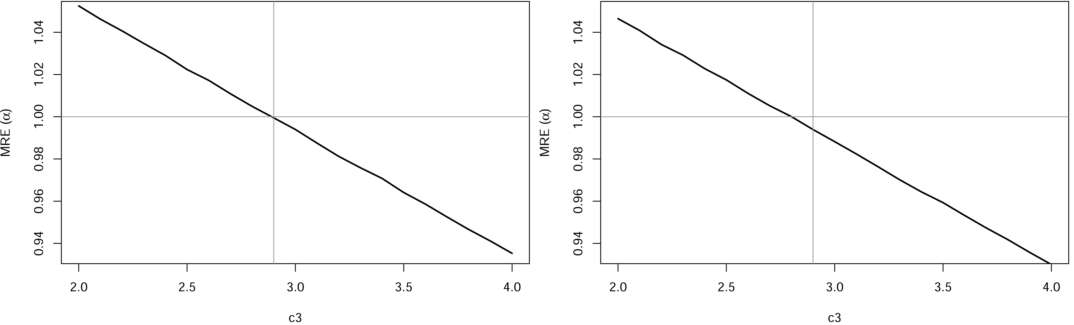
Recall that it was presented a class of MAP estimators for $\alpha$ that depends on $c_3$ . Therefore, before going on with the simulation study, it is necessary to find a value for $c_3$ in which the MRE is closer to one. Figure 2 presents the MREs for ${\alpha }_{MAP}$ considering different values of $c_3$ , for $\vartheta =(3,4)$ and $\vartheta =(10,4)$ and $n=20$ . We observed that a good choice is $c_3=2.9$ . Therefore, we considered such value in (28), where $n\ge 3$ . Since both estimators obtained from the reference posterior and the closed-form Bayes estimators came from the Bayesian approach, they will be referred to as Bayes and CBayes estimators, respectively. To achieve the MLEs, numerical techniques must be used to solve the non-linear equation (12), the uniroot function available in R was considered to find the estimate, and as provided theoretically, we find a unique solution in all situations.

Figure 2
MREs for $\alpha$ considering $c_3=(2,2.1,\cdots ,4)$ , $\alpha =3$ , $\lambda =4$ and $n=20$ (left panel) $\alpha =10$ , $\lambda =4$ and $n=20$ (right panel) for $N=100,000$ simulated samples.

Figure 3 shows the MREs, RMSEs and CPs for the estimates of $\alpha$ and $\lambda$ obtained by using the Monte Carlo (MC) method where $\alpha =(4,0.5)$ , $\lambda =2$ and $n=(15,20,\dots ,100)$ . The horizontal lines in the figures correspond to the minimum MREs and RMSEs, equal to one and zero, respectively. Notice that for $\lambda$ we have the same estimator using the three different estimators for complete data. In this case, both MRE and RMSE are similar. On the other hand, the confidence and credibility intervals are computed differently for each method. We observe that the estimates of the parameters are asymptotically unbiased, i.e., the MREs tend to one when $n$ increases and the RMSEs decrease to zero. However, the Bayes estimators, obtained from the reference posterior, outperform the other estimation procedures and present extremely efficient estimates for both parameters even for small sample sizes. It worth mentioning that if one needs fast computation, the CBayes returned similar estimates when compared to the Bayes estimators, obtained by considering reference priors.

Figure 3
MREs, RMSEs and CPs for $\alpha$ and \(\lambda\)$\lambda$ considering \(\alpha=4, \lambda=2\)$\alpha =4,\lambda =2$ (upper panel) and \(\alpha=0.5, \lambda=2\)$\alpha =0.5,\lambda =2$ (lower panel) for $N=100,000$ simulated samples and \(n=(15,20,\ldots,100)\)$n=(15,20,\dots ,100)$ .

5.2 - CENSORED DATA

In this section, we considered the Bayes estimators in the presence of randomly censored data. The censored data were generated as follows. We first generated two random samples of size $n$ , where $X\sim WH(\alpha ,\lambda )$ and $W\sim U(0,t_c)$ , with $t_c$ as fixed value. Then, from the obtained samples, we took $T_j=min(X_j,W_j),j=1,\dots ,n$ , and defined ${\delta }_j=0$ if $T_j=X_j$ or ${\delta }_j=1$ if $T_j=W_j$ .

Note that $t_c$ has to be selected in order to obtain the desired proportion of censoring. In order to obtain approximately $0.3$ and $0.5$ proportions of censored data, i.e., $30\%$ and $50\%$ of censorship we considered $t_c=9.3$ and $t_c=4.8$ , respectively. The simulation study is performed by considering $\vartheta =(2,4)$ , $N=100,000$ and $n=(20,25,\dots$ , $100)$ . To achieve the MLEs considering censored data the maxLik package to maximize the log-likelihood function (15). Different initial values were considered which returned the same estimates. Figure 4 shows the MREs, RMSEs and the coverage probabilities from the estimates of $\alpha$ and $\lambda$ obtained by using the MC method where $\alpha =4$ , $\lambda =2$ .

Figure 4
MREs, RMSEs and CPs for $\alpha$ and $\lambda$ considering $\alpha =4,\lambda =2$ for $N=100,000$ simulated samples, $30\%$ (upper panel) and $50\%$ (lower panel) of censoring and $n=(20,25,\dots ,100)$ .

The results indicate that the MLE of $\alpha$ has a systematic bias, as shown in Figure 4. On the other hand, from the Bayes estimators, we have observed more accurate results. The coverage probabilities are also close to the nominal levels as the MLE. Therefore, the Bayes estimators are also recommended to perform inference for the parameters of the WH distribution in the presence of censoring.

6 - PREDICTION ANALYSIS

In many application, we may be interested in identifying the time to the next event (failure). In these contexts, predicting future observations plays an important role, especially, when costs are linked with the events. In order to provide a predictive analysis of future events, we consider the Bayesian prediction with WH distribution using observed order statistics.

Several authors have performed prediction analysis from the Bayesian point of view (see, for instance, Pradhan and Kundu (2011), Kundu and Raqab (2012), Asgharzadeh et al. (2015)) for other distributions and the predictive distribution of future failure times and its respective credibility intervals.

We denote the order statistics of $T_1,\cdots ,T_m$ by $T_{(1)}<\dots <T_{(m)}$ . Let $T_{(m+1)}<\dots <T_{(n)}$ be the unobserved future sample and $t_{(m)}$ denote the $m$ -th order statistic. From the Markov property of the conditional order statistics, we have

$$\begin{array}{cc}\hfill f_{T_{m+k}}(y|𝐭)& =f_{T_{m+k}|T_m}(y|𝐭)\hfill \\ \hfill & =\frac{(n-m)!f(y){(F(y)-F(t_m))}^{k-1}(1-F(y){)}^{n-m-k}}{(k-1)!(n-m-k)!(1-F(t_m){)}^{n-m}},\hfill \end{array}$$ (32)

for $y>t_{(m)}$ . After some algebra we have

$$\begin{array}{cc}\hfill f_{T_{m+k}}(y|𝐭)=& \frac{3(n-m)!}{(k-1)!(n-m-k)!}{y}^{3\alpha -1}{\left(\frac{\alpha }{\lambda }\right)}^{\alpha }exp\left(\frac{\alpha }{\lambda }{y}^3\right)\hfill \\ \hfill & \times \frac{{(\gamma (\alpha ,\frac{\alpha }{\lambda }{y}^3)-\gamma (\alpha ,\frac{\alpha }{\lambda }{t}_m^3))}^{k-1}{\left(\Gamma (\alpha ,\frac{\alpha }{\lambda }{y}^3)\right)}^{n-m-k}}{{\left(\Gamma (\alpha ,\frac{\alpha }{\lambda }{t}_{(m)}^3)\right)}^{n-m}}.\hfill \end{array}$$ (33)

The posterior predictive density of $T_{(m+k)}$ given $𝐭$ is given by

$$p_{T_{m+k}}(y|𝐭)={\int }_0^{\infty }{\int }_0^{\infty }{f}_{T_{m+k}}(y|𝐭)p(\lambda ,\alpha |𝐭,𝛅)d\lambda d\alpha ,$$

where $p(\lambda ,\alpha |𝐭,𝛅)$ is given in (31). Consequently, the predictive density of $T_{(m+k)}$ according to $y>t_{(m)}$ is given by

$$f_{T_{m+k}}^{*}(y|𝐭)={\int }_0^{\infty }{\int }_0^{\infty }{f}_{T_{m+k}|T_m}(y|𝐭)p(\lambda ,\alpha |𝐭,𝛅)d\lambda d\alpha .$$ (34)

We also should note here that one striking result of the Bayesian predictive approach is the advantage in constructing a credibility interval for $T_{(m+k)}$ using the MCMC techniques.

7 - REAL-DATA APPLICATIONS

We examined the adjust of the proposed model on three real datasets to emphasize its flexibility and compare its performance with other distributions. A closer inspection of the following figures shows that the WH distribution exhibits best fit for each dataset when compared to commonly used distributions. In order to discriminate the best fit, we considered some key performance measures, namely, the Akaike information criterion (AIC) given by $AIC=-2l(\hat{\vartheta };x)+2p,$ the Corrected Akaike information criterion (AICc) given by $AICc=AIC+[2p(p+1)]/n-p-1,$ and the Bayesian information criterion (BIC) given by $BIC=plnn-2l(\hat{\vartheta };x),$ where $p$ is the dimension of $\vartheta$ and $\hat{\vartheta }$ is the estimate of the parameters and $l(\hat{\vartheta };x)$ is the logarithm of the likelihood function given in (8) and (14).

7.1 - LIFE TEST IN ELECTRICAL APPLIANCES

Table I presents a well-known dataset available in Lawless (2011), the number of 1000s of cycles to failure for a group of 60 electrical appliances in a life test, whose data are uncensored.

TABLE I
Failure times in 60 electrical appliances.

0.014	0.034	0.059	0.061	0.069	0.080	0.123	0.142
0.381	0.464	0.479	0.556	0.574	0.839	0.917	0.969
1.088	1.091	1.174	1.270	1.275	1.355	1.397	1.477
1.702	1.893	1.932	2.001	2.161	2.292	2.326	2.337
2.811	2.886	2.993	3.122	3.248	3.715	3.790	3.857
4.106	4.116	4.315	4.510	4.580	5.267	5.299	5.583
0.165	0.210	0.991	1.064	1.578	1.649	2.628	2.785
3.912	4.100	6.065	9.701

The results summarized in Table II show that the WH distribution is the best model since resulted in the lowest values of the different discrimination methods.

TABLE II
Results of AIC, AICc and BIC criteria for all fitted distributions considering the dataset related to the failure time of 60 electrical appliances.

Criteria	WH	Weibull	Gamma	Lognormal	Logistic
AIC	215.26	218.23	218.02	237.13	248.95
AICc	215.47	218.44	218.23	237.34	249.16
BIC	219.45	222.42	222.21	241.32	253.14

In order to discriminate the best fit, we considered the AIC, AICc, and BIC available in Table II. For the three criteria, we observed that the proposed model has smaller values, indicating a better fit for the WH distribution.

Table III provides the summary statistics: the MAP estimates, standard-deviations (SD) and 95% credibility intervals (CI) for $\alpha$ , $\lambda$ and $y^{*}$ (future failure time). We can obtain the MAP estimates of the parameters $\lambda$ and $\alpha$ from (26) and (28), respectively. In order to predict the future failures of an item, as described in Section 6, we considered the posterior predictive density of $T_{m+k}$ from (34).

TABLE III
MAPs, SDs and 95% CIs for α, λ and y^* related to the WH distribution.

ϑ	MAP	SD	CI95%ϑ
α	0.2132	0.0306	(0.1593; 0.2772)
λ	43.7261	15.7220	(28.3993; 87.6349)
y*	9.9075	0.6349	(9.7185; 12.1094)

As can be seen from Table I, the last failure was observed at 9.701 cycles. Then, the last line of Table III shows the prediction of the 61st failure will be at $y^{*}=9.908$ cycles with 95% predictive interval given by (9.7185; 12.1094).

7.2 - FAILURE TIME DATA OF ELECTRICAL COMPONENTS

The following datasets motive the application of WH distribution in the presence of censored data. The first dataset concerns electrical failures in the components from agricultural machines. The follow-up time was a harvesting season. In this period, the electrical components have failed 29 times collected in 2017. The data are shown in Table IV.

TABLE IV
Dataset related to the agricultural machines with failure in electrical components (+ indicates censoring).

1	1	1	2	2	2	2	4	6	8	8
9	11	12	15	21	21	21	21	23	24	27
29	31	36	39	41	45	46	47+	47+

In order to discriminate the best fit, we used the AIC, AICc, and BIC (see Table V). In all of them, the proposed model has smaller values, indicating a better fit.

TABLE V
Results of AIC, AICc and BIC criteria for all fitted distributions considering the dataset related to the agricultural machine’s components electrical problems.

Criteria	WH	Weibull	Gamma	Lognormal	Logistic
AIC	236.57	238.01	237.80	241.34	255.41
AICc	237.03	238.47	238.26	241.80	255.87
BIC	239.31	240.74	240.53	244.00	258.14

Table VIprovides the summary statistics: the MAP estimates, SDs and 95% CIs for $\alpha$ , $\lambda$ and $y^{*}$ (future failure time). As can be seen from the Table IV the last failure was observed on the ${46}^{t}h$ day. Then from the last line of Table VI we can see the prediction of the ${47}^{t}h$ failure that will be at \(50.13\)$50.13$ days, with a 95% predictive interval given by (47.27; 78.25).

TABLE VI
MAPs, SDs and 95% CIs for α, λ and y^* related to the WH distribution.

ϑ	MAP	SD	CI95%ϑ
α	0.2239	0.0480	( 0.1521; 0.3435)
λ	27733.5	7654.4	(12949.92; 42160.68)
y*	50.1313	8.3780	(47.2707; 78.2493)

Turning now to another type of failure, Table VII presents the time up to corrective maintenance of the agricultural machine. In this case, correctly predicting the next maintenance is of main interest in order to reduce costs.

TABLE VII
Dataset related to the agricultural machine’s corrective maintenance (+ indicates censoring).

1	1	1	1	1	1	1	2	2	3	3	3
3	3	4	4	4	4	4	4	4	5	5	5
5	5	5	5	5	5	6	6	6	6	6	6
6	6	6	6	6	6	6	6	6	6	6	6
7	7	7	7	7	7	7	7	7	7	7	7
7	7	8	8	8	8	8	8	8	8	8	8
8	9	9	9	9	9	11	11	11	11	11	11
11	11	13	13+	13+

From the results presented in Table VIII we observe from the AIC, AICc and BIC that the WH distribution returned better fit for the dataset.

TABLE VIII
Results of AIC, AICc and BIC criteria for all fitted distributions considering the dataset related to the agricultural machine’s revision.

Criteria	WH	Weibull	Gamma	Lognormal	Logistic
AIC	441.29	442.52	451.37	469.56	442.29
AICc	441.43	442.66	451.51	469.70	442.43
BIC	446.26	447.50	456.34	474.53	447.27

Table Table IXshows the MAPs, standard deviations, and 95% credible intervals for the parameters of the WH distribution. From Table VII the last failure was observed at 13 days. Applying the proposed methodology, the prediction of the 31st maintenance will be at 13.37 days with 95% predictive interval given by (13.03;16.83).

TABLE IX
MAPs, SDs and 95% CIs for α, λ and y^* related to agricultural machine’s revision dataset.

ϑ	MAP	SD	CI95%ϑ
α	0.6309	0.0793	(0.4892; 0.7949)
λ	423.5057	60.1510	(332.7807; 564.9964)
y*	13.3713	1.0384	(13.0293; 16.8254)

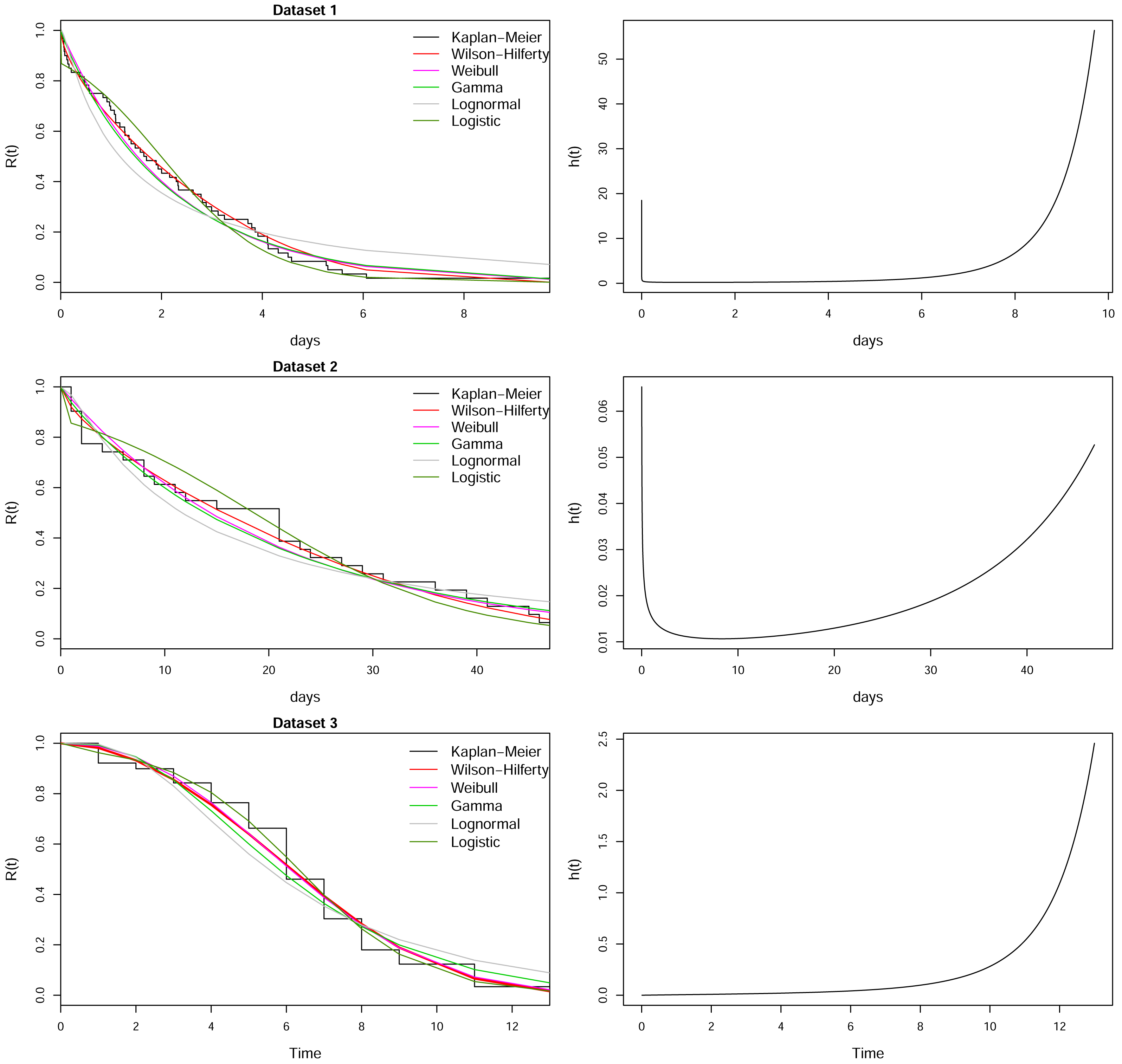
Figure 5presents the reliability function fitted by different distributions and the Kaplan-Meier curve for the three data sets. In all cases, the WH distribution provides an improved fit for the datasets.

Figure 5
Reliability function adjusted by different distributions superimposed to the empirical reliability function. Right-hand panel: Estimated hazard function.

Therefore, the practical importance of the WH distribution is observed for these datasets, since it provides a better fitting in comparison with other essential distributions, allowing to conduct prevision for the next failures.

8 - CONCLUSIONS

In this paper, we revisit the WH distribution and presented mathematical properties of this important distribution, which can be used in situations where the data present bathtub or increasing hazard rate. Initially, the parameter estimators and their asymptotic intervals were explored using the maximum likelihood theory under complete and censored data. Further, we considered an objective Bayesian analysis with an overall reference prior in order to obtain improved estimators, which outperform the ones obtained via maximum likelihood. It is proved that the reference posterior distribution is proper when $n\ge 1$ and the resulting marginal posterior intervals have accurate frequentist coverage. Moreover, we have introduced MAP estimators for the parameters of WH distribution that have closed-form expressions. A simulation study revealed the superiority of the Bayes estimators.

A Bayes prediction of the future failure time was also presented based on observed order statistics. The proposed methodology was applied to three data sets associated with failure time. Many possible extensions of this current work can be considered. This distribution is a promising distribution to be used in studies involving recurrent event data. In this case, we can consider a rate model from a nonhomogeneous Poisson process, where the parametric baseline rate function is a WH rate function. Further, classical point prediction could be studied for this model, for example, maximum likelihood prediction, best-unbiased predictor, conditional median prediction along with prediction interval using Pivotal method and highest conditional density (HCD) method. Our approach should be investigated further in this context.

ACKNOWLEGMENTS

The authors are very grateful to the Editor and the three reviewers for their helpful and useful comments that improved the manuscript. This study was financed in part by the Coordenação de Aperfeiçoamento de Pessoal de Nível Superior (CAPES) and Conselho Nacional de Desenvolvimento Científico e Tecnológico (CNPq). Pedro L. Ramos is grateful to the Fundação de Amparo à Pesquisa do Estado de São Paulo (FAPESP, Proc. 2017-25971-0).

REFERENCES

• ASGHARZADEH A, VALIOLLAHI R and KUNDU D. 2015. Prediction for future failures in weibull distribution under hybrid censoring. J Stat Comput Simul 85(4): 824-838.
• BERGER JO et al. 2015. Overall objective priors. Bayesian Anal 10(1): 189-221.
• BERNARDO JM. 1979. Reference posterior distributions for bayesian inference. J Royal Stat Soc Series B, p. 113-147.
• BERNARDO JM. 2005. Reference analysis. Handbook of Statistics 25: 17-90.
• COX DR and REID N. 1987. Parameter orthogonality and approximate conditional inference. J Royal Stat Society Series B 49(1): 1-18.
• CRAIN BR and MORGAN RL. 1975. Asymptotic normality of the posterior distribution for exponential models. Ann Stat, p. 223-227.
• DEY S, MAZUCHELI J and NADARAJAH S. 2018. Kumaraswamy distribution: different methods of estimation. J Comput Appl Math 37(2): 2094-2111.
• FOLLAND GB. 1999. Real analysis: modern techniques and their applications. Wiley, New York, 2^nd edition.
• ISHIKAWA T, TOTANI T, NISHIMICHI T, TAKAHASHI R, YOSHIDA N and TONEGAWA M. 2014. On the systematic errors of cosmological-scale gravity tests using redshift-space distortion: non-linear effects and the halo bias. Mon Notices Royal Astron Soc 443(4): 3359-3367.
• KHODABIN M and AHMADABADI A. 2010. Some properties of generalized gamma distribution. Math Sci 4(1): 9-28.
• KUNDU D and RAQAB MZ. 2012. Bayesian inference and prediction of order statistics for a type-ii censored Weibull distribution. J Stat Plan Inference 142(1): 41-47.
• LAWLESS JF. 2011. Statistical models and methods for lifetime data. Volume 362, J Wiley \& Sons.
• LOUZADA F, RAMOS PL and NASCIMENTO D. 2018. The inverse nakagami-m distribution: A novel approach in reliability. IEEE Trans Rel (99): 1-13.
• LOUZADA F, RAMOS PL and RAMOS E. 2019. A note on bias of closed-form estimators for the gamma distribution derived from likelihood equations. Am Stat, p. 1-8.
• PRADHAN B and KUNDU D. 2011. Bayes estimation and prediction of the two-parameter gamma distribution. J Stat Comp Simul 81(9): 1187-1198.
• RAMOS PL, ACHCAR JA, MOALA FA, RAMOS E and LOUZADA F. 2017. Bayesian analysis of the generalized gamma distribution using non-informative priors. Statistics 51(4): 824-843.
• RAMOS PL, LOUZADA F and RAMOS E. 2018. Posterior properties of the nakagami-m distribution using noninformative priors and applications in reliability. IEEE Trans Rel 67(1): 105-117.
• STACY EW. 1962. A generalization of the gamma distribution. Ann Math Stat, p. 1187-1192.
• TEIMOURI M, HOSEINI SM and NADARAJAH S. 2013. Comparison of estimation methods for the weibull distribution. Statistics 47(1): 93-109.
• TIBSHIRANI R. 1989. Noninformative priors for one parameter of many. Biometrika 76(3): 604-608.
• WILSON EB and HILFERTY MM. 1931. The distribution of chi-square. Proc Natl Acad Sci 17(12): 684-688.
• ZEMZAMI M and BENAABIDATE L. 2016. Improvement of artificial neural networks to predict daily streamflow in a semi-arid area. Hydrol Sci J 61(10): 1801-1812.

Publication Dates

• Publication in this collection
  19 Aug 2019
• Date of issue
  2019

History

• Received
  02 Jan 2019
• Accepted
  10 June 2019