Singular surfaces of revolution with prescribed unbounded mean curvature

Abstract

Abstract: We give an explicit formula for singular surfaces of revolution with prescribed unbounded mean curvature. Using this mean curvature, we give conditions for certain types of singularities of those surfaces. Periodicity of that surface is also discussed.

Key words
Cuspidal edge; mean curvature; periodicity surface of revolution; cusps

INTRODUCTION

In this note, we study surfaces of revolution with singular points. Let $I\subset 𝐑$ be an open interval, and $\gamma :I\to {𝐑}^2$ a $C^{\infty }$ -map. We set $\gamma (t)=(x(t),y(t))$ $(y>0)$, and parametrize the surface of revolution $M$ of $\gamma$ by

$$s(t,\vartheta )=(x(t),y(t)cos\vartheta ,y(t)sin\vartheta ).$$ 0.1

The curve $\gamma$ is called the profile curve or the generating curve of $s$. We denote by $H(t)$ the mean curvature of $s(t,\vartheta )$. Given a $C^{\infty }$ function $H(t)$ on $I$, it is given by Kenmotsu (Kenmotsu 1980) that an explicit generating curve $(x(t),y(t))$ satisfying the surface of revolution $s(t,\vartheta )$ has the mean curvature $H(t)$ on the set of its regular points, and $t$ is an arc-length parameter of $(x(t),y(t))$. Moreover, the periodicity of $s$ is also studied by Kenmotsu (Kenmotsu 2003).

On the other hand, in recent decades, there are several articles concerning the differential geometry of singular curves and surfaces, namely, curves and surfaces with singular points. Among them, we cite Bruce and West 1998, Fukui and Hasegawa 2012, Fukunaga and Takahashi 2014, Honda et al. 2019, Izumiya et al. 2016, Martins et al. 2016, Naokawa et al. 2016, Oset Sinha and Tari 2018, Saji et al. 2009, Shiba and Umehara 2012, (A. Honda et al., unpublished data). If the generating curve $\gamma$ is regular, then the mean curvature $H$ is differentiable on $I$, but if $\gamma$ has a singularity, then $H$ may diverge (Saji et al. 2009, Martins et al. 2016). Given a $C^{\infty }$ function $H$ defined on $I\backslash P$, where $P$ is a discrete set, we give an explicit generating curve $\gamma =(x,y)$ such that the mean curvature of the surface of revolution of $\gamma$ coincides with the function $H$ on the set of regular points. We also give conditions for the generic singularities of $\gamma$ and discuss the periodicity of the surface.

1 - CONSTRUCTION OF SINGULAR SURFACES OF REVOLUTION

Let $I\subset 𝐑$ be an open interval, and let $\gamma :I\to {𝐑}^2$ be a $C^{\infty }$ map. We set $\gamma (t)=(x(t),y(t))$, and assume $y(t)>0$ for any $t\in I$. We assume that there exists a $C^{\infty }$ map $\phi :I\to 𝐑$ such that $\gamma \prime (t)$ and $(cos\phi (t),sin\phi (t))$ are linearly dependent for all $t\in I$. Then we have a function $\mathit{\text{𝑙}}:I\to 𝐑$ such that

$$\gamma \prime (t)=\mathit{\text{𝑙}}(t)e(t),e(t)=(cos\phi (t),sin\phi (t)).$$

This condition is equivalent to $\gamma$ being a frontal (see Section 2 for detail). We choose the following unit normal vector of the surface of revolution $M$ of $\gamma$

$$\nu (t,\vartheta )=(sin\phi (t),-cos\phi (t)cos\vartheta ,-cos\phi (t)sin\vartheta ).$$ (1.1)

One can compute the mean curvature $H$ on $M\backslash \{s(t,\vartheta )|\mathit{\text{𝑙}}(t)=0\}$, namely the set of regular points of $M$, using $\nu$ in (1.1). We find that:

$$H(t)={\displaystyle \frac{1}{2}}({\displaystyle \frac{cos\phi (t)}{y(t)}}-{\displaystyle \frac{\phi \prime (t)}{\mathit{\text{𝑙}}(t)}}),$$

where $\prime =d/dt$.

Lemma 1.1. The function $H\mathit{\text{𝑙}}$ can be extended to a $C^{\infty }$ function on $I$.

Proof. It follows from the above expression of $H$ and the assumption $y>0$.

By the above expression, $\phi \prime$ relates the boundedness of the mean curvature. See Martins et al. 2016, Proposition 3.8 for detailed boundedness of the mean curvature for the case of cuspidal edges. Since $|\gamma \prime |=|\mathit{\text{𝑙}}|$, the function $\mathit{\text{𝑙}}$ is the same as the half-arclength parameter (Shiba and Umehara 2012) near a point $t_0$ satisfying $\gamma \prime (t_0)=0$, $\gamma ″(t_0)\ne 0$ up to a constant. We remark that the case $y=0$ is already considered in Kenmotsu 1980.

Conversely, suppose given a $C^{\infty }$ function $H:I\backslash P\to 𝐑$, where $P$ is a discrete set, and a function $\mathit{\text{𝑙}}:I\to 𝐑$ such that $H\mathit{\text{𝑙}}$ is a $C^{\infty }$ function on $I$ and ${\mathit{\text{𝑙}}}^{-1}(0)=P$. We ask if there is a surface of revolution $M$ with a generating curve $\gamma (t)=(x(t),y(t))$ such that

$$(x\prime (t),y\prime (t))=\mathit{\text{𝑙}}(t)(cos\phi (t),sin\phi (t))$$ (1.2)

and mean curvature $H$ with respect to(1.1). By Lemma Lemma 1.1, $x,y$ satisfy the differential equation

$$2H(t)\mathit{\text{𝑙}}(t)y(t)-\mathit{\text{𝑙}}(t)cos\phi (t)+y(t)\phi \prime (t)=0.$$ (1.3)

Following Kenmotsu 1980, we have the following theorem.

Theorem 1.2. A general solution of the differential equation (1.3) with the condition(1.2) is

$y(t)=((F(t)-c_1{)}^2+(G(t)-c_2{)}^2{)}^{1/2},$ (1.4)

$$\begin{array}{cc}\hfill x\prime (t)& ={\displaystyle \frac{F\prime (t)(G(t)-c_2)-G\prime (t)(F(t)-c_1)}{((F(t)-c_1{)}^2+(G(t)-c_2{)}^2{)}^{1/2}}}\hfill \\ \hfill & ={\displaystyle \frac{F\prime (t)(G(t)-c_2)-G\prime (t)(F(t)-c_1)}{y(t)}},\hfill \end{array}$$ (1.5)

where

$$F(t)={\int }_0^t\mathit{\text{𝑙}}(u)sin\eta (u)du,G(t)={\int }_0^t\mathit{\text{𝑙}}(u)cos\eta (u)du,\eta (u)={\int }_0^{u}2H(v)\mathit{\text{𝑙}}(v)dv.$$ (1.6)

We take the initial values $c_1,c_2$ satisfying that $(F(t)-c_1{)}^2+(G(t)-c_2{)}^2>0$ on $t\in I$.

Proof. We set $z(t)=y(t)sin\phi (t)+iy(t)cos\phi (t)$, with $i^2=-1$ (cf. Kenmotsu 1980, p. 148). Then by (1.2),

$$\begin{array}{cc}\hfill z\prime & =y\prime sin\phi +y\phi \prime cos\phi +i(y\prime cos\phi -y\phi \prime sin\phi )\hfill \\ \hfill & =\mathit{\text{𝑙}}{sin}^2\phi +y\phi \prime cos\phi +i(\mathit{\text{𝑙}}sin\phi cos\phi -y\phi \prime sin\phi ).\hfill \end{array}$$

On the other hand, by (1.3),

$$2iH\mathit{\text{𝑙}}z=-(\mathit{\text{𝑙}}cos\phi -y\phi \prime )cos\phi +i(\mathit{\text{𝑙}}cos\phi -y\phi \prime )sin\phi .$$

Thus (1.3) can be written as

$$z\prime (t)-2iH(t)\mathit{\text{𝑙}}(t)z(t)-\mathit{\text{𝑙}}(t)=0,$$

and a general solution of this equation is

$\begin{array}{c}z(t)=(F(t)-c_1)\sin \eta (t)+(G(t)-c_2)\cos \eta (t)\\ +i((G(t)-c_2)\sin \eta (t)-(F(t)-c_1)\cos \eta (t)),\end{array}$

where $c_1,c_2\in 𝐑$, and $F,G,\eta$ are the functions as in (1.6). Using the fact that $y(t{)}^2=|z(t){|}^2$ and $x\prime (t)=\mathit{\text{𝑙}}(t)cos\phi (t)=\mathit{\text{𝑙}}(t)(z(t)-\bar{z}(t))/(2iy(t))$, we get the assertion.

We remark that in the formula (1.4), by

$$y\prime =\mathit{\text{𝑙}}sin(\eta +\alpha ),\alpha =arcsin{\displaystyle \frac{G(t)-c_2}{\sqrt{(F(t)-c_1{)}^2+(G(t)-c_2{)}^2}}},$$

we see that $\phi =\eta +\alpha +2\pi n$, where $n$ is an integer. It should be mentioned that on the set of regular points on $M$, there is a result of Kenmotsu 1980, (see also Kenmotsu 1979), and cusp points can be considered by taking the limits of regular parts. However, in Section 2, we exhibit a class of singularities of $\gamma$, which cannot be investigated by considering limits of regular points. Furthermore, the formulae (1.4), (1.5) include singular points in the interior points of the domain. Thus they can extend the treatment of singular surfaces of revolution. We remark that there is a formula which represents immersed surfaces (see Kenmotsu 1979, Theorem 4) by means of prescribed mean curvature and unit normal vector.

2 - SINGULARITIES OF GENERATING CURVES

In this section, we consider the relation between singularities of generating curves and of the surfaces of revolution. Let $U$ be an open domain of ${𝐑}^m$, and let $f:U\to {𝐑}^n$ be a $C^{\infty }$ map $(m\le n)$. A point $p\in U$ is a singular point of $f$ if $rankd{f}_p<m$. A singular point $p$ of $\gamma :I\to {𝐑}^2$ is called an ordinary cusp or a$3/2$-cuspif the map-germ $\gamma$ at $p$ is $𝒜$ -equivalent to $t\mapsto (t^2,t^3)$ at $0$. (Two map-germs $f_1,f_2:({𝐑}^m,0)\to ({𝐑}^n,0)$ are $𝒜$ -equivalent if there exist diffeomorphisms $S:({𝐑}^m,0)\to ({𝐑}^m,0)$ and $T:({𝐑}^n,0)\to ({𝐑}^n,0)$ such that $f_2\circ S=T\circ f_1$.) Similarly, a singular point $p$ of $\gamma$ is called a $j/i$ -cusp, $(i,j)=(2,5),(3,4),(3,5)$, if the map-germ $\gamma$ at $p$ is $𝒜$-equivalent to $t\mapsto (t^i,t^j)$ at $0$. It is known that the singularities of a map-germ $(𝐑,0)\to ({𝐑}^2,0)$ which are determined by their $5$ -jets with respect to $𝒜$-equivalence are only the above cusps. Recognition criteria for these singularities are known, see for example Bruce and Gaffney (1982).

Fact 2.1.$($ Recognition criteria $)$ A singularity of $\gamma :(𝐑,p)\to ({𝐑}^2,0)$ is

• a $3/2$-cusp if and only if $det(\gamma ″,\gamma ‴)\ne 0$ at $p$.

• a $5/2$-cusp if and only if $\gamma ″\ne 0$, $\gamma ‴=k\gamma ″$, $($ namely, $det(\gamma ″,\gamma ‴)=0)$ and $det(\gamma ″,3{\gamma }^{(5)}-10k{\gamma }^{(4)})\ne 0$ at $p$.

• a $4/3$ -cusp if and only if $\gamma ″=0$ and $det(\gamma ‴,{\gamma }^{(4)})\ne 0$ at $p$.

• a $5/3$ -cusp if and only if $\gamma ″=0$, $det(\gamma ‴,{\gamma }^{(4)})=0$ and $det(\gamma ‴,{\gamma }^{(5)})\ne 0$ at $p$.

A map-germ $\gamma$ at $p$ is called frontal if there exists a map $n:(𝐑,p)\to ({𝐑}^2,0)$ satisfying $|n|=1$ and $\gamma \prime \cdot n=0$ for all $t$ near $p$. A frontal is a front at $p$ if the pair $(\gamma ,n)$ is an immersion into ${𝐑}^2\times S^1$ at $p$, where $S^1$ is the unit circle in ${𝐑}^2$. If $\gamma$ at $p$ is a $3/2$-cusp or a $4/3$ -cusp then it is a front, and if $\gamma$ at $p$ is a $5/2$ -cusp or a $5/3$ -cusp then it is a frontal but not a front. By definition, $\gamma \prime (p)=0$ if and only if $\mathit{\text{𝑙}}(p)=0$. We have the following:

Proposition 2.2. The curve $\gamma =(x,y)$ given by (1.4), (1.5) is a frontal at any point $t\in I$. Moreover, if $\mathit{\text{𝑙}}(p)=0$, then $\gamma$ at $p$ is a front if and only if $\eta \prime (p)\ne 0$.

Proof. Since $y\prime =(F\prime (F-c_1)+G\prime (G-c_2))y^{-1},$ we have

${\gamma }^{\prime }={\displaystyle \frac{F^{\prime }}{y}}\left(\begin{array}{c}G-c_2\\ F-c_1\end{array}\right)U,+{\displaystyle \frac{G^{\prime }}{y}}\left(\begin{array}{c}-(F-c_1)\\ G-c_2\end{array}\right)={\displaystyle \frac{\mathit{\text{l}}\cos \eta }{y}}U+{\displaystyle \frac{\mathit{\text{l}}\sin \eta }{y}}\left(\begin{array}{cc}0& 1\\ -1& 0\end{array}\right)U={\displaystyle \frac{\mathit{\text{l}}}{y}}{R}_{-\eta }U,$ (2.1)

where

$$\gamma \prime =\left(\begin{array}{c}\hfill x\prime \hfill \\ \hfill y\prime \hfill \end{array}\right),U=\left(\begin{array}{c}\hfill -(F-c_1)\hfill \\ \hfill G-c_2\hfill \end{array}\right)\mathrm{\text{and}}{R}_{-\eta }=\left(\begin{array}{cc}\hfill cos(-\eta )\hfill & \hfill -sin(-\eta )\hfill \\ \hfill sin(-\eta )\hfill & \hfill cos(-\eta )\hfill \end{array}\right).$$

We set $n=R_{-\eta +\pi /2}U/|U|$. Then $|n|=1$ and $n$ is perpendicular to $\gamma \prime$. Thus $\gamma$ is a frontal. Let us assume $\mathit{\text{𝑙}}(p)=0$. Then $\gamma$ at $p$ is a front if and only if $n\prime (p)\ne 0$. This is equivalent to saying that $R_{-\eta +\pi /2}U$ and $(R_{-\eta +\pi /2}U)\prime$ are linearly independent. Since $\mathit{\text{𝑙}}(p)=0$, it holds that $(R_{-\eta +\pi /2}U)\prime (p)=(R_{-\eta +\pi /2})\prime (p)U(p)$, and $(R_{-\eta +\pi /2})\prime =-\eta \prime R_{-\eta +\pi }$, we see that $n\prime (p)\ne 0$ is equivalent to $\eta \prime (p)\ne 0$. This proves the assertion.

Moreover, we have the following:

Proposition 2.3. Let $\gamma =(x,y)$ be given by (1.4) and (1.5), and suppose $\mathit{\text{𝑙}}(p)=0$. Then $\gamma$ at $p$ is

1. a $3/2$ -cusp if and only if $\mathit{\text{𝑙}}\prime \eta \prime \ne 0$ holds at $p$,

2. a $5/2$ -cusp if and only if $\mathit{\text{𝑙}}\prime \ne 0$, $\eta \prime =0$ and $\mathit{\text{𝑙}}″\eta ″-\mathit{\text{𝑙}}\prime \eta ‴\ne 0$ hold at $p$,

3. a $4/3$ -cusp if and only if $\mathit{\text{𝑙}}\prime =0$ and $\eta \prime \mathit{\text{𝑙}}″\ne 0$ hold at $p$,

4. a $5/3$ -cusp if and only if $\mathit{\text{𝑙}}\prime =\eta \prime =0$ and $\eta ″\mathit{\text{𝑙}}″\ne 0$ hold at $p$.

Proof. By (2.1), we have

$$\gamma ″=\mathit{\text{𝑙}}\prime \left(y^{-1}\right)R_{-\eta }U+\mathit{\text{𝑙}}\left(y^{-1}\right)\prime R_{-\eta }U+\mathit{\text{𝑙}}\left(y^{-1}\right)(R_{-\eta })\prime U+\mathit{\text{𝑙}}\left(y^{-1}\right)R_{-\eta }U\prime$$ (2.2)

and since $\mathit{\text{𝑙}}(p)=0$, so $y\prime (p)=0$ and $U\prime (p)=0$ hold. Then we have $\gamma ″(p)=\mathit{\text{𝑙}}\prime (p)y(p{)}^{-1}{R}_{-\eta }(p)U(p)$. Thus $\gamma ″(p)\ne 0$ if and only if $\mathit{\text{𝑙}}\prime (p)\ne 0$. We assume that $\mathit{\text{𝑙}}\prime (p)\ne 0$. Then by (2.2),

$$\gamma ‴=\mathit{\text{𝑙}}″\left(y^{-1}\right)R_{-\eta }U+\mathit{\text{𝑙}}\left(y^{-1}\right)″R_{-\eta }U+\mathit{\text{𝑙}}\left(y^{-1}\right)(R_{-\eta })″U+\mathit{\text{𝑙}}\left(y^{-1}\right)R_{-\eta }U″$$ (2.3)

$$\begin{array}{cc}\hfill & +2\mathit{\text{𝑙}}\prime \left(y^{-1}\right)\prime R_{-\eta }U+2\mathit{\text{𝑙}}\prime \left(y^{-1}\right)(R_{-\eta })\prime U+2\mathit{\text{𝑙}}\prime \left(y^{-1}\right)R_{-\eta }U\prime \hfill \\ \hfill & +2\mathit{\text{𝑙}}\left(y^{-1}\right)\prime (R_{-\eta })\prime U+2\mathit{\text{𝑙}}\left(y^{-1}\right)\prime R_{-\eta }U\prime +2\mathit{\text{𝑙}}\left(y^{-1}\right)(R_{-\eta })\prime U\prime ,\hfill \end{array}$$

and since $\mathit{\text{𝑙}}(p)=y\prime (p)=0$, $U\prime (p)=0$, and $(R_{-\eta })\prime =-\eta \prime R_{-\eta +\pi /2}$,

$$\gamma ‴=(\mathit{\text{𝑙}}″R_{-\eta }U+2\mathit{\text{𝑙}}\prime (R_{-\eta })\prime U)y^{-1}=(\mathit{\text{𝑙}}″R_{-\eta }U+2\mathit{\text{𝑙}}\prime (-\eta \prime )R_{-\eta +\pi /2}U)y^{-1}$$

holds at $p$. Hence $det(\gamma ″,\gamma ‴)(p)\ne 0$ if and only if $\eta \prime (p)\ne 0$, and this proves (1). We assume $\eta \prime (p)=0$. Then we see $k$ in Fact 2.1,(2) (namely, $\gamma ‴(p)=k\gamma ″(p)$ ) is $k=\mathit{\text{𝑙}}″(p)/\mathit{\text{𝑙}}\prime (p)$.

Now we calculate $det(\gamma ″,3{\gamma }^{(5)}-10k{\gamma }^{(4)})(p)$. Differentiating(2.2), with $\mathit{\text{𝑙}}(p)=y\prime (p)=\eta \prime (p)=0$ and $U\prime (p)=0$, we get

$\begin{array}{c}{\gamma }^{(4)}=3{\mathit{\text{l}}}^{\prime }(y^{-1}{R}_{-\eta }{U}^{″}+y^{-1}(R_{-\eta }{)}^{″}U+(y^{-1}{)}^{″}{R}_{-\eta }U)+y^{-1}{\mathit{\text{l}}}^{‴}{R}_{-\eta }U,\\ k{\gamma }^{(4)}=3{\mathit{\text{l}}}^{″}(y^{-1}{R}_{-\eta }{U}^{″}+y^{-1}(R_{-\eta }{)}^{″}U+(y^{-1}{)}^{″}{R}_{-\eta }U)+y^{-1}{\mathit{\text{l}}}^{‴}{\mathit{\text{l}}}^{″}{R}_{-\eta }U/{\mathit{\text{l}}}^{\prime },\\ {\gamma }^{(5)}=4{\mathit{\text{l}}}^{\prime }(y^{-1}{R}_{-\eta }{U}^{‴}+y^{-1}(R_{-\eta }{)}^{‴}U+(y^{-1}{)}^{‴}{R}_{-\eta }U)\\ +6{\mathit{\text{l}}}^{″}(y^{-1}{R}_{-\eta }{U}^{″}+y^{-1}(R_{-\eta }{)}^{″}U+(y^{-1}{)}^{″}{R}_{-\eta }U)+y^{-1}{\mathit{\text{l}}}^{(4)}{R}_{-\eta }U\end{array}$

at $p$. Thus

$$3{\gamma }^{(5)}-10k{\gamma }^{(4)}=12(\mathit{\text{𝑙}}\prime ((R_{-\eta })‴U+R_{-\eta }U‴)-\mathit{\text{𝑙}}″((R_{-\eta })″U+R_{-\eta }U″))y^{-1}+\beta R_{-\eta }U$$

holds at $p$, where $\beta$ is a real number. It follows that $det(\gamma ″,3{\gamma }^{(5)}-10k{\gamma }^{(4)})(p)=12\mathit{\text{𝑙}}\prime (p)(\mathit{\text{𝑙}}″(p)\eta ″(p)-\mathit{\text{𝑙}}\prime (p)\eta ‴(p))$. This proves the assertion(2).

Next we assume $\gamma ″(p)=0$, namely, $\mathit{\text{𝑙}}\prime (p)=0$. Then by (2.3),

$$\gamma ‴=\mathit{\text{𝑙}}″(y^{-1})R_{-\eta }U,{\gamma }^{(4)}=3\mathit{\text{𝑙}}″(y^{-1})(R_{-\eta })\prime U+\mu R_{-\eta }U$$

for some scalar $\mu$. Since $(R_{-\eta })\prime =-\eta \prime R_{-\eta +\pi /2}$, this proves (3).

We assume that $\eta \prime (p)=0$. Differentiating (2.3),

$${\gamma }^{(5)}=6\mathit{\text{𝑙}}″((R_{-\eta })″U+R_{-\eta }U″)y^{-1}+\tau R_{-\eta }U$$

at $p$, where $\tau$ is a real number. Since $U^{″}={\mathit{\text{l}}}^{\prime }{\phantom{(-\sin \eta ,\cos \eta )}}^t(-\sin \eta ,\cos \eta )+\mathit{\text{l}}{\phantom{(-\sin \eta ,\cos \eta {)}^{\prime }}}^t(-\sin \eta ,\cos \eta {)}^{\prime }=0$ at $p$, we have (4), where ${\phantom{v}}^{t}v$ stands for the transpose of the vector $v$.

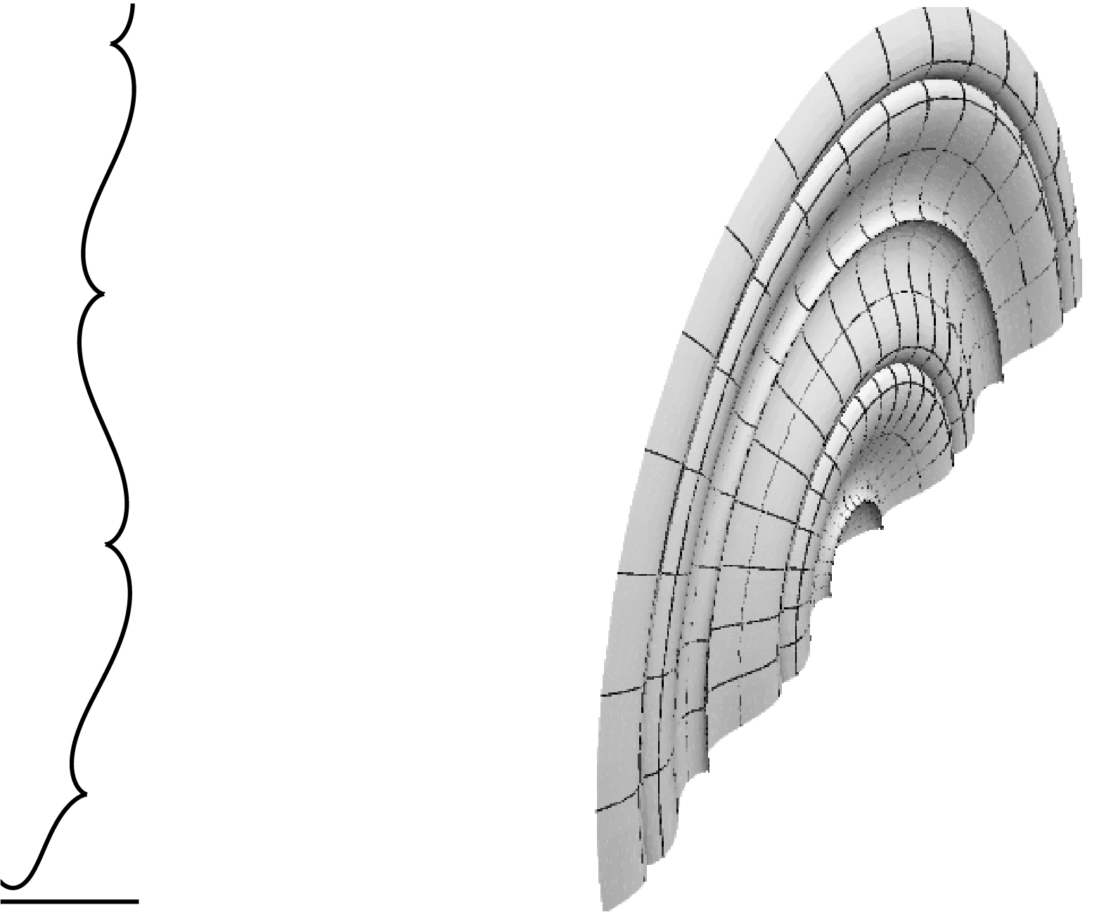
Example 2.4. We set $H=1/t$ and $\mathit{\text{𝑙}}=t$ with $c_1=c_2=1/10$. By Proposition 2.3, $\gamma$ at $t=0$ is a $3/2$-cusp. The generating curve is as in Figure 1.

Figure 1
The generating curve left and the surface of revolution of Example 2.4. The horizontal line is the axis of rotation.

Example 2.5. We consider the following examples.

1. $H=1+t$, $\mathit{\text{𝑙}}=t$, $c_1=c_2=1/10$. Then $\gamma$ is a $5/2$-cusp (Figure 2, (a1)).

2. $H=1/t^2$, $\mathit{\text{𝑙}}=t^2$, $c_1=c_2=1/10$. Then $\gamma$ is a $4/3$-cusp (Figure 2, (a2)).

3. $H=1/t$, $\mathit{\text{𝑙}}=t^2$, $c_1=c_2=1/10$. Then $\gamma$ is a $5/3$-cusp (Figure 2, (a3)).

Figure 2
Above: The generating curves of Example 2.5. The horizontal lines are the axes of rotation. Below: The surfaces of revolution of Example 2.5

In Figure 2, the singular points of these curves are indicated by the arrows. The surfaces of revolution of these examples are in Figure 2, botom, (b1), (b2) and (b3) respectively.

We consider now the singularities of the surface of revolution with $\gamma$ as in Proposition 2.3. A singular point $q$ of a map $f:({𝐑}^2,q)\to ({𝐑}^3,0)$ is called a $j/i$-cuspidal edge if $f$ at $q$ is $𝒜$ -equivalent to $f_{ij}:(u,v)\mapsto (u^i,u^j,v)$ at $0$. It holds that the map-germ $s$ in (0.1) at (p, $\vartheta$) is a $j/i$ -cuspidal edge if and only if the generating curve $\gamma =(x(u),y(u))$ at $p$ is a $j/i$-cusp. We see this fact by

$$X\circ f_{ij}(u,v)=(u^i,u^{j}cosv,u^{j}sinv)=s(u,v),$$

where $\gamma (u)=(u^i,u^j)$ and $X:(x,y,z)\mapsto (x,ycosz,ysinz)$ is a diffeomorphism if $y\ne 0$.

3 - PERIODICITY

In this section, we study the condition for periodicity of surfaces when $H$ and $\mathit{\text{𝑙}}$ are periodic. The case when $M$ is regular is studied by Kenmotsu 2003. We say that the generating curve $(x,y)$ of the surface of revolution given by(0.1) is periodic with the period $L$ if there exists $T>0$ such that $x(s+L)=x(s)+T$ and $y(s+L)=y(s)$.

Theorem 3.1. Let $H:𝐑\backslash P\to 𝐑$ and $\mathit{\text{𝑙}}:𝐑\to 𝐑$ be periodic $C^{\infty }$ functions with the same period $L$, with $P={\mathit{\text{𝑙}}}^{-1}(0)$ a discrete set. Suppose that $H\mathit{\text{𝑙}}$ can be extended to a $C^{\infty }$ function on $𝐑$. Then the solution $(x,y)$ in (1.4), (1.5) is periodic if and only if

$$\begin{array}{c}1-cos\eta (L)\ne 0\mathrm{\text{and}}\hfill \\ cos(\phi (0)+{\displaystyle \frac{\eta (L)}{2}}){\int }_0^L\mathit{\text{𝑙}}(u)sin\eta (u)du=sin(\phi (0)+{\displaystyle \frac{\eta (L)}{2}}){\int }_0^L\mathit{\text{𝑙}}(u)cos\eta (u)du,\hfill \end{array}$$ (3.1)

or

$$1-cos\eta (L)=0\mathrm{\text{and}}{\int }_0^L\mathit{\text{𝑙}}(u)sin\eta (u)du={\int }_0^L\mathit{\text{𝑙}}(u)cos\eta (u)du=0,$$ (3.2)

where $(x\prime (0),y\prime (0))=\mathit{\text{𝑙}}(0)(cos\phi (0),sin\phi (0))$.

The proof is similar to that given by Kenmotsu 2003, Theorem 1, for the regular case.

We assume $\mathit{\text{𝑙}}(0)\ne 0$ and $(x\prime (0),y\prime (0))=\mathit{\text{𝑙}}(0)(cos\phi (0),sin\phi (0))$. By (2.1) together with $y(0)=y(L)$, $y\prime (0)=y\prime (L)$ $x\prime (0)=x\prime (L)$ and $\mathit{\text{𝑙}}(0)=\mathit{\text{𝑙}}(L)$, we get

$$-c_2=sin\eta (L)(F(L)-c_1)+cos\eta (L)(G(L)-c_2),$$ (3.3)

$$c_1=sin\eta (L)(G(L)-c_2)-cos\eta (L)(F(L)-c_1).$$ (3.4)

If $1-cos\eta (L)\ne 0$ then,(3.3) and (3.4) is equivalent to

$$c_1={\displaystyle \frac{F(L)-F(L)cos\eta (L)+G(L)sin\eta (L)}{2(1-cos\eta (L))}},$$ (3.5)

$$c_2={\displaystyle \frac{G(L)-G(L)cos\eta (L)-F(L)sin\eta (L)}{2(1-cos\eta (L))}}.$$ (3.6)

On the other hand, by (1.4), (1.5), $(cos\phi (0),sin\phi (0))$ is parallel to $(c_1,-c_2)$,

$$det\left(\begin{array}{cc}\hfill cos\phi (0)\hfill & \hfill F(L)-F(L)cos\eta (L)+G(L)sin\eta (L)\hfill \\ \hfill sin\phi (0)\hfill & \hfill -(G(L)-G(L)cos\eta (L)-F(L)sin\eta (L))\hfill \end{array}\right)=0.$$

This is equivalent to (3.1). If $1-cos\eta (L)=0$,(3.3) and (3.4) are equivalent to $F(L)=G(L)=0$, and this implies (3.2).

Conversely, we assume that periodic functions $H$ and $\mathit{\text{𝑙}}$ with period $L$ satisfy the condition (3.1) or (3.2). By definition of $\eta$, we have $\eta (u+L)=\eta (u)+\eta (L)$. Then by definitions of $F,G$, we have

$$\begin{array}{c}\hfill F(t+L)=F(L)+sin\eta (L)G(t)+cos\eta (L)F(t),\\ \hfill G(t+L)=G(L)+cos\eta (L)G(t)-sin\eta (L)F(t).\end{array}$$

If $1-cos\eta (L)\ne 0$, a direct calculation shows that $y$ given by (1.4) with (3.5), (3.6) satisfies $y(t+L)=y(t)$, and also $x\prime$ given by (1.5) with (3.5), (3.6) satisfies $x\prime (t+L)=x\prime (t)$. If $1-cos\eta (L)=0$, then $\eta (L)=0$, and we have $F(L)=G(L)=0$. This shows the desired periodicities of $x$ and $y$.

Remark 3.2. Kenmotsu gave the condition for the case when the generating curve is regular (Kenmotsu 2003, Theorem 1). If the generating curve is regular, the conditions (3.1) and (3.2) are the same as Kenmotsu’s conditions. In fact, for regular case, since one can take $t=0$ giving the minimum of $y$, we can assume that $\phi (0)=0$. However, in our case, the generating curve may have singularities, the existence of $t_0$ such that $\phi (t_0)=0$ fails in general.

Example 3.3. We set $H=1/sint$ and $\mathit{\text{𝑙}}=sint$ with $c_1=1$, $c_2=3/4$. This satisfies the condition in Theorem 3.1, and the generating curve is periodic. The generating curve and the surface of revolution are drawn in Figure 3. All the singularities of $\gamma$ are $3/2$-cusp.

Figure 3
Generating curve and the surface of revolution of Example 3.3.

Example 3.4. We set $H=tant$ and $\mathit{\text{𝑙}}=cost$ with $c_1=c_2=1/10$. A numerical computation shows that $H$ and $\mathit{\text{𝑙}}$ do not satisfy the condition in Theorem 3.1, the generating curve is not periodic as shown in Figure 4. All the singularities of $\gamma$ are $3/2$ -cusp.

Figure 4
Generating curve and the surface of revolution of Example 3.4.

Example 3.5. We set $H=1/{sin}^{2}t$ and $\mathit{\text{𝑙}}={sin}^{2}t$ with $c_1=c_2=1/10$. This does not satisfy the condition in Theorem 3.1, the generating curve is not periodic as shown in Figure 5. All the singularities of $\gamma$ are $4/3$-cusp, and these are indicated by the arrows.

Figure 5
Generating curve and the surface of revolution of Example 3.5.

ACKNOWLEGMENTS

The authors would like to thank Kenichi Ito for helpful advices, and Yoshihito Kohsaka for encouragement. The first and third authors were partially supported by São Paulo Research Foundation (FAPESP), grants 2016/21226-5, 2018/19610-7 and 2018/17712-7. The third author was also partially supported by Coordenação de Aperfeiçoamento de Pessoal de Nível Superior (CAPES). The second and forth authors were partly supported by the JSPS KAKENHI Grant Numbers 26400087 and 17J02151, respectively.

REFERENCES

• BRUCE JW and GAFFNEY TJ. 1982. Simple singularities of mappings $𝐂,0\to {𝐂}^2,0$ J London Math Soc 26(3): 465-474.
• BRUCE JW and WEST JM. 1998. Functions on a crosscap. Math Proc Cambridge Philos Soc 123(1): 19-39.
• FUKUI T and HASEGAWA M. 2012. Fronts of Whitney umbrella -a differential geometric approach via blowing up. J Singul 4: 35-67.
• FUKUNAGA T and TAKAHASHI M. 2014. Evolutes of fronts in the Euclidean plane. J Singul 10: 92-107.
• HONDA A, NAOKAWA K, UMEHARA M and YAMADA K. 2019. Isometric realization of cross caps as formal power series and its applications. Hokkaido Math J 48(1): 1-44.
• IZUMIYA S, ROMERO FUSTER MC, RUAS MAS and TARI F. 2016. Differential geometry from a singularity theory viewpoint. World Scientific Publishing Co Pte Ltd. Hackensack, NJ.
• KENMOTSU K. 1979. Weierstrass formula for surfaces of prescribed mean curvature. Math Ann 245(2): 89-99.
• KENMOTSU K. 1980. Surfaces of revolution with prescribed mean curvature. Tohoku Math J 32(1): 147-153.
• KENMOTSU K. 2003. Surfaces of revolution with periodic mean curvature. Osaka J Math 40(3): 687-696.
• MARTINS LF, SAJI K, UMEHARA M and YAMADA K. 2016. Behavior of Gaussian curvature and mean curvature near non-degenerate singular points on wave fronts. Geometry and Topology of Manifold. Springer Proc Math \& Statistics, p. 247-282.
• NAOKAWA K, UMEHARA M and YAMADA K. 2016. Isometric deformations of cuspidal edges. Tohoku Math J 68(1): 73-90.
• SAJI K, UMEHARA M and YAMADA K. 2009. The geometry of fronts. Ann of Math 169: 491-529.
• SHIBA S and UMEHARA M. 2012. The behavior of curvature functions at cusps and inflection points. Diff Geom Appl 30(3): 285-299.
• SINHA RO and TARI F. 2018. Flat geometry of cuspidal edges. Osaka J Math 55(3): 393-421.

Publication Dates

• Publication in this collection
  02 Sept 2019
• Date of issue
  2019

History

• Received
  06 Nov 2017
• Accepted
  17 Oct 2018