Salinity and stable oxygen isotope relationship in the Southwestern Atlantic: constraints to paleoclimate reconstructions

Abstract

Abstract: Stable isotopes have been widely used in the literature both to discuss current ocean circulation processes, as well as to reconstitute paleoceanographic parameters. The distribution of oxygen and deuterium stable isotopes in seawater (δ¹⁸O_sw and δD_sw) at the Western Tropical South Atlantic border was investigated to better understand the main fractionation processes of these isotopes and establish a regional salinity and δ¹⁸O_sw relation to improve the paleoceanographic knowledge in the region. This study was conducted during a quasi-synoptic oceanographic cruise in which 98 discrete seawater samples were collected in the core of the main water masses for stable isotope analysis. A strong correlation between δ¹⁸O_sw and δD was found, which made it possible to extrapolate the results for δ¹⁸O_sw to δD. Although it was not possible to distinguish the water masses based only on their isotopic signatures, the water masses had a strong salinity and δ¹⁸O_sw relation, and compared with previous studies, a seasonal pattern was observed. Paleosalinity differences of up to 0.2 psu between Summer and Winter are reported. Considering the limitations of the current techniques to seasonally separate the samples for the paleoceanographic studies, an intermediate Mixing Line for the Tropical South Atlantic (SSS = 1.942* δ¹⁸O_sw + 34.56) was proposed to reduce the estimated errors associated with these seasonal variations.

Key words
paleosalinity; stable isotopes; southwestern Atlantic; oxygen 18; seawater isotopic composition

INTRODUCTION

The isotopic fractionation of both oxygen and deuterium in seawater (δ¹⁸O_sw and δD_sw) is mainly controlled by cofactors, such as temperature and salinity. The use of these stable isotopes together with thermohaline data have been widely applied in paleoceanographic reconstructions based on different matrices (Holloway et al. 2015, Merlivat and Jouzel 1979, Minoura et al. 1997, Thornalley et al. 2010, Toledo et al. 2007) in order to better understand the transition between glacial and interglacial periods. Another important application of δ¹⁸O_sw and δD_sw is in oceanographic circulation studies (Benway and Mix 2004, Conroy et al. 2014, Craig and Gordon 1965, Kroopnick 1980, 1985, Pierre 1999, Pierre et al. 1991, Venancio et al. 2014). In addition to temperature and salinity, the stable isotope characteristics are imprinted in water masses according to their formation region. Although the δ¹⁸O_sw and δD_sw signature of the water masses is dependent on the physical fractionation processes, they can be used as deep ocean geochemical tracers in large-scale circulation (Pierre 1999).

General ocean circulation is driven by density differences, which in turn are determined through the equation of state from temperature, salinity and pressure data. Recent equipment improvements make it possible to measure these parameters with a high degree of accuracy and reliability. However, to reconstruct these parameters to the past, on paleoceanographic studies, the use of proxies is required. Then, the stable isotopic composition of ice cores, carbonates and organic material has proven to be powerful proxies for paleoclimatic reconstructions (Gat 1996). For paleotemperature reconstructions, there are some methodologies and proxies that are already established, such as microfossil assemblage-based transfer functions and Mg/Ca ratios from foraminifera tests or Sr/Ca for coral (Elderfield and Ganssen 2000, Nurhati et al. 2011, Rohling 2007). However, proxies for salinity are still in development, especially to reduce the sources of uncertainty (which can be up to 4 psu) due to changes in regional freshwater budgets, ocean circulation and sea ice regimes (Holloway et al. 2015, Schmidt 1999).

One of the most common methods to estimate paleosalinities is the residual method that is based on the use of paired δ¹⁸O and Mg:Ca from foraminifera shells to estimate δ¹⁸O from past seawater (Mulitza et al. 2003), which should still be corrected to sea-level changes (Waelbroeck et al. 2002) in order to produce an ice volume-free seawater oxygen isotope composition (δ¹⁸O_ivf-_sw), which is finally a proxy for sea surface salinity (SSS). Although δD of long-chain biomarkers (alkenones) have also been used for SSS reconstruction (Englebrecht and Sachs 2005, Schouten et al. 2006), some studies have shown that this proxy was not sensitive (Häggi et al. 2015). In addition to salinity, the δ¹⁸O_sw and δD_sw isotopes are controlled by physical fractionation (e.g., the hydrologic cycle and water masses mixtures) (LeGrande and Schmidt 2006), and given the strong empirical relationship between the salinity and δ¹⁸O_sw, it is possible to reconstruct the past salinity from the δ¹⁸O_sw of seawater (Conroy et al. 2014).

In oceanic regions with a positive E-P (Evaporation-Precipitation) balance, there is enrichment in the superficial ocean layer due to preferential evaporation of the lighter species (Meredith et al. 1999). On the other hand, river discharges, high precipitation and ice melting are related to regions with depleted values of δ¹⁸O_sw (Redfield and Friedman 1965). On a geologic time scale, the glacial boundary conditions influence the isotopic composition of the oceans due to the storage of lighter δ¹⁸O and δD isotopes in the ice sheets, which is known as global ice volume effect. However, during interglacial periods, this effect was reversed (Holloway et al. 2015).

Because salinity and δ¹⁸O_sw are controlled by the same processes, they show a quasi-linear relationship, and the slope is dependent on the kinetic processes acting in the water mass formation area. Then, after the water mass sinks, the relationship remains stable throughout the water mass lifetime (Craig and Gordon 1965). According to Schmidt (1999), the global mixing line between δ¹⁸O_sw and salinity can be used as an approximation only in mid to high latitudes, since the scatter for the tropical samples could be up to 0.13‰. Therefore, regional mixing lines become essential pieces in paleoclimatic studies in the equatorial and tropical regions. Holloway et al. (2015) suggested that regions with marked variability in the evaporation-precipitation budget and strong oceanographic dynamics need additional constraints to establish good salinity and δ¹⁸O_sw relationships on spatial and temporal scales. On the other hand, South Atlantic, Indian and Tropical Pacific Oceans have more reliable paleosalinity reconstructions without the need of additional constraints.

Despite the importance of the Southwest Atlantic Ocean for thermohaline circulation and the global climate through in the South Atlantic Meridional Overturning Circulation (SAMOC), only a few studies have been carried out in this area using stable isotopes. For example, GEOSECS was conducted in the South Atlantic focusing on open waters (Kroopnick 1980, Ostlund et al. 1987) and an independent work of Pierre et al. (1991) focused on a small offshore area of the southwestern Atlantic. None of these papers were focused on paleoclimatic applications. The aim of the present study was to investigate the distribution of the stable isotopes (δ¹⁸O_sw and δD_sw) at the Western Tropical South Atlantic border, from the continental shelf to slope, in order to better understand the main fractionation processes of these isotopes and establish a regional salinity and δ¹⁸O_sw relationship to improve paleoceanographic knowledge in the study region.

OCEANOGRAPHIC SETTINGS

The eastern Brazilian continental margin is typical for its reduced width and shallow depths when compared with other parts of the Southwestern Atlantic margin, due to low continental erosion rate and the small area of marine sedimentation. In addition, the constant presence of the Brazil Current flowing towards the southwest parallel to the shelf and the North Brazil Current flowing equatorward transporting warm and saline Tropical Water gives the region an essentially oligotrophic character, which diminishes the genesis of biogenic material that make up most of the sedimentary bottoms in the southeastern Brazilian continental shelf (Knoppers et al. 1999). The bifurcation of the South Equatorial Current (SEC) occurs at about 10°–14°S near the surface and the continental shelf width varies from 42 km off Maceio to 8 km off Salvador, with an average of 30 km (Fig. 1).

Figure 1
(a) The geographical distribution of the seawater samples. The blue dots correspond to the present dataset. The red and green triangles represent the Pierre et al. (1991) and Ostlund et al. (1987) data, respectively. (b) T-S diagram showing the distribution of water masses and individual samples in this study.

The offshore region of the eastern Brazilian margin has a complex flow pattern according to the different depth levels. To simplify the understanding of this process, Stramma and England (1999) divided the upper ocean vertically into three distinct layers: i. Surface (0-150 m); ii. Pycnocline (150-500 m), and; iii. Intermediate (500-1000 m). These layers are directly related to the main water masses of the South Atlantic Ocean, which are brought to the Brazilian coast by the SEC in their respective depths. In addition to these three layers, there is a fourth layer that must be considered, which is located in the abyssal plains, known as the deep layer.

At the surface layer, the Coastal Water (CW) is characterized by high temperatures and low salinities due to river inflow, mixing with the offshore Tropical Water (TW), which shows the highest salinity due to the high evaporation rates at the study area. Along the pycnocline, the South Atlantic Central Water (SACW) has a peculiar linear T-S (Temperature and Salinity) relationship through the thermocline, characterized by a straight line between the points T-S 5°C 34.3 and 20°C 36.0 (Tomczak and Godfrey 2003, Stramma and England 1999). In the intermediate ocean, the Antarctic Intermediate Water (AAIW) is identified by the salinity minimum in the T-S diagram, whereas the North Atlantic Deep Water (NADW) has a high salinity and dissolved oxygen content signature in the deep ocean. Underneath the NADW, the Antarctic Bottom Water (AABW) can be found very close to the seafloor with its cold and dense waters (Stramma and England 1999).

Regarding ocean circulation, the South Equatorial Current dominates the region as an important current system that approaches the Brazilian coast from the east Atlantic. On the surface, the southern branch of the South Equatorial Current (also known as sSEC) reaches the shore between 10-14°S, bifurcating into two opposing flows (Stramma and England 1999). The south branch originates in the Brazil Current (BC), whereas the northern forms a subsurface flow called the North Brazil Under Current (NBUC) (Stramma et al. 1995). At approximately 5°S, the central branch of the SEC approaches the Brazilian coast becoming the North Brazil Current (NBC), which will overlap NBUC, transforming it into an intensified superficial flow (Schott et al. 1998, Stramma and England 1999) that borders the north/northeast Brazilian coast (Fig. 1). As the NBC/NBUC carry warm waters of the South Atlantic across the equator, they play an important role in the transport of heat between the hemispheres as part of the meridional overturning circulation (Johns et al. 1998).

The processes which control the circulation within the Eastern Brazilian Margin are (i) the trade winds, present all year long, originated from the South Atlantic high pressure cell. During the Winter it blows E-SE north of the 20S. This convergence zone migrates to the north during the Summer, reaching about 12S; (ii) The Intertropical Convergence Zone (ITCZ), a region of low-level mass convergence and intense rainfall (Philander et al. 1996) and which changes its position seasonally, getting closer to the northeast Brazilian coastline during the Summer and autumn seasons, and moving to the north during the Winter and spring seasons (Schneider et al. 2014).

While these two currents (BC and NBC) flow southward and northward, respectively, a latitudinal fractionation gradient is expected on the surface associated with the different local hydrological patterns as they move away from each other. Therefore, tools to better reconstruct the paleocirculation in this specific area are essential to understand the patterns in the heat exchange between hemispheres and thus the global climate changes on large temporal scales.

MATERIALS AND METHODS

CRUISE SAMPLING

The hydrographic data and seawater samples used in this study were collected during a quasi-synoptic oceanographic cruise conducted during austral Winter in the RV Antares from the Brazilian Navy, from June 04 to 19, 2013 (15 days), along the southwest Atlantic in the northeastern Brazilian continental shelf between 14°S and 4°S, cruising in transects from coastal waters to offshore (~2000 m depth) and sampling in variable depths (Fig. 1). During this survey, 98 discrete seawater samples from the surface up to 2000 m depth were collected from a total of 91 CTD stations. The vertical levels sampled for the stable isotope analysis were chosen as representative of the core of the water masses present in each profile (i.e. CW, TW, SACW, AAIW and NADW). These water masses were identified by their T-S pairs from literature as described below.

The oceanographic stations used a SBE9 plus CTD coupled in a Rossette with 8 Niskin bottles (5 L each). Seawater samples for the analysis of conductivity were collected and analyzed in duplicate with the Guideline Portasal model 8410A for comparison and subsequent calibration of the CTD sensors.

LABORATORY ANALYSES

The seawater samples for the stable isotope analysis were stored in 100 ml amber vials and fixed with 1 ml of a saturated mercuric chloride solution. Each water sample was analyzed for the oxygen and hydrogen stable isotopes of seawater. Abundances were reported in δ notation in parts per thousand:

$\delta =(R_{ample}/R_{reference}–1)\times 1000$

For the δ¹⁸O_sw and δD_sw analyses, a CRDS (Cavity Ring-Down Spectrometer) (Berden and Engeln 2009) was used and VSMOW (Vienna Standard Mean OceanWater) as primary reference. The CRDS consists of a Laser System (Model L2120-IPicarro) containing a resonant cavity ring-down type. Thus, 2 μl aliquots of water were injected into a vaporizer at 110°C to produce water vapor that was sent to the analyzer along with a carrier gas N2. Each measurement was based on the decay time of the light beam intensity, enabling the user to determine the absorption coefficient and measure the isotopic hydrogen and oxygen ratios simultaneously.

Each sample was measured 8 times, and the first 3 were discarded to avoid memory effect. The δD_sw and δ¹⁸O_sw values were calculated in relation to the primary standards of the International Atomic Energy Agency (IAEA): VSMOW, SLAP and GISP and accuracy of the measurements was 0.3 ‰ and 0.05 ‰ for δD_sw and δ¹⁸O_sw, respectively.

IDENTIFICATION OF WATER MASSES AND THEIR T-S PAIRS

In order to identify the water masses present in the study area, we assume a specific thermohaline coefficient (T-S pair) for each water mass, thus allowing the calculation of the proportions of each type of water for individual samples (Castro et al. 1998) using the classic method of the mixing triangle (Pickard and Emery 1990). Due to the natural regional variations in the thermohaline index for surface waters, a set of historical oceanographic stations of the World Ocean Database in the study area was used to define the T-S pairs of CW and TW; for the deeper waters (SACW, AAIW and NADW) the literature-based T-S pairs were used. The thermohaline coefficients are: CW (T=29°C, S=35), TW (T=28.4°C, S=38), SACW (T=13°C, S=35.2), AAIW (T=3.6°C, S=34) and NADW (T=4°C, S=35.1) (Tomczak and Godfrey 2003, Stramma and England 1999).

As a quality control procedure and considering the well-established linear relationship between δ¹⁸O and δD (Craig 1961), we excluded the samples outside three times the 95% confidence interval. The δ¹⁸O_sw, δD_sw, salinity and temperature distributions will be presented and the main fractionation processes occurring in the Southwest Atlantic Ocean will be investigated in the following section.

SALINITY: δ¹⁸O_sw COMPARISONS TO PALEOCEANOGRAPHIC RECONSTRUCTIONS

To validate the results obtained in our study, we compared the current Salinity: δ¹⁸O_sw ratio found by this study along with the primary data of Pierre and Ostlund, and the equation used by Toledo et al. (2007), which estimates the sea surface salinity based on the oxygen isotope composition of Globigerinoides ruber (white). All of these works are based on data from the upper Southwest Atlantic Ocean (<250 m). Toledo et al. (2007) used an equation obtained from previous data available from NASA/GISS (also using data from Pierre et al. (1991) and Ostlund et al. (1987), among others), converted from PBD (Pee Dee Belemnite) to V-SMOW using the -0.27 factor (Hut 1987):

${\delta }^{18}{O}_{sw}\text{[PDB]}={\delta }^{18}{O}_{sw}\text{[V-SMOW]}–0.27$

RESULTS

In order to compare our δ¹⁸O_sw and T-S data in the regional context with literature, δ¹⁸O_sw data available in the NASA/GISS Global Seawater Oxygen-18 Database (Schmidt et al. 1999) from the South Atlantic Ocean (Pierre et al. 1991, Ostlund et al. 1987) were used. As explained in the introduction, the study by Pierre et al. (1991) was conducted in a narrow area between 21.9°S and 26.5°S latitude during the austral Summer, from December 1987 to January 1988 sampling from surface to ~2000 depth; whereas Ostlund et al. (1987) data were obtained between October and November 1972 sampling only one full profile (surface to ~2000) near 21°S and the remaining data from surface samples only along the GEOSECS section (Fig. 1). Thereafter, these works will be referred as Pierre and Ostlund, respectively.

Although recent isotopic data on the southeast Brazilian coast have been published by Venancio et al. (2014), this dataset is not comparable because it refers to a coastal upwelling area under the influence of different continental and internal processes. All δ¹⁸O_sw, δD_sw and salinity data presented here will be submitted to NASA/GISS to improve the coverage of isotopic data for the South Atlantic Ocean.

STABLE ISOTOPES DISTRIBUTION AND FRACTIONATION PATTERNS

Hydrographic data and isotopic values for each sample are summarized in ^{Supplementary Material (Table SI)}. The samples were separated by water mass according to the major contribution obtained after the mixing triangle analyses. This dataset is a good representation of the isotopic vertical distribution up to 2000 m depth, and was well distributed between the water masses (a total of 34 TW samples, 21 SACW samples, 18 AAIW samples and 20 NADW samples, except for the 5 CW samples).

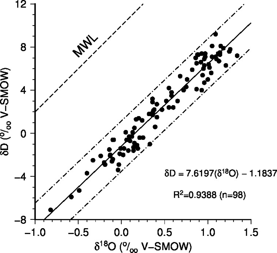
Following the well-established δD_sw and δ¹⁸O_sw linear relationship (Merlivat and Jouzel 1979), we found at the surface layer a moderate correlation (R²= 0.55, n=27), and at the intermediate and deeper layer, a stronger correlation (R²=0.94 and 0.81; n= 33 and 38, respectively). The δ¹⁸O_sw:δD_sw relationship for the whole dataset is presented in Figure 2 with a strong linear correlation (R²=0.94, n=98), which indicates that all of the future considerations regarding the δ¹⁸O_sw can be extrapolated to δD_sw including the Salinity and δ¹⁸O_sw relationship.

Because the slopes and intersection points for each of the layers were very similar (α=7.05, 7.02 and 6.91; b= -0.49, -0.67 and -1.4, respectively), we propose a mixing line gathering together the entire dataset (δD_sw= 7.62* δ¹⁸O_sw – 1.18) (Fig. 2). This mixing line has a slope very close to the Meteoric Water Line (MWL:α=8) (Craig 1961), which represents the average relationship between hydrogen and oxygen isotope ratios in natural waters.

Figure 2
The linear relation between δ¹⁸O_sw and δD_sw with three times the 95% confidence interval. The dashed line represents the Meteoric Water Line (MWL).

Following the Salinity and δ¹⁸O_sw relationship, the vertical δ¹⁸O_sw profile has a similar pattern to salinity (Fig. 3). The upper layer, corresponding to TW, is characterized by a maximum with values up to 1.34‰ and controlled mainly by the E-P balance (Craig and Gordon 1965). Along the SACW layer, there is a consistent depletion of this isotope from 1.13‰ at 180 m to 0.19‰ at 700 m. This behavior follows the temperature and salinity profile tendency in the thermocline. The δ¹⁸O_sw minimum is associated with the positioning of AAIW, which is characterized by minimum salinity derived from the sea melt and high precipitation rates in the Antarctic Divergence region (Tomczak and Godfrey 2003), which reduces the levels of δ¹⁸O_sw (up to -0.33‰). Below 1000 m depth, a slight increase of the δ¹⁸O_sw and salinity levels associated with the NADW layer can be observed.

Figure 3
- Vertical distribution of δ¹⁸O_sw (left), salinity (middle) and potential temperature (right) compared with Pierre and Ostlund. The solid and dashed line are the δ¹⁸O_sw vertical trend (3rd degree polynomial) for the present study and Pierre and Ostlund, respectively.

Still, in Fig. 3, the profile obtained in the present study has a large vertical variation that can be explained by the larger sample set (n=98 compared to the 68 and 24 measurements in Pierre and Ostlund, respectively), which provided a better resolution and consequently captured the natural environmental noise. Until 2000 m depth (the sampling limit of the present study), all three profiles are significantly aligned, which described a general and consistent vertical profile pattern for the South Atlantic Ocean.

As explained in the Oceanographic Settings, the bifurcation zone of the south and central branches of the SEC is located in the region between 5-14°S in the Winter. Additionally, the Intertropical Convergence Zone (ITCZ) is positioned in its northward position. Thus, it can be considered that during the present sampling period, there is no mesoscale process acting in the region and this consequently controls the physical isotopic fractionation. To verify the influence of the continental discharge on the isotopic content, the isotopic distribution was also analyzed in regard to the distance of the coast, and no pattern was clearly detected (Supplementary Material, Figure S1). This means that no evidence was found for the existence of a cross shelf fractionation pattern of the δ¹⁸O_sw and δD_sw in this region, probably due to a low contribution of river discharge.

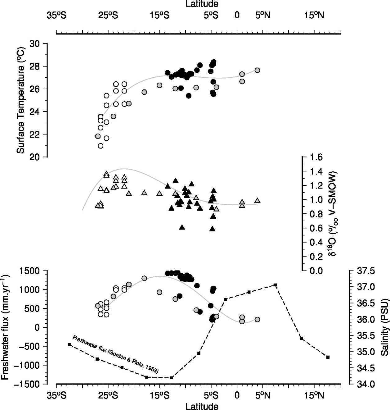
Because δ¹⁸O_sw and Salinity are strongly correlated and basically controlled by the same processes, a similar latitudinal behavior for these variables was expected, as suggested by Craig and Gordon (1965). However, the latitudinal distribution of the surface δ¹⁸O_sw and salinity for the Southwestern Tropical Atlantic (Fig. 4) showed that the salinity has a well-defined distribution with a maximum center near 15°S, corroborating the salinity budget proposed by Gordon and Piola (1983), whereas the δ¹⁸O_sw data revealed its highest levels near 25°S (Pierre et al. 1991).

Figure 4
Latitudinal distribution of surface temperature (top), δ¹⁸O_sw (middle), salinity (bottom) and freshwater flux (dashed line in the bottom; Gordon and Piola 1983). The black symbols represent the present data, the white ones represent Pierre et al. (1991), the grey are Ostlund et al. (1987) data and the lines are the general trends (4^th degree polynomial).

Previous studies of Pierre and Ostlund contributed to regional analysis of latitudinal fractionation, although hampered by the lack of regular spatial distribution. Nevertheless, combining the results of this work with these historical observations made it possible to validate the latitudinal separation of the Salinity and δ¹⁸O_sw relationship. As pointed out by Gordon and Piola (1983), northward the salinity maximum zone, the salinity and δ¹⁸O_sw have a similar decreasing tendency, which is most likely controlled by the high precipitation rates near the equator. However, south of 15°S, salinity has a strong increasing trend whereas the δ¹⁸O_sw levels are nearly stable (increase of 0.007‰ for each latitudinal degree). Fig. 5 shows the means and standard deviations of values δ¹⁸O_sw and Salinity for each water mass and considering only the samples with 60% or higher of a specific water mass. The seasonal fluctuation signal as a result of a δ¹⁸O_sw enrichment coupled to a freshwater input in the Southwestern Tropical Atlantic Ocean can be identified by the wide error bar in the TW salinity.

Figure 5
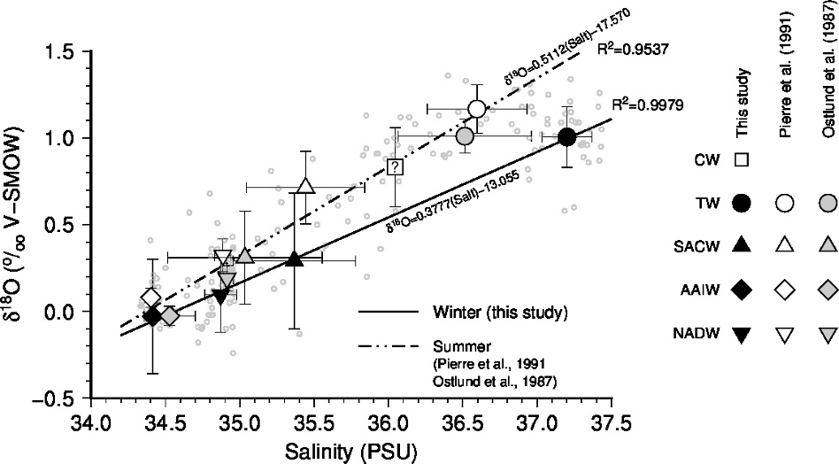
Means and standard deviation of salinity and δ¹⁸O_sw content for each water mass in the previous study in the Southwestern Atlantic Ocean – Pierre et al. (1991) (white symbols) and Ostlund et al. (1987) (grey symbols) and the present study (black symbols). The solid line represents the Winter Mixed Line and the dashed line represents the Summer Mixed Line. The raw data are presented as small grey dots.

DISCUSSION

Significant differences in salinity between ocean basins are apparent, especially the relatively higher salinities of the Atlantic Ocean. In part, this difference is due to the continental distribution in the ocean basins. The narrowing of the Atlantic contributes to higher evaporation rates, and consequently higher salinity values, since a large fraction of its surface area is influenced by continental dry air (Gordon et al. 2015). The δD:δ¹⁸O_sw relationship can be used as an indicator of the local E/P ratio, and δ¹⁸O_sw and salinity are also used for this purpose. Schmidt (1999) demonstrated that smaller slope in mixing lines are characteristic of evaporative areas (in opposite, regions with a high rainfall rate have steeper lines). However, most of the uncertainties surrounding the relationship between salinity and the stable isotopic composition of seawater are due to the lack of seawater isotope data (Conroy et al. 2014). The results of this study (93 new paired measures), when compared to the relationships obtained by Pierre and Ostlund, show differences in relation to the Winter (this study) and Summer (Pierre and Ostlund) line, reinforcing the argument of Schmidt (1999), considering the comparatively greater quantity of samples from this study. The weaker correlation in the surface, as shown in Fig. 2, can be an indicator that the hydrologic cycle (precipitation and evaporation) is not the only control in the δ¹⁸O_sw:δD_sw relationship for this region and other forcing (i.e., advection and lateral mixing) may have importance, as also found by Hasson et al. (2013) working in similar areas in the Pacific Ocean. Due to the different vapor pressure kinetic enrichment (fractionation factors) between δ¹⁸O_sw and δD_sw, evaporative regions have a smaller slope than the MWL (Craig and Gordon 1965, Gat 1996). Thus, the steepening can be used as an indicator of the local E/P ratio and the slope of 7.62 found here suggests that this region has a small evaporative tendency. Rohling (2007) analyzed 244 samples collected worldwide and proposed a similar equation (δD_sw= 7.37* δ¹⁸O_sw - 0.72). In both studies, the “deuterium excess” is slightly negative, which was already expected because it is relative to the average ocean water composition, referred to as the VSMOW (Rohling 2007, Kendall and Caldwell 1998).

This is an important tool because the use of δD_sw is gaining increasing attention in recent paleosalinity studies, considering that the combined use of the δ¹⁸O_sw and δD_sw measurements may reduce uncertainty and quantitatively improve the paleosalinity reconstructions (Conroy et al. 2014, Holloway et al. 2015). For example, Rohling (2007) proposed a new methodology for the combined use of δ¹⁸O_sw:δD_sw, restricting the impact of the hydrological cycle and thus characterizing changes in the surface water salinity, showing that paleosalinity reconstructions are possible with an uncertainty of 1 unit of practical salinity, especially in areas with high excess of deuterium values.

A clear separation regarding the salinity content of each water mass was observed in Fig. 5. However, the δ¹⁸O_sw did not show a distinct signature for each water mass because it is not possible to distinguish the water masses based only on their isotopic signatures. That isotopic signature masking can be attributed to the large distances between the study area and the sinking areas where those water masses were formed, which masked their initial isotopic characteristics. Despite the overlap in the standard deviations intervals, the current data have a widely scattered distribution if compared to the Pierre et al. (1991) and Ostlund et al. (1987) datasets, which suggests that in a regional scale the water masses do not have a homogeneous isotopic composition. Thus, the broader geographic distribution may reflect a natural larger dispersion of the isotopic data. Furthermore, the δ¹⁸O_sw average values obtained by Pierre and Ostlund were higher than in the present work, especially at the surface. This seems to be a response from a seasonal variation pattern. The probable cause for this shift in the Salinity and δ¹⁸O_sw relationship may be the intensification of the Brazil Current during the Summer season. An intensified BC would carry more Tropical Water to the subtropics and allow the occurrence of high δ¹⁸O_sw values in the first 200 m of the water column.

The lines representing δ¹⁸O_sw: Salinity in Fig. 5 get closer in layers with salinities near 34 and deviate in the high salinity layers, which is consistent with the seasonal differences in evaporation-precipitation budget and reinforced by the fact that the comparison datasets from Pierre and Ostlund are concentrated in austral Summer and this study in austral Winter. For example, a salinity of 37 (typical oceanic surface layer salinity) would have a difference of -0.43‰ between the Winter and Summer lines. However, for the layer of 35 psu, the difference becomes -0.16‰. This shows that the ratio is maintained in the deeper layers and has a larger variation in surface, which is most likely due to the evaporation and precipitation seasonal effects active in this layer.

The steeper slope of the Summer line indicates a negative E-P balance (Schmidt 1999), which should imply a δ¹⁸O_sw depletion (Meredith et al. 1999). However, as shown above, the Summer line (especially the surface section) has higher δ¹⁸O_sw levels than the Winter line, corroborating with the hypothesis that the increased volume of Tropical Water via Brazil Current may be responsible for the Summer δ¹⁸O_sw enrichment and the seasonal shift in the Salinity:δ¹⁸O_sw surface relationship. Additionally, the fact of the Coastal Water signature (collected in the Winter) falls exactly in the Summer line as an indication that this relationship is somehow influenced by the continental freshwater influx. Where excess freshwater intake is lowering salinity and stabilizing the upper ocean, mixing by mechanical turbulence is inhibited. Large enough freshwater inputs may lead to the formation of “barrier layers” in which a strong halocline inhibits the vertical exchange between the blend layer and the thermocline. Lukas and Lindstrom (1991) describe the barrier layer phenomena in the tropical Pacific, where the ITCZ is the source of fresh water. The tropical Atlantic also has barrier layers, where river discharge waters play a prominent role (Hu et al. 2004). The strong oceanographic component (advection) in the North Brazil Current (NBC), associated with the spatial and temporal variability of the ITCZ influence may contribute to the absence of isotope variation with the shoreline distance.

The δ¹⁸O_sw and salinity ratio varies temporally and spatially because all freshwater input to the ocean from precipitation and river inflow has a 0 psu whereas the δ¹⁸O_sw has distinct signatures at different latitudes (Bigg and Rohling 2000), and the freezing and melting processes distinctly influence these tracers (Tan and Strain 1980). This is one of the most controversial limitations of the paleosalinity residual estimative method, since it assumes the δ¹⁸O_sw and the salinity relationship remains constant through time and space (Toledo et al. 2007).

These spatial variations result in more reliable regional Salinity and δ¹⁸O_sw relationships (LeGrande and Schmidt 2006) instead of a Global Mixing Line because they can better represent the local interactions between these two variables. Additionally, and due to the lack of seawater isotopic data, efforts to understand the seasonal variation of this relationship are constrained to a few locations. We compared the present Salinity and δ¹⁸O_sw relationship against the Pierre and Ostlund data and the equation used by Toledo et al. (2007), as shown in Fig. 6.

Figure 6
The Southwestern Atlantic Mixing Line between δ¹⁸O_sw and salinity, and compared with Pierre et al. (1991), Ostlund et al. (1987) and Toledo et al. (2007). The dashed pointed line represents the averaged Mixing Line covering the seasonal fluctuations.

Based on the results found here, the seasonal variation of Salinity:δ¹⁸O_sw can generate paleosalinity uncertainties of 0.2 psu in the residual method estimate. The present dataset made it possible to compare the Salinity:δ¹⁸O_sw seasonally for the Southwestern Tropical Atlantic and the differences found are significant for the paleosalinity reconstructions, which opposes the idea that the South Atlantic would have a spatial and temporal constant Salinity and δ¹⁸O_sw relationship (Holloway et al. 2015).

Given the limitations of the current techniques to seasonally separate the samples for paleoceanographic studies, it seems more reasonable to use an averaged mixing line, which, in general, is intended to reduce errors in the paleosalinity estimations. In this regard, we propose SSS= 1.942* δ¹⁸O_sw + 34.56 as the Mixing Line to be used for future paleostudies in the Tropical South Atlantic Ocean. However, attention is needed regarding the paleosalinity estimation errors associated with the seasonal variations that were presented in this work.

CONCLUSIONS

The 93 new paired data points presented in this paper will help to improve the isotopic coverage for the South Atlantic. We found a strong correlation between δ¹⁸O_sw and δD that makes it possible to extrapolate the results for δ¹⁸O_sw to δD. Although it was not possible to distinguish the water masses based only on their isotopic signatures, the δ¹⁸O_sw vertical profile was proposed, which was also strongly associated with the salinity vertical distribution.

A difference in the Salinity and δ¹⁸O_sw relationship was found between 25°S and 5°N, which may be associated with seasonal changes in the transport of the western boundary currents (i.e. BC). This typical Summer and δ¹⁸O_sw contribution could be responsible for the seasonal Salinity:δ¹⁸O_sw variation, but more data are needed to confirm the role of the BC on the temporal variability of the Salinity and δ¹⁸O_sw relationship.

This paper has demonstrated that the δ¹⁸O_sw and salinity relationship for the Western Tropical South Atlantic has a seasonal variation pattern that might lead to paleosalinity differences of up to 0.2 psu between Summer and Winter. Considering the limitations of working with seasonal effects in the paleoceanographic studies, an intermediate Salinity:δ¹⁸O_sw Mixing Line for the Southwestern Atlantic was proposed to reduce the estimative errors associated with these seasonal fluctuations.

ACKNOWLEGMENTS

The data used in this work were collected by the Brazilian Navy Research Vessel Antares. The analysis was financially supported by the Geochemistry Network from PETROBRAS/CENPES and by the National Petroleum Agency (ANP) of Brazil (Grant 0050.004388.08.9) and by the Conselho Nacional de Desenvolvimento Científico e Tecnológico (CNPq). A.L.S Albuquerque and A.L. Belem are senior scholars from CNPq. Finally, we are grateful to the anonymous reviewers for their constructive comments that greatly contributed to improve the manuscript.

REFERENCES

• BENWAY HM and MIX AC. 2004. Oxygen isotopes, upper-ocean salinity, and precipitation sources. Earth Planet Sc Lett 224: 493-507.
• BERDEN G and ENGELN R. 2009. Cavity Ring-Down Spectroscopy: Techniques and Applications, Ed. Wiley, United Kingdom, doi: 10.1002/9781444308259.
• BIGG GR and ROHLING EJ. 2000. An oxygen isotope data set for marine waters. J. Geophys Res 105 C4: 8527-8536.
• CASTRO CG, PÉREZ FF, HOLLEY SE and RÍOS AF. 1998. Chemical characterization and modeling of water masses in the Northeast Atlantic. Prog Oceanogr 41: 249-279.
• CONROY JL, COBB KM, LYNCH-STIEGLITZ J and POLISSAR PJ. 2014. Constraints on the salinity–oxygen isotope relationship in the central tropical Pacific Ocean. Marine Chem 161: 26-33.
• CRAIG H. 1961. Isotopic variations in meteoric waters. Science 133: 1702.
• CRAIG H and GORDON LI. 1965. Deuterium and oxygen-18 variations in the ocean and the marine atmosphere. In: Tongiorgi E (Ed), Stable Isotopes in Oceanographic Studies and Paleotemperatures. Spoleto, Italy, p. 9-130.
• ELDERFIELD H and GANSSEN G. 2000. Past temperature and delta O-18 of surface ocean waters inferred from foraminiferal Mg/Ca ratios. Nature 405(6785): 442-445.
• ENGLEBRECHT AC and SACHS JP. 2005. Determination of sediment provenance at drift sites using hydrogen isotopes and unsaturation ratios in alkenones, Geochim Cosmochim Ac 69: 4253-4265.
• GAT JR. 1996. Oxygen and hydrogen isotopes in the hydrologic cycle. Annu Rev Earth Planet Sci 24: 225-262.
• GORDON AL, GIULIVI CF, BUSECKE J and BINGHAM FM. 2015. Differences among subtropical surface salinity patterns. Oceanogr 28(1): 32-39.
• GORDON AL and PIOLA AR. 1983. Atlantic Upper Layer Salinity Budget. J Phys Oceanogr 13: 1293-1300.
• HÄGGI C, CHIESSI CM and SCHEFUß E. 2015. Testing the D/H ratio of alkenones and palmitic acid as salinity proxies in the Amazon Plume. Biogeosci 12: 7239-7249.
• HASSON AE, DELCROIX T and DUSSIN R. 2013. An assessment of the mixed layer salinity budget in the tropical Pacific Ocean. Observations and modelling (1990–2009). Ocean Dynamics 63(2-3): 179-194.
• HOLLOWAY MD, SIME LC, SINAGARAYER JS, TINDALL JC and VALDES PJ. 2015. Reconstructing paleosalinity from δ18O: Coupled model simulations of the Last Glacial Maximum, Last Interglacial and Late Holocene. Quatern Sci Rev 131: 350-364.
• HU C, MONTGOMERY E, SCHMITT R and MULLER-KARGER F. 2004. The dispersal of the Amazon and Orinoco River water in the tropical Atlantic and Caribbean Sea: Observation from space and S-PALACE floats. Deep-Sea Research II, p. 51.
• HUT G. 1987. Consultants Group Meeting on Stable Isotopes Reference Samples for geochemical and hydrological investigations. Report to Director General. International Atomic Energy Agency, Vienna, 42 p.
• JOHNS W, LEE T, BEARDSLEY RC, CANDELA J, LIMEBURNER R and CASTRO B. 1998. Annual cycle and variability of the North Brazil Current. J Phys Oceanogr: 103-128.
• KENDALL C and CALDWELL EA. 1998. Fundamentals of Isotope Geochemistry. In: Kendall C and McDonnel JJ (Eds), Isotope Tracers in Catchment Hydrology. Elsevier Science B.V., Amsterdam, p. 51-86.
• KNOPPERS B, EKAU W and FIGUEIREDO AG. 1999. The coast and shelf of east and northeast Brazil and material transport. Geo-Marine Lett 19: 171.
• KROOPNICK PM. 1980. The distribution of 13C in the Atlantic Ocean. Earth Planet Sc Lett 49: 469-484.
• KROOPNICK PM. 1985. The distribution of 13C of ΣCO: in the world oceans. Deep-Sea Res 32: 57-84.
• LEGRANDE AN and SCHMIDT GA. 2006. Global gridded data set of the oxygen isotopic composition in seawater. Geophys Res Lett 33: L12604.
• LUKAS R and LINDSTROM E. 1991. The mixed layer of the western equatorial Pacific Ocean. J Geophys Res 96(S01): 3343-3357.
• MEREDITH MP, GROSE KE, MCDONAGH EL, HEYWOOD KJ, FREW RD and DENNIS PF. 1999. Distribution of oxygen isotopes in the water masses of Drake Passage and the South Atlantic. J Geophys Res Oceans (1978–2012) 104(C9): 20949-20962.
• MERLIVAT L and JOUZEL J. 1979. Global climatic interpretation of the deuterium-oxygen 18 relationship for precipitation. J Geophys Res 84: 5029-5033.
• MINOURA K, HOSHINO K, NAKAMURA T and WADA E. 1997. Late Pleistocene-Holocene paleoproductivity circulation in the Japan Sea: sea-level control on δ13C and δ15N records of sediment organic material. Palaeogeogr Palaeoclimatol Palaeoecol 135(1-4): 41-50.
• MULITZA S, BOLTOVSKOY D, DONNER B, MEGGERS H, PAUL A and WEFER G. 2003. Temperature: δ18O relationships of planktonic foraminifera collected from surface waters. Palaeogeogr Palaeoclimatol Palaeoecol 202: 143-152.
• NURHATI IS, COBB KM and DI LORENZO E. 2011. Decadal-scale SST and salinity variations in the central tropical Pacific: signatures of natural and anthropogenic climate change. J Clim 24 (13): 3294-3308.
• OSTLUND HG, CRAIG H, BROECKER WS and SPENCER D. 1987. GEOSECS Atlantic, Pacific and Indian ocean expeditions, shorebased data and graphics, Vol. 7. Technical report, I.D.O.E. National Science Foundation, p. 200.
• PHILANDER SGH, GU D, LAMBERT G, LI T, HALPERN D, LAU NC and PACANOWSKI RC. 1996. Why the ITCZ is mostly north of the equator. J Clim 9: 2958-2972.
• PICKARD GL and EMERY WJ. 1990. Descriptive Physical Oceanography. An Introduction. 5th ed., Butterworth-Heinemann Ltd. Great Britain. doi: 10.1029/CE051p0036.
• PIERRE C. 1999. The oxygen and carbon isotope distribution in the Mediterranean water masses. Marine Geol 153: 41-55.
• PIERRE C, VERGNAUD-GRAZZINI C and FAUGÈRES JC. 1991. Oxygen and carbon stable isotope tracers of the water masses in the Central Brazil Basin. Deep-Sea Res 38(5): 597-606.
• REDFIELD AC and FRIEDMAN I. 1965. Factors affecting the distribution of deuterium in the ocean. In Symposium on Marine Geochemistry. Rhode Island University Narragansett Marine Laboratory Occasional Publication, Vol. 3, p. 149-168.
• ROHLING EJ. 2007. Progress in paleosalinity: Overview and presentation of a new approach. Paleoceanogr 22(3). DOI: 10.1029/2007PA001437.
• SCHMIDT GA. 1999. Error analysis of paleosalinity reconstructions. Paleoceanogr 14(3): 422-429.
• SCHMIDT GA, BIGG GR and ROHLING EJ. 1999. Global Seawater Oxygen-18 Database - v1.21. http://data.giss.nasa.gov/o18data/
  » http://data.giss.nasa.gov/o18data/
• SCHNEIDER T, BISCHOFF T and HAUG GH. 2014. Migrations and dynamics of the intertropical convergence zone. Nature 513: 45-53.
• SCHOTT F, FISCHER J and STRAMMA L. 1998. Transports and pathways of the upper-layer circulation in the western tropical Atlantic. J Phys Oceanogr 28: 1904-1928.
• SCHOUTEN S, OSSEBAR J, SHREIBER K, KIENHUIS MVM, BENTHIEN A and BIJMA J. 2006. The effect of temperature, salinity and growth rate on the stable hydrogen isotopic composition of long chain alkenones produced by Emiliania huxleyi and Gephyrocapsa oceanica. Biogeosci 3: 113-119.
• STRAMMA L, FISCHER J and REPPIN J. 1995. The North Brazil Undercurrent. Deep Sea Res Part I 42: 773-795.
• STRAMMA L and ENGLAND M. 1999. On the water masses and mean circulation of the South Atlantic Ocean. J Geophys Res 104(C9): 20863-20883.
• TAN FC and STRAIN PM. 1980. The distribution of sea ice meltwater in the eastern Canadian Arctic. J Geophys Res Oceans (1978–2012) 85(C4): 1925-1932.
• THORNALLEY DJR, ELDERFIELD H and MCCAVE IN. 2010. Intermediate and deep water paleoceanography of the northern North Atlantic over the past 21,000 years. Paleoceanogr 25: PA1211.
• TOLEDO FAL, COSTA KB and PÍVEL MAG. 2007. Salinity changes in the western tropical South Atlantic during the last 30 kyr. Global Planet Change 57: 383-395.
• TOMCZAK M and GODFREY JS. 2003. Regional Oceanography: an introduction. 2nd ed., Cap. 6, p. 63-82.
• VENÂNCIO IM, BELEM AL, SANTOS THR, ZUCCHI MR, AZEVEDO AE, CAPILLA R and ALBUQUERQUE ALS. 2014. Influence of continental shelf processes in the water mass balance and productivity from stable isotope data on the Southeastern Brazilian coast. J Marine Syst 139: 241-247.
• WAELBROECK C, LABEYRIE L, MICHEL E, DUPLESSY JC, MCMANUS JF, LAMBECK K, BALBON E and LABRACHERIE M. 2002. Sea-level and deep water temperature changes derived from benthic foraminifera isotopic records. Quatern Sci Rev 21: 295-305.

Publication Dates

• Publication in this collection
  30 Sept 2019
• Date of issue
  2019

History

• Received
  3 Mar 2018
• Accepted
  9 Dec 2018