Abstract
Abstract: This study deals with the subject biomass estimation. The objective was to achieve the additivity of tree biomass components, which is defined as the compatibility among the component predictions and total tree biomass, using ratio estimates. The biomass estimation model was applied to black wattle trees in forest stands, which include a sample of 670 trees in an age range of 1 to 10.75 years. The adjusted model, in which the total biomass, or sum of predicted components, is a function of the stem volume multiplied by the Scalar Coefficients Proxy of Density, proved to be of great interest for biomass estimation and consistent when compared to the results obtained by WNSUR estimates (traditional method). The natural additivity of the tree biomass components was fully achieved, when modeling them by means of ratio estimation. Equations developed from the proportional behavior of the biomass components at different ages did not require the use of linear regression models and were obtained from calibration with the experimental data. The estimators resulting from these equations proved to be appropriate to make a generic model for correction of ratios coefficients at different ages.
Key words
scalar coefficients proxy of density; ratio estimate; stem volume; quadratic mean diameter; WNSUR
INTRODUCTION
Biomass in native and planted forests has been increasingly estimated for several purposes in Brazil, highlighting the diverse demands in the energy context, for the assessment of carbon neutralization and to deepen the understanding of the dynamic processes that occur in forest ecosystems over a productive cycle.
Worldwide two schools have contributed substantially to the improvement of biomass modeling in trees. The first one has been working to overcome the innumerable screenings resulting from the incompatibility of additivity and acceptable precision resulting from the systems of equations adjusted by means of linear and nonlinear regressions.
The second one evolved trying to overcome also the problems of precision of the estimates obtained for each of the components of the trees by means of segmented modeling, that is, trying to improve consistent methodologies to have the best geometric volume of the components, a consistent model to correct shape of these volumes and a model for obtaining density of each component to generate their respective biomasses.
This study deals with the subject biomass estimation which is an indirect goal in the forest inventories and ensures, in essence, the reduction of costs by avoiding the direct measurement of the mass of all trees.
It is a fact that researchers usually apply volume models to biomass estimation. Because biometric variables taken from trees, either isolated or combined, do not have the same metric unit as the dependent variable; this type of modeling becomes very complex. The aim of this work is precisely to address this important issue, making an assumption before defining the model, either using regression or segmented modeling to estimate biomass in a forest area: The metric units of independent variables in a model must be composed to keep the same metric unit of the dependent variable.
If we strictly hold to this assumption, we can easily deduce that the variables d (stem diameter at breast height) and h (tree height), as they are used in the volumetric models, alone or combined, do not present metric units compatible with the dependent variable for biomass estimation, which should be expressed in kg.
A second assumption must also be considered in the modeling of biomass: the additivity, which corresponds to the compatibility among tree component estimates (leaves, branches, bark, stem and root), i.e., the sum of the masses of the components must be equal to the total tree mass.
Although biological diversity is surprising and complex, many of the fundamental biological processes manifest themselves in an extraordinarily simple way when equated according to their size, independent of the class or taxonomic group they belong to (West and Brown 2005WEST GB AND BROWN JH. 2005. The origin of allometric scaling laws in biology from genomes to ecosystems: towards a quantitative unifying theory of biological structure and organization. J Exp Biol 208: 1575-1592.). This scaling, according to Niklas (1994)NIKLAS KJ. 1994. Plant allometry: the scaling of form and process. Chicago: University of Chicago Press, 412 p., follows a power-law behavior, as defined in (1).
Where: Y= some quantifiable biological variable; α = normalization constant; X= mass of the organism; β = scale exponent.
An additional simplification can be achieved, since the exponent β assumes a limited set of values, which are typically simple multiples of 1/4 (West et al. 1999WEST GB, BROWN JH AND ENQUIST BJ. 1999. The fourth dimension of life: fractal geometry and allometric scaling of organisms. Science 284: 167-169.). Many biological variables follow this scale as they were presented and discussed by West et al. (1997WEST GB, BROWN JH AND ENQUIST BJ. 1997. A general model for the origin of allometry scaling laws in biology. Science 276: 122-126., 1999), Enquist et al. (1998ENQUIST BJ, WEST JH AND WEST GB. 1998. Allometric scaling of plant energetics and population density. Nature 395: 163-165., 1999ENQUIST BJ, WEST GB, CHARNOV EL AND BROWN JH. 1999. Allometric scaling of production and life-history variation in vascular plants. Nature 401: 907-911.), Enquist and Niklas (2001)ENQUIST BJ AND NIKLAS KJ. 2001. Invariant scaling relations across tree-dominated communities. Nature 410: 655-660., Enquist (2002)ENQUIST BJ. 2002. Universal scaling in tree and vascular plant allometry: toward a general quantitative theory linking plant form and function from cells to ecosystems. Tree Physiol 22: 1045-1064., Niklas (2004)NIKLAS KJ. 2004. Plant allometry: is there a grand unifying theory? Biol Rev 79: 871-889. and West and Brown (2005).
The theme allometry was consolidated by Huxley (1932)HUXLEY JS. 1932. Problems of relative growth. London: Methuen & Co., Ltd., 276 p., who synthesized the theoretical conception about growth and its scales. He assumed that the growth rate of an organ was simultaneously proportional to a constant characteristic of the organ itself (ξ), given its size at the time , and to a general factor, common to all parts of the organism, representing the effects of its age and of the environmental conditions . Taking the size of the organism as Y with constant feature η, the specific growth rates of organs and of the organism may be defined in (2), with solution of the derivatives in (3).
The expression defined in (3) has solution in (4) and (5), explaining the origin of the model presented in (1).
Considering (C2 - C1) = log α, then:
Recomposing the function on its original form we have:
Allometry is also associated to properties of such changes in the organism, whose characteristics are related to its size. Thus, Niklas (2004) also defines allometry as the study of size and its consequences, according to the model presented in (6), in which Y is the size of the body’s component (measured by its size or mass), X is a comparable measure of the body’s size, excluding the size of the body part of interest, α is the allometric constant and β the allometric exponent (scale).
In Forest Science, the model presented in (6) is one of the most common allometric forms (Chan et al. 2013CHAN N, TAKEDA S, SUZUKI R AND YAMAMOTO S. 2013. Establishment of allometric models and estimation of biomass recovery of swidden cultivation fallows in mixed deciduous forests of the Bago Mountains, Myanmar. For Ecol Manage 304: 427-436.). Although it is a simple allometric model, it has been widely used to estimate the biomass components stem volume and height of the trees, especially considering the variable diameter at breast height (d) as a predictor.
The most appropriate method to evaluate the biomass of a tree is to obtain it separately for each component, implying in its cutting and resulting in a time-consuming task and high cost. An alternative approach is to employ allometric equations, i.e., trees biometrically measured are converted into biomass values by means of empirical allometric models (Brown 1997BROWN S. 1997. Estimating biomass and biomass change of tropical forests: a primer. FAO Forestry Paper 134.). There is a vast literature regarding the development and use of allometric biomass models, which was revised by Picard et al. (2012)PICARD N, SAINT-ANDRÉ L AND HENRY M. 2012. Manual for building tree volume and biomass allometric equations: from field measurement to prediction. Food and Agricultural Organization of the Unites Nations and Centre de Coopération Internationale en Recherche Agronomique pour le Développement, Rome and Montpellier, 215 p..
Thus, the allometry in the context of the estimation of tree biomass refers to mathematical equations related to the components and total biomass based on characteristics that are easily measured such as diameter at breast height (d), height of the tree (h), wood density (ρ), and crown diameter (Dc). It is obvious that the equations must be based on destructive sampling and then applied generically (Chave et al. 2014CHAVE J ET AL. 2014. Improved allometric models to estimate the aboveground biomass of tropical trees. Glob Chang Biol 20: 3177-3190.), and the quality of these allometric models constitutes one of the most important limitations in the assessment of biomass stocks (Chave et al. 2004CHAVE J, CONDIT R, AGUILAR S, HERNANDEZ A, LAO S AND PEREZ R. 2004. Error propagation and scaling for tropical forest biomass estimates. Philos Trans R Soc B 359: 409-420., Sanquetta et al. 2015SANQUETTA CR, WOJCIECHOWSKI J, CORTE APD, BEHLING A, PÉLLICO NETTO S, RODRIGUES AL AND SANQUETTA MI. 2015. Comparison of data mining and allometric model in estimation of tree biomass. BMC Bioinformatics 16(247): 1-9.).
The objective of this work is to establish a simple and consistent biological model, testing its performance statistically precise, which estimates biomass accurately. Our proposal was conceived by deriving a new segmented model. Ratio estimator’s performance was compared with those obtained by regression modeling via SUR and NSUR methodologies. Application of other segmented models to the present data set was not possible because they were not collected to attain all the required information to perform the estimates.
The goal of this research is to develop a segmented model based on the following hypothesis: “The biomass performed by a simple model, using ratio estimates, does not require additional methodological stratagem to attain additivity and achieving competitive precisions with those obtained by the regression models”.
MATERIALS AND METHODS
APPROACHES FOR BIOMASS MODELING
Estimation using regression modeling
When the model in (6) is adjusted using empirical data, both biomass and predictor variables often faces heteroscedasticity of errors, i.e., a condition in which the variance of errors is not constant. This directly affects the estimator, because when (6) is linearized and the ordinary least squares is applied to estimate the parameters, the estimator does not ensure the smallest variance, i.e., ceases to be unbiased (the best linear unbiased estimator - BLUE). This will introduce bias in the conclusions drawn from the results of the significance tests of the equations and confidence intervals for the coefficients and for the estimates of mean biomasses and their prediction.
Parresol (1999)PARRESOL BR. 1999. Assessing tree and stand biomass: a review with examples and critical comparisons. Forest Sci 45: 573-593. demonstrated that the heteroscedasticity of errors can be explained by the modeling - which follows a normal distribution with increasing variance as a function of , expressed by an exponential relation of , allowing the establishment of weights. Thus, the model (6) can be adjusted by generalized least squares, resulting in a BLUE estimator and, consequently, validating the tests of significance of the equation and the construction of confidence intervals. This method has been preferable, because there is no need to transform the parameters estimates of the model.
Considering the theory of allometric partition (TAP), it can be affirmed that the separation of plants into components is regulated mainly by their total size, but keeps a scale relationship between these parts and the whole (West et al. 1999, Savage et al. 2008SAVAGE VM, DEEDS EJ AND FONTANA W. 2008. Sizing up allometric scaling theory. PLoS Comput Biol 4: 17.). West et al. (2000)WEST GB, BROWN JH AND ENQUIST BJ. 2000. The origin of universal scaling laws in biology. In Scaling in Biology [Brown JH and West GW (Eds)], p. 87-112. New York: Oxford University Press. presented a model in which they sought to provide a theoretical basis for allometric relationships in trees, considering the model presented in (1). The objective was to clarify an explanatory theory for the empirical relationships between the characteristics of vascular plants and not just to observe them. The model is based on principles of hydrodynamics, biomechanics, and tree architecture and provides many scales multiple of 1/4 for various attributes of the tree, which are presented in Enquist (2002).
According to Ducey (2012)DUCEY MJ. 2012. Evergreenness and wood density predict height–diameter scaling in trees of the northeastern United States. For Ecol Manage 279: 21-26., generality is often not observed and this has led to questions as to how the allometric scales relations are apparently variant for species and between large spatial domains, especially when applied to tree biomass equations. Niklas (1995)NIKLAS KJ. 1995. Size-dependent allometry of tree height, diameter and trunk-taper. Ann Bot 75: 217-227. has shown that the allometric relationships change within the same individual throughout its life and in the growth conditions to which it is subjected to, and also referred to this size-dependent allometry as evidence that no universal allometric scaling coefficients could be estimated for trees.
Although it is common to use the model (6), Jenkins et al. (2003)JENKINS JC, CHOJNACKY DC, HEATH LS AND BIRDSEY RA. 2003. National-scale biomass estimators for United States tree species. Forest Sci 49: 12-35. and Weiskittel et al. (2015)WEISKITTEL AR, MACFARLANE DW, RADTKE PJ, AFFLECK DLR, TEMESGEN H, WOODALL CW, WESTFALL JA AND COULSTON JW. 2015. A Call to Improve Methods for Estimating Tree Biomass for Regional and National Assessments. J For 113(4): 414-424. point out that there are substantial evidences that the diameter (d) can often be a poor variable to estimate the biomass of the components. This is also referenced by Goodman et al. (2014)GOODMAN RC, PHILLIPS OL AND BAKER TR. 2014. The importance of crown dimensions to improve tropical tree biomass estimates. Ecol Appl 24(4): 680-698., when they demonstrated that trees with disproportionate crown diameters may have a relationship between d and total biomass different from trees with proportional crown diameter.
Chave et al. (2009)CHAVE J, COOMES D, JANSEN S, LEWIS SL, SWENSON NG AND ZANNE AE. 2009. Towards a worldwide wood economics spectrum. Ecol Lett 12: 351-366. also showed a high degree of variability in the relationship between tree size and wood density, thus reinforcing that simple dimensional measurements may be insufficient to obtain accurate estimates of tree biomass due to the variability of wood density. According to MacFarlane (2015)MACFARLANE DW. 2015. A generalized tree component biomass model derived from principles of variable Allometry. For Ecol Manage 354: 43-55., these important differences are related to the dimensioning between the parts relative to the whole, known as allometry.
Brown et al. (2004)BROWN JH, GILLOOLY JF, ALLEN AP, SAVAGE VM AND WEST G. 2004. Toward a metabolic theory of ecology. Ecology 85(7): 1771-1789. noted that the power-law model allowed the definition of other models for allometric scaling in biology. Therefore, the basic form of the model in (6) can be extended to other forms. Instead of using to represent the value of only one feature, it can be extended to represent values of more than one feature, for example, for biomass: d,h and .
In Europe, a comprehensive review on biomass equations was performed by Zianis et al. (2005)ZIANIS D, MUUKKONEN P, MÄKIPÄÄ R AND MENCUCCINI M. 2005. Biomass and stem volume equations for tree species in Europe. Silva Fenn, 63 p., in which they reported a total of 607 equations adjusted for 39 species distributed in all European countries. This review highlights that the vast majority of researches (127) used the model log (M) = A + B log (D), however the volumetric models of Schumacher and Hall (1933)SCHUMACHER FX AND HALL FS. 1933. Logarithmic expression of timber-tree volume. J Agric Res 47(9): 719-734. and Spurr (1952)SPURR SH. 1952. Forest inventory. New York: The Ronald Press Company, 476 p., and their variations, were prevalent in other citations.
Ketterings et al. (2001)KETTERINGS QM, COE R, VAN NOORDWIJK M, AMBAGAU Y AND PALM CA. 2001. Reducing uncertainty in the use of allometric biomass equations for predicting aboveground tree biomass in mixed secondary forests. For Ecol Manage 146: 199-209. showed how the function in (6), making X=d, could be generalized to refer explicitly to tree height (h) and wood density . Assuming that the biomass Y is initially considered only as a function of the diameter d, then , in which the coefficients a and b vary between sites. This variation is probably the major source of uncertainty if the biomass estimations are obtained using equations that are not calibrated for different sites. However, if the calibration is performed by collecting biomass data B and diameters d for each site, this procedure is costly and requires destructive actions. Methods to obtain the values of a and b must, therefore, be proposed such that destructive procedures are not required. The parameter b can be estimated by means of a specific relationship of the site between tree height h and diameter d, i.e., . The parameter a may be estimated from the average of wood density ρ in the site as , where r is a constant relatively stable among sites. As biomass is proportional to , then they have assumed that . There is a critical point in this model when they considered the constant r to be relatively stable among sites, because the site variations have been not satisfactorily treated in most of the biomass models, owing to their complexity.
The model presented in (6) was also enhanced by MacFarlane (2015), which applied it to a system of specific equations for the proposed components. Considering what was explained by Ketterings et al. (2001), we can maintain the form associated with equation (6), expressing it in a generalized way and with a more consistent biological meaning to estimate biomass of the tree components.
Where: Y= biomass of the tree above the ground (kg); d= diameter at breast height (cm); h= height of the tree (m); ρ = wood density (kg.m-3, measured in d); F= form factor of the whole-tree- defined by Gray (1966)GRAY HR. 1966. Principles of forest tree and crop volume growth: a mensuration monograph. National Development, Forestry and Timber Bureau, Canberra, 54 p. and Cannell (1984)CANNELL MGR. 1984. Woody biomass of forest stands. For Ecol Manage 8: 299-312. for indexing the tree biomass, relative to the proxy mass, which is a proxy of the tree volume multiplied by the density of the tree, i.e. , which he termed proxy biomass of the tree.
Thus, MacFarlane (2015), in view of the possibility of no proportionality between the biomass of the components and the proxy biomass of the tree, proposed the solution presented in (8), in which, when B ≠ 1, the relationship does not keep proportionality, indicating that the form changes when the tree biomass changes:
In this way, he proposes the preliminary segmentation for B= 1 in the equation (8), for each of the components of the tree, formalizing them as are presented in (9), (10) and (11):
Where: Y1, Y2 and Y3 are respectively the biomass of the neiloide, considered to a height of 1.30m (HB); of the commercial stem, considered from 1.30m of the tree until the beginning of the crown (HC- HB) and of the living crown, considered the beginning of the first branch alive until the top of the tree (H - HC).
He also proposed a further separation of the crown biomass, wherein there is a dominant central segment which is separated from its other branches. The mass of these other branches is associated with a differentiated form factor, which he named as abstract form factor (F4) and is applied to an equally abstract volume of this component, calculated by . W is the average crown width which, when multiplied by its density, will result in the biomass of this component , and is named as Y4, such that . Consequently, the total biomass of the tree is obtained by the sum of these components, i.e.: .
When the occurrence of non-proportionality is detected in the form component, as is shown in (8), we can experimentally identify the respective values of the coefficient B for each of the components, i.e., B1, B2, B3 and B4. This system of equations was solved using the Seemingly Unrelated Regression (SUR) model.
However, given the difficulty of obtaining the volume of components vj experimentally in the sampled population, researchers have proposed to apply regression models to identify the biomass of the components using biometric variables more accessible in the forest, leading, as a consequence, to the loss of additivity or the use of the segmented models previously presented in (8), (9), (10), and (11). The concept of additivity of the biomass components was developed from the 1970s, when several researchers (Kozak 1970KOZAK A. 1970. Methods of ensuring additivity of biomass components by regression analysis. For Chron 46(5): 402-404., Chiyenda and Kozak 1984CHIYENDA SS AND KOZAK A. 1984. Additivity of component biomass regression equations when the underlying model is linear. Can J For Res 14: 441-446., Cunia and Briggs 1984CUNIA T AND BRIGGS RD. 1984. Forcing additivity of biomass tables-add empirical results. Can J For Res 14: 376-384., 1985CUNIA T AND BRIGGS RD. 1985. Forcing additivity of biomass tables: use of the generalized least squares method. Can J For Res 15: 23-28., Reed and Green 1985REED D AND GREEN EJ. 1985. A method of forcing additivity of biomass tables when using nonlinear models. Can J For Res 15: 1184-1187.) began to formulate methods to compose the biomass equations in order to force them to additivity. In this condition, the two variables, form factor F and wood density ρj are associated to the coefficients of the proposed regression models, but without configuring a balanced participation in each of them when adjusted for the components, which generates loss of additivity.
Some assumptions need to be defined to ensure accuracy in the prediction of forest biomass on a large scale. Genet et al. (2011)GENET A ET AL.. 2011. Ontogeny partly explains the apparent heterogeneity of published biomass equations for Fagus sylvatica in central Europe. For Ecol Manage 261: 1188-1202. state that a good set of equations for this purpose must meet the following characteristics: i) consistency - referring to the separation of the tree total biomass in standard components, however, ensuring its additivity, ii) robustness - referring to the composition of an operating system that works correctly for wide variations in the sample population and with low sensitivity to the used sampling procedure and to the formulated hypothesis, and (iii) accuracy.
According to Genet et al. (2011), many recent studies with tropical and temperate species have dealt with the variations of allometric parameters and their relationships (Chave et al. 2005CHAVE J ET AL. 2005. Tree allometry and improved estimation of carbon stocks and balance in tropical forests. Oecologia 145: 87-99., Saint-Andre et al. 2005SAINT-ANDRE L, M’BOU AT, MABIALA A, MOUVONDY W, JOURDAN C, ROUPSARD O, DELEPORTE P, HAMEL O AND NOUVELLON Y. 2005. Age-related equations for above- and below-ground biomass of Eucalyptus hybrid in Congo. For Ecol Manage 205: 199-214., António et al. 2007ANTÓNIO N, TOMÉ M, TOMÉ J, SOARES P AND FONTES L. 2007. Effect of tree, stand, and site variables on the allometry of Eucalyptus globulus tree biomass. Can J For Res 37: 895-906., Wutzler et al. 2008WUTZLER T, WIRTH C AND SCHUMACHER J. 2008. Generic biomass functions for Common beech (Fagus sylvatica) in Central Europe: predictions and components of uncertainty Can J For Res 38: 1661-1675., Pretzsch 2009PRETZSCH H. 2009. Forest Dynamics, Growth and Yield. Berlin: Springer, 664 p.). They highlighted that both the allometric factor and the allometric exponent vary between stands of different ages, different levels of fertility and between species. However, there is still no consensus on how to appropriately treat these effects.
Zianis and Mencuccini (2004)ZIANIS D AND MENCUCCINI M. 2004. On simplifying allometric analyses of biomass. For Ecol Manage 187: 311-332. consider the model presented in (1) as the most common for biomass studies (M). It takes the diameter measured at 1.30m (D) to express the variable X and, after having been linearized, results in:
They explained the behavior of the coefficients a and b by taking advantage of the fractal geometry and the size and form of the trees. These procedures allow them to adjust statistical functions for these coefficients based on the relations:
i) If the tree volume is proportional to diameter times height, and height is proportional to diameter, they have:
Then:
Consequently,
Under these conditions, b can be estimated by
Where: b* varies between 0 < b* ≤ 1, obtained experimentally for different species using the relationship presented in (14) and (16).
The coefficient “a” can be estimated as a function of b.
Estimation using segmented models
Vallet et al. (2006)VALLET P, DHOTE JF, MOGUEDEC GL, RAVART M AND PIGNARD G. 2006. Development of total aboveground volume equations for seven important forest tree species in France. For Ecol Manage 229: 98-110. introduced a new concept to treat biomass and carbon estimators in trees when they worked with the segmented models, that is, each parameter of the model is estimated separately. This approach avoids the problems generated by the regression-adjusted models, in which the parameters form and density integrate all other coefficients and cause loss of the additivity. Consequently, the consistency of the model is reduced, not meeting the first characteristic formalized by Genet et al. (2011). Vallet et al. (2006) proposed a model to estimate the total amount of carbon per tree C, as it is shown in (19):
Where: C= total carbon per tree; VIFN = commercial volume; BRANCHEF= expansion factor for the branches’ volumes; DEN= basic density for the species and CAR= carbon proportion in dry matter.
To avoid the use of an expansion factor to the branches, the total volume for the entire tree, including the branches, was considered as it is presented in (20):
Consequently,
Please, note that still remains the estimator for F, as shown in (20), that the author proposes to be equated in (22):
To avoid the correlation between C130 and htot, the variable hardiness of the tree (hdn) was proposed and equated in (23):
Note that the higher the value of hdn more robust is the tree and the lower this value is, slenderer it will be. By replacing (22) in (20) they have:
The total variance of the estimator can be obtained in (25):
Where: σ= variance of the residuals and , are respectively the variances and covariance of the variables.
Genet et al. (2011) proposed the allometric model in (26):
Where: DM= dry mass for certain component; d= diameter taken at 1.30m; h= total height; α , β and γ = model parameters to be estimated and ε = error attributed to the not explained variability.
As the tree biomass results from the characteristics: volume, wood density and form, the scalar value β represents the product of the form factor F by the wood density ρ, i.e., . The form factor was calculated using the estimator proposed by Vallet et al. (2006), as it is shown in (22).
Vallet et al. (2006) also took the pre-existing biomass equation for the species Beech, in Europe, i.e., (d in m and d2h in m3) and calibrated it to be adapted to the model in (27). Considering the constant c ≠ 0 , the calibration was applied to the sample data from France and equated the variable d in such a way as to make it equal to d2h in the equation, with the following function:
Genet et al. (2011) found, calibrating the equation (27), the following values for k and q: k = 60.5 q = 0.368 for d < 0.25 m, and k = 34.7 q = 0.439 for d ≥ 0.25 m.
Therefore, they have in the biomass model:
They also proposed to adjust the biomass estimate as a function of age (A) and obtained their final models in (29) for the tree components and in (30) to the total biomass above ground:
In the present work, we will maintain the same concept of the previously mentioned authors, that is, the use of the segmented model, and we will introduce a new concept for the additivity of the tree components, which is the compatibility of the biomass estimates of the components with the total stem biomass without using any method to force it, as it occurs in these variables naturally. In addition, it differs from methods that force the additivity, because each biomass component and the total biomass are represented by their own equations. The biomass additivity, as proposed in this work, will only be achieved when using a model as simple as possible: linear and of first order, i.e., . The application of models of other orders requires the transformation of the data and this leads to loss of additivity, i.e., there is an incompatibility of the biomass component estimates relative to the total biomass.
CONCEPTION FOR BIOMASS MODELING IN THIS RESEARCH
Consider first the theoretical conception presented by MacFarlane (2015) in (7), then proceed as follows.
Form factor (F)
The first phase of this design will be to propose a facilitating solution concerning the form factor (F) to make the biomass estimation model operationally less complex.
Consider the methodology proposed by Hohenadl (1924)HOHENADL W. 1924. Der aufbau der baumschafte. Forstwiss Cbl 44: 17-18. (as cited in Prodan 1965), which divides the tree stem in five or more parts of equal length. However, according to Prodan (1965)PRODAN M. 1965. Holzmesslehre. Sauerlanger’s Verlag, Frankfurt am Main., the smaller the length of the segments, the closer the volume estimate is to the real value. Thus, dividing the bole of the tree in ten segments, whose length is proportional to the total tree height, will increase the accuracy of these estimates (Figure 1).

To obtain the relationship between the natural and artificial form factor, Ko (1968)KO YZ. 1968. Beziehungen zwischen formquotienten und formzadl. Doctoral thesis, Albert Ludwigs University. introduced the following concept on the quadratic diameter ( ), considering the natural form factor calculated by the Hohenadl’s method:
Where: the mean quadratic diameter of the series can be obtained inside the parentheses, i.e.:
The Hohenadl’s natural form factor () will be then obtained as:
This concept of form factor was enlarged by Ko (1968) using the expression (34), in which the diameter taken at any relative height of the series is considered as the reference to obtain any natural desired form factor:
Where: dx = reference diameter and d0.i = measured diameters in the middle of each segment.
Taking the mean quadratic diameter as reference, we get the form factor equal to one (Prodan 1965).
The form of the tree, in this case, is equivalent to a cylinder whose diameter is coincident with the mean quadratic diameter. Consequently, the volume is obtained in (36):
Using the form factor equal to one in (36), there is a simplification to obtain the volume of the cylinder Vs equivalent to the stem volume, whose reference is in dq:
Additivity of biomass components
Equating the relationship of the various biomass estimates of the tree components with the cylinder volume in (37) will make this estimator a ratio with specific meaning, constituting the central objective of this work.
Consider that the variable biomass of the components will be called Yij, such that j indicates the component to which the estimator i refers, i.e., it will be equal to c if the estimator is for the crown of the tree; equal to s if the estimator is for the stem; b for the bark; r for root and t for the total. The volume of each component will be called Xij in much the same way as if configured for the variable Yij, which will allow the specification of the following model:
- i)Theorem 1: Additivity of components
-
If the biomass components of a tree are obtained by the product of scalars of their densities equated as a function of the stem volume, then the sum of the resulting biomass will be equal to the biomass of the whole.
- ii)Proof
-
Let Yj denote the biomass of the components of a tree,
their densities and vj the volume of their respective components, such that j = 1, 2, 3 .... k components, then:
Consequently, if we take the volume of each component multiplied by its density, we will obtain the respective biomass and the results of these estimates are additives.
However, given the difficulty of obtaining the experimental volumes of the components vj, except for the stem volume vs, which is the easiest component to be obtained, and in the present case will be calculated as defined in (37), then dividing all the terms of the equality in (39) by this estimator we have:
If the proportions are denominated , then the densities of the components are multiplied by a weight that expresses proportions of the stem volume. Rewriting the equation in (40) we have:
Note that = Rj , which expresses exactly the ratio between the biomass components and the stem volume , then such ratios are called Scalar Coefficients Proxy of Density - SCPD, which will be the actual density only in the case of the stem biomass estimator. Consequently,
As observed, if the denominator vs is constant for all components, then the equation (42) can be rewritten as in (43).
As a consequence, the obtaining of these ratios experimentally per component in each tree in the forest, as a function of the stem volume, continues to be additive, because SCPDs are proportions of this volume. This completes the proof.
iii) Corollary 1: Additivity for a sample
If a sample of size n is taken from a forest population, such that the sample size sufficiency is ensured, then the biomass of the components of the n sampled trees can be added and their respective means can be obtained.
Consequently,
As can be noted, the additivity of the biomass means, for a sample of n trees obtained by means of ratio estimates still holds.
Consequently, in the segmented models, it is also possible to establish a sample structure to directly obtain estimates of the tree component basic density using fitted models as a function of the variables diameter at 1.30 m (d), height of the component (h), and age of stands (A), as a second option.
Total height estimate
At the moment, the estimate of the stem volume presupposes the measurement of all heights of the sampled trees in the plots. In the case in which only a sample of them is taken from each plot, the remaining tree heights should be estimated. The authors propose the setting of a hypsometric function for this purpose (46).
This ratio behaves linearly with respect to the transformed diameters.
General estimates for different ages
Vallet et al. (2006), when proposing a generic model for estimating biomass, decided to include in the segmented model a corrective term fitted based on age. In the same way, a new concept will be introduced to obtain estimates of the Scalar Coefficients Proxy of Density - SCPD (), considering the variation in the stand ages.
The additivity of the components is obtained by ratio estimates, as shown in Theorem 1. Naming as Bc the crown biomass (branches only), Bs the stem biomass and Bt the total biomass, then:
Dividing both terms in equation (47) by the stem volume, we have:
Thus, we obtained the ratios adopted for solving the additivity, i.e., the Scalar Coefficients Proxy of Density - SCPD ():
If proportions of these scalars are taken as a function of the scalar of the stem, we have:
If it is assumed that in the first year of this stand of Acacia mearnsii occur a time in which the crown biomass will be equal to the stem biomass, and this will be the starting point, then:
Consequently,
As can be noted, the two equations (50) and (51) will start at the same point, i.e., the value equal to one.
To obtain the starting point of the scalar proportion of the total, we have from (52) Q3 = Q1 + 1 and, therefore,
If the tree grows, Q1 decreases, hence and, applying the same concept to (53) Q3 = Q1 + 1, then Q3 2.
The adjustment of Qj as a function of the stand’s age (A) can be made using the model (56).
Then, by specifying such an estimator for the crown Scalar Coefficient Proxy of Density, we have:
For the total Scalar Coefficient Proxy of Density, we have:
Letting now A tend to infinity in models (57) and (58), we can obtain their respective asymptotes.
Since Q2 is constant and equal to one, and the other two components are additives, consequently their asymptotes will also be, therefore:
Then, the two equations converge also to additive asymptotes, i.e.:
It is clear that the crucial estimator for obtaining the others is stem biomass, which in turn depends on the estimators of stem basic density ( ) and volume (vs). For this estimator, it is suggested that be obtained by dividing the stem biomass by its volume.
Statistical formulation for ratio estimates
To obtain ratio estimates applied to quadratic mean diameter, height and biomass, as the best linear trend-less estimates, consider the linear additive model , where Yi expresses biomass of a given component and Xi the stem volume, i.e., for which two conditions are more likely to occur: (a) the variance of the component biomass estimates is proportional to the stem volume obtained in the sample plots; and b) the variance of the component biomass estimates is proportional to the square of the stem volume obtained in the sample plots (Cochran 1963COCHRAN WG. 1963. Sampling Techniques. New York: J Wiley & Sons, 448 p.).
Such weight, if the variance is proportional to the stem volume, is given by and, if the variance is proportional to the square of the stem volume, is given by . As the second option is not the most likely to express the biomass relationship, since such experimental results are not compatible with those used in our sample approach, then opting for the first condition and taking the sum of squares of the errors (Q), we have:
Taking the derivative of the function in relation to b we get:
To minimize the sum of squares we make the derivative equal to zero and solve for the constant b, therefore:
If
Then:
The ratio, if specified by tree components, is then defined in (68).
In this conception, Rj is the parameter that expresses the mean Scalar Coefficients Proxy of Density, which may be estimated by simple random sampling and its statistic is presented in (69).
These estimates generally present trend, since both the numerator as well as the denominator of the ratio varies among the sampling units, which leads , in certain situations, to present an asymmetric distribution. If, however, it is obtained with a large sample size, their distributions will tend to normality and, in this case, this tendency becomes very small and, therefore, negligible (Cochran 1963, Sukhatme et al. 1984SUKHATME PV, SUKHATME BV, SUKHATME S AND ASOK C. 1984. Sampling theory of surveys with application. Iowa: Iowa State College Press, 452 p.).
The variance of the ratio estimate can be obtained in (70).
Where f = n N-1
The mean biomass of the components can be obtained by , then the total biomass of the components shall be obtained by , and their respective variances in (71) and (72):
According to Cochran (1963), if the parameter variance of the quadratic deviations is obtained by means of ratio estimates (73) and estimated by sampling in (74), therefore the variances of means can be obtained in (75) for the mean biomass of the components and in (76) for the respective totals:
The estimates of the standard errors for the basic densities , for the mean of the biomass components and for the total biomass components can be obtained in (77), (78) and (79) (Cochran 1963):
As the population mean for cylindrical volumes is not known, it can be replaced by its estimate in (77), and the standard error is obtained with the expanded and simplified sum of squares, i.e., using the so-called operational formula in (80), (81) and (82):
If the distributions are normal, or almost normal, for both the biomass of the components and the Scalar Coefficients Proxy of Density - SCPD, then the confidence intervals can be obtained in (83), (84) and (85).
For the biomass’ basic density of the components:
For the biomass’ means of the components:
For the biomass’ total of the components:
The details of the respective estimates will be obtained at 95% probability in (86), (87) and (88):
For the biomass’ basic density of the components:
For the biomass’ means of the components:
For the biomass’ total of the components:
EXPERIMENTAL PROCEDURES IN BLACK WATTLE STANDS
The assumptions made and the methods proposed were evaluated in an experiment conducted in stands of black wattle (Acacia mearnsii De Wild.), in the state of Rio Grande do Sul, Brazil.
The field research was conducted in areas where the species is prevalent in the state of Rio Grande do Sul, Brazil, comprising the municipalities of Crystal, Encruzilhada do Sul and Piratini, in June and July 2014. These regions are characterized concerning climate, relief type, and soil in Mochiutti (2007)MOCHIUTTI S. 2007. Produtividade e sustentabilidade de plantações de acácia-negra (Acacia mearnsii De Wild.) no Rio Grande do Sul. Tese de doutorado, Universidade Federal do Paraná..
The stands were sampled in a sequence of ages after planting to cover all rotation period of the crop (10 years). Four circular plots of 10 m in diameter (78.54 m2) were randomly allocated in each stand. All trees in the plots were felled and measures were taken of diameter at breast height, total height, stem volume, and stem and crown biomass. The study was carried out in 48 temporary plots. Table I shows the central coordinates of the stands and the measurement of the features described above on 670 trees.
Group and systems of equations arranged by age and maturity of the forests and numbers of trees sampled (T) in stands of black wattle
in the state of Rio Grande do Sul, Brazil.
-
diameter at breast height was measured with a dendrometric tape and the overall heights with a measuring tape;
-
stem volume (with bark) was calculated with the Huber’s method and the stem scaling with the Hohenadl’s method. The scaling was performed with a dendrometric tape and measured along the stem in the positions 5%, 15%, 25%, 35%, 45%, 55%, 65%, 75%, 85% and 95% of the total height. The stem volume was obtained by the equation in (37).
-
biomass measurement was performed for the stem component (stem wood + bark) and the crown (live branches, dead branches, leaves, flowers and fruits). For each tree, these components were separated and weighted with a digital scale (Portable Electronic Scale) to get the fresh biomass with 5g of accuracy. The stump biomass was not included in the measurement. The total biomass was defined as the sum of the stem biomass with the crown components.
Crown and stem dry biomass were obtained taking wood samples and immediately weighting them with a digital balance (Hoyle) with a 1g of accuracy. The samples of the crown, approximately 1,500 grams, were taken along the crown at positions 0%, 25%, 50%, 75% and 95% of the total crown length (away from the first branch, regardless of being alive or dead, to the apex of the crown). In each stem, 5 discs of 2cm thick were removed at the positions 0%, 25%, 50%, 75% and 95% of the total height.
The samples were dried in an oven with air-circulation and air renewal at 100 °C to constant mass and weighed with a digital scale with 1g of accuracy. The dry biomass was obtained in (89):
Where: = dry biomass of the stem or crown components, in kg; = fresh mass of stem or crown component, in kg; = dry mass of the stem or crown sample, in kg; = fresh mass of the stem or crown sample, in kg.
ADDITIVITY OF TREE BIOMASS COMPONENTS USING RATIO ESTIMATE: GENERAL PROCEDURES
The modeling of the biomass components was performed using the general model proposed in (38). Descriptive statistics were obtained for all variables, as well as the correlations between them.
Where: = biomass of a given component: stem, crown or total, in kg; = Scale Coefficients Proxy of Density, kg.m-3; = cylinder volume which is based in dq, as shown in (37), in m³, e = error associated to the estimate, in kg.
Four procedures were tested referring on how to obtain , which can be directly measured or estimated, and how to generalize . For each procedure, we provided the explanations on each coefficient estimated.
- (i) Procedure 1: dependent and independent variables are measured
-
In this procedure, the biomass of the components crown , stem and the total biomass , as well as the stem volume are measured. Modeling is performed in (91), (92) and (93):
- (ii) Procedure 2: biomass components and height are measured, and is estimated
-
In this procedure, the biomass of the components crown , stem and the total biomass , as well as the height of the tree are measured. The variable is estimated to enable the calculation of the stem volume. Modeling is performed in (94) to (98).
- (iii) Procedure 3: biomass of the components is measured, and height are estimated
-
In this procedure, the biomass of the components crown
, stem and the total biomass are measured. The variables and height are estimated to enable the calculation of the volume. Modeling is performed in (99) to (103).
-
The hypsometric model presented into (100) is suggested by the authors after a casual evidence that the ratio of logarithmic transformation of height h and diameter d fits well with a straight line as a function of logarithm of d.
- (iv) Procedure 4: generalization of
-
As one of the procedures described previously has been chosen, then will be generalized to cover the range of stand ages, as described in the sec CONCEPTION FOR BIOMASS MODELING IN THIS RESEARCH (General Estimates for Different Ages).
ADDITIVITY OF TREE BIOMASS COMPONENTS USING NONLINEAR WEIGHTED-SEEMINGLY UNRELATED REGRESSIONS
For the same database, Behling et al. (2018)BEHLING A, PÉLLICO NETTO S, SANQUETTA CR, CORTE APD, AFFLECK DLR, RODRIGUES AL AND BEHLING M. 2018. Critical analyses when modeling tree biomass to ensure additivity of its components. An Acad Bras Cienc 90: 1759-1774. proposed systems of equations for the estimation of crown, stem and total biomass. For the group one, the equations were adjusted through seemingly unrelated regressions and for the other groups using weighted-nonlinear seemingly unrelated regressions (WNSUR). The equations and procedures used for the fitting are detailed in Behling et al. (2018).
COMPARISON OF THE ESTIMATES’ PERFORMANCE USING RATIO AND REGRESSION MODELS
The results from ratio estimates (procedure 1, 2 and 3) and regressions estimates were compared using the following statistics:
-
Bias:
-
Mean absolute error:
-
Mean squared error:
-
Root mean squared error:
-
Pearson correlation
RESULTS
DESCRIPTION OF THE VARIABLES AND CORRELATIONS
Table II shows the descriptive statistics for the biomass components, stem volume, height and diameter at breast height.
Variable averages of black wattle trees: diameter at breast height (), total height (), stem biomass (), crown biomass (), total biomass (), stem volume () and quadratic mean diameter () of stands in Rio Grande do Sul, Brazil.
Total biomass and biomass of the components showed a positive linear trend with the stem volume. The correlations were strong, ranging from 0.78 to 0.98, and all were significant at 95% probability. The smallest correlations were found between the crown biomass and the stem volume, while the largest ones were found for the total and stem biomass with the stem volume (Table III).
Pearson correlation between the total biomass and of the components with stem volume in stands of black wattle in the state of Rio Grande do Sul, Brazil.
APPLICATION OF THE PROCEDURES
- (i) Procedure 1: Dependent and independent variables are measured
-
Results of the ratios and accuracy obtained by means of the first procedure are shown in Table IV.
Coefficients and precisions obtained through procedure 1 to model the biomass of the components and total biomass as a function of the stem volume in stands of black wattle in the state of Rio Grande do Sul, Brazil.
- (ii)Procedure 2: Measurement of biomass and height, and estimation of
-
Results of the ratios and accuracy obtained by means of the second procedure are shown in Table IV.
Coefficients and precisions obtained by means of procedure 2 to model the biomass of the components and total biomass as a function of the stem volume in stands of black wattle in the state of Rio Grande do Sul, Brazil.
- (iii) Procedure 3: Measurement of biomass and estimation of and height,
-
Results of the ratios and accuracy obtained for the variable has already been presented in Table V. The equations of tree height models are presented in (104) to (108).
Results of the ratios and accuracy obtained by means of the second procedure to model the biomass of the components and total biomass are presented in Table VI.
Coefficients and precisions obtained through procedure 3 to model the biomass of the components and total biomass as a function of the stem volume in stands of black wattle in the state of Rio Grande do Sul, Brazil.
- (iv) Procedure 4: Generalization of
-
Taking experimental data of Acacia mearnsii at different stand ages and making the calibration to get estimators for the asymptotes defined in (62) and (63), which common value was 0.1, we have:
Considering the age of 1 year, the start points for both curves are equal to one, then:
Therefore,
In the same way,
Therefore,
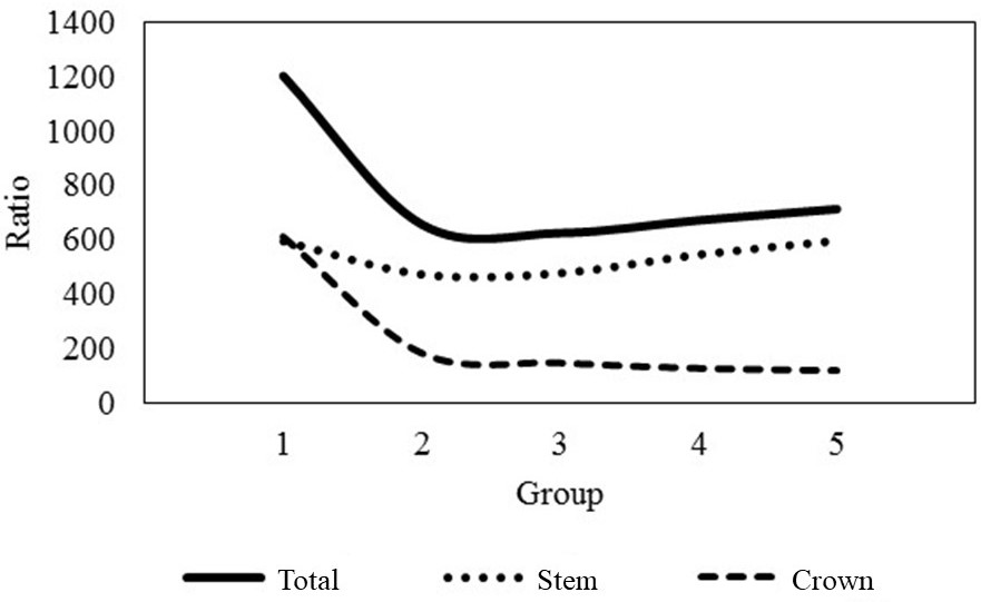
The equations (57) and (58) are, therefore, adjusted in (113) and (114), and presented in Figure 2.

Variation of the ratio between the biomass of the components and the total biomass with the stem volume in stands of black wattle in the state of Rio Grande do Sul, Brazil.
Explanations for the estimates obtained by means of this procedure are the same as those given for the first procedure presented in methods.
COMPARISON OF ESTIMATES USING RATIO AND REGRESSION ESTIMATES
Tables VII, VIII and IX shows the results of the statistics for comparison of the estimates trough ratio and WNSUR procedures.
Statistics obtained for comparison the estimates trough ratio and WNSUR procedures of stem biomass in stands of black wattle in the state of Rio Grande do Sul, Brazil.
Statistics obtained for comparison the estimates trough ratio and WNSUR procedures of crown biomass in stands of black wattle in the state of Rio Grande do Sul, Brazil.
Statistics obtained for comparison the estimates trough ratio and WNSUR procedures of crown biomass in stands of black wattle in the state of Rio Grande do Sul, Brazil.
DISCUSSION
Because most biomass studies are based on fitted volumetric models, i.e., using empirical data of biomass such as the predictor variables diameter at breast height (d) and the height of the tree (h), alone or combined, they often face heteroscedasticity of errors. Then, after the model is linearized, if appropriate, and the ordinary least squares is applied to estimate the parameters, this estimator ceases to be BLUE. This will affect the conclusions drawn on the significance tests of the equations used and the construction of confidence intervals for the coefficients, as well as the mean estimates and their prediction.
This heteroscedasticity of errors can be explained by its modeling, which follows a normal distribution with increasing variance in relation to Xi and is expressed by an exponential behavior of Xi, allowing the establishment of weights. In this way, the regression model can be adjusted by “generalized least squares, resulting in a BLUE estimator and, consequently, will validate the significance tests of the equation proposed and the construction of confidence intervals (Parresol 1999).
The two variables form factor F and wood density are associated with the coefficients of the regression models, however not setting up a balanced participation in the coefficients of each model when adjusted for the components, which leads to the loss of additivity. To solve this problem, several researchers have developed, since the 1970s, complex methodologies to force the additivity of components, known in the literature as SUR and NSUR (Kozak 1970, Chiyenda and Kozak 1984, Cunia and Briggs 1984, 1985, Reed and Green 1985, Parresol 1999, 2001PARRESOL BR. 2001. Additivity of nonlinear biomass equations. Can J For Res 31: 865-878.).
The model presented in this paper uses ratio estimates, in which the total biomass and the biomass of the components are function of the stem volume multiplied by the respective Scalar Coefficients Proxy of Density - SCPD. In this case, the assumption that the metric unit of the independent variables will assume the same metric unit of the dependent variable was assured and allowed to maintain the desired property in the biomass modeling: the additivity.
Considering the whole experience with biomass estimation presented in this work, especially those developed in Europe, it became apparent that the biomass estimators and carbon sequestration by trees were obtained with segmented models, i.e., each parameter of the model is estimated separately, avoiding problems with complex methodologies peculiar of linear regression models (Zianis and Mencuccini 2004, Chave et al. 2005, Saint-Andre et al. 2005, Vallet et al. 2006, António et al. 2007, Wutzler et al. 2008, Pretzsch 2009, Genet et al. 2011, MacFarlane 2015). For the same reason, the conceptual modeling proposed and performed in this work was obtained with a rational model, because it does not require extra methodological devices for additivity, as it was evidenced by the proof of Theorem 1 and its corollary. Even though the European experience has sought creative solutions to get a consistent estimator for the form factor (F) (Vallet et al. 2006, Genet et al. 2011), including the new variable called hardiness (hnd) to correct the effect of density in the form of trees, our experience has shown another way to deal with this estimator. We use the knowledge of the school of Freiburg, i. Br., Germany, which applies the concept of volume equivalence, in which, using the quadratic mean diameter () of stems, the volume taken at this reference shall be a cylinder equivalent to the stem volume referenced at the DBH (Prodan 1965, Ko 1968). Under these circumstances, the tree form factor shall be always equal to one and, therefore, enabling a solution for the relationship between () and (DBH), for which the accuracy of the mean estimate can be less than 4%. Such a solution is easy to implement in Brazilian companies, since they all have to collect sample data for adjusting volumetric equations and the data base has been gradually standardized with the Hohenadl’s methodology (Hohenadl 1924), as presented in this work.
Therefore, the results obtained by ratio estimates and WNSUR were similar, evaluated by the statistics ME, MAE MSE and RSME were also similar between the four different procedures and thus it is confirmed the second part of the proposed hypothesis.
The variable basic densities () were equated to be included in the proposed biomass models, considering the advantages of convenient properties of ratio estimates and because they are exactly the estimators per component. However, given the difficulty of obtaining experimentally the volumes of the components of each tree, we proposed to solve the problem relativizing them as a function of the stem volume. This transformation has converted the volumes of the components of each tree into Scalar Coefficients Proxy of Density - SCPD and, as it has been demonstrated in Theorem 1 and in its corollary, the additivity was maintained. Then, all the biomass estimators can be evaluated by taking only the stem volume and the respective ratio estimates already obtained experimentally.
Vallet et al. (2006) proposed the inclusion of a corrective term, adjusted as a function of age, to obtain a generic model for estimating biomass. To do so, they considered separately the estimates for the components and for total biomass. In the same way, a generic solution for the correction of the components and total biomass estimators for different ages was proposed in this research, taking advantage of a hyperbolic function fitted to the proportions of the SCPD as a function of the Scalar Proxy of Density of the stem to facilitate the obtaining of the other estimators that, despite changing their values, continue to maintain additivity with advancing of stand ages. This occurs because the biomass of components maintains a proportional behavior as age increases.
As we can see in the proposal presented in this work, the variable height was maintained to calculate the stem volume (Vs), considering its significant additional contribution in obtaining the stem and total volumes. However, it is evident the worldwide difficulty of measuring it in all trees. Normally, it is worth fitting hypsometric functions to provide all height values for the biomass equations. Vallet et al. (2006) emphasizes the importance of maintaining the height in the estimators for the additional contribution that it makes to obtaining the volumes. We consider appropriate to adjust a hypsometric model per plot, although in the present work it was done per forest area. If adjusting it per plot, it will be possible to indirectly mediate the effects of fertility or site variations, and stand density.
The model performed better for stem and total biomass than for crown biomass. Typically, the crown component is more difficult to model, since it is affected by several relational effects on its final configuration, mainly from the environment, and its inclusion in the biomass models is complex. MacFarlane (2015) dealt with this issue, although with restrictive aspects, as he assumed the existence of a central axis in the crown, a mean of crown diameter and an abstract form factor in order to obtain its volume. In the circumstances presented in this work, using the ratio estimate and a form factor equal to one, many of these problems were reduced to obtain a good estimate of the crown biomass.
The correlations observed between the variables included in the biomass model, using ratio estimates, indicated that the stem volume is an excellent independent variable for shaping it. The confidence intervals resulted in errors of less than 11% of the mean value in all cases. The adjustment of the mean quadratic diameter of the stem () as a function of d also proved entirely satisfactory, with a high correlation between the two variables and high accuracy, as already presented above. This shows that the adjustment of as a function of d by means of ratio estimate is appropriate. Balbinot et al. (2017)BALBINOT R, TRAUTENMÜLLER JW, CARON BO, BREUNIG FM, LAMBRECHT FR AND COSTA JÚNIOR S. 2017. Trunk biomass estimation by different methods in a Subtropical forest. Floresta 47(4): 553-560. have compared direct and indirect methods to estimate tree biomass of native species. The authors have concluded that direct method is the most effective way to quantify stem biomass, but indirect methods, that use estimated volume, did not differ statistically for the estimated and observed stem biomass.
The application of the adapted model, in which the total biomass or the biomass of the components is fitted as a function of the stem volume, estimated by diameter (d) and multiplied by the Scalar Coefficients Proxy of Density - SPDC, is also very appropriate, because additivity of the biomass components is maintained, a very desirable characteristic. Depending on the procedure, the model becomes indirectly dependent on d, a less costly and easier variable to be measured in the forest inventory.
All proposed and tested procedures resulted in acceptable explanations for the estimated coefficients and mean values, even with little variation between them. The estimation of coefficients to model the biomass of the components and total biomass as a function of the stem volume by ratio estimation method also proved very promising, because it is easy to solve, with only one division operation between two values and can be done quickly. Therefore, these estimators showed to be accurate and, especially, managed to preserve the natural biomass additivity, proving the hypothesis established in this study.
Ratio estimation may contribute beyond the biomass modeling, since it is possible to reduce the operational costs when applying it to forest inventory. It is known that the coefficients obtained by means of ratio estimates are dependent only on the means of the two variables involved, then the inventory should prioritize the evaluation of individuals from classes close to the means of the selected variables, thereby greatly reducing the sampling and, consequently, the costs.
The ratio estimates generate additivity for the tree components, in the same way they do for the tree data, whereas if they are modeled via linear or non-linear regressions, it is necessary to force it through SUR or NSUR methodologies to achieve additivity. In the proposed segmented estimators, the metric unit of the ratios are the same as those of the resulting coefficient, which was called Scalar Coefficient Proxy of Density, i.e., the metric unit of the ratios is kg.m-3 and, when multiplied by the value of the variable X will result in biomass in kg, which does not happen in almost all the volumetric models adapted to obtain biomass estimates. This confirms the first part of the proposed hypothesis.
The restriction on metrics of the dependent or independent variables in linear and non-linear regression models for biomass evaluation was applied because this is one of the significant reasons for not achieving additivity, i.e., it is modeling for indirect obtaining of biomass. In the case of our proposal, by the application of the ratio estimates, this condition is satisfied and, therefore, generates the natural additivity. This concept is not, of course, the real value of the basic density in the case of crown biomass, bark, or possibly only of the branches, because the cylindrical volume obtained experimentally is only for the stem. The variables arising in these cases, which were called Scalar Coefficient Proxy of Density, have characteristics of the metric unit of the basic density variable (kg.m-3). For the reasons given above, these variables were also obtained as a function of the cylindrical stem volume, owing to the high correlation that the tree biomass components have with it, as it is commonly used in allometric procedures in linear regression modeling. This reinforces the confirmation of the first part of the proposed hypothesis.
The approximate nature of the estimators, due to the actual values of density, has enabled us to ensure them consistency and absence of bias. This is acceptable in view of the difficulty in achieving the total volume of the tree with inclusion of branches, leaves or bark of the branches for precisely obtaining the density value of these components.
Additionally, even though assuming a linear or non-linear relationship of biomass with the variables diameter taken at 1.30 m (d) and tree height, it is implicitly accepting that this relationship is also being carried out based on an incomplete stem volume, as in the case of the Schumacher-Hall’s model or the Spurr’s model, being the only conceptual difference the presence of intercession in these models, which implies a solution only via linear or nonlinear regression.
The proposed method is simple and, as evidenced by the results obtained experimentally, are consistent and accurate. We emphasize that in all forest stands of Brazilian companies, because of the extraordinary genetic improvement achieved by them, tree volumes are used in the same way for adjusting volumetric equations and to obtain biomass estimates, as well as for the additional adjustment of a function to estimate the mean square diameter per tree, which can be easily done experimentally, therefore is quite appropriated for the purposes used in this work.
The generalization of the use of fitted functions for other components will be the result of a mere complement of statistical procedures for assessing the adequacy of the adjustments per forest area or, more generally, for an annual unit of planting (Figure 2).
Studies on the application of the proposed model should be expanded. It is also suggested the application of this modeling per diameter class.
CONCLUSIONS
The proposed model, using ratio estimates, is appropriate and promising for modeling of tree biomass.
The adjustment of the mean quadratic diameter of the stem () as a function of d also proved entirely satisfactory, with a high correlation between the two variables and high accuracy. This shows that the adjustment of as a function of d by means of ratio estimate is appropriate and is a key point for obtaining volumetric equivalence of tree components.
In the application of the adapted model, the total biomass, or biomass of components, are obtained as a function of the stem volume, which is estimated as a function of d and multiplied by the Scalar Coefficients Proxy of Density – SCPD. These integrated procedures are quite appropriate.
The use of a form factor equal to one for all the biomass components was a quite significant improvement in modeling biomass components. This approach means to transform their estimated volumes to equivalent real volumes avoiding, consequently, to have the adverse variation of this variable when it is present in the model as a random variable.
The natural additivity of the tree biomass components was fully achieved, when modeling them by means of ratio estimation.
Equations developed from the proportional behavior of the biomass components at different ages did not require the use of linear regression models and were obtained from calibration with the experimental data. The estimators resulting from these equations proved to be appropriate to make a generic model for correction of ratios coefficients at different ages.
The results obtained by ratio estimates and WNSUR were quite similar, evaluated by the statistics ME, MAE MSE and RSME, which were also similar between the four proposed procedures.
ACKNOWLEGMENTS
The authors thank to Conselho Nacional de Desenvolvimento Científico e Tecnológico (CNPq) for the Doctorate fellowship granted to the author Alexandre Behling, the company TANAC S.A./ TANAGRO S.A. for the research funding, the Centro de Excelência em Pesquisa em Fixação de Carbono em Biomassa (BIOFIX) of the Federal University of Paraná for allowing the use of its laboratory facilities, and Dr. José Valter Cotegipe Pélico for the special considerations on variable metrics in the quality of biological modeling, which encouraged the authors to propose the solution via ratio estimates.
REFERENCES
- ANTÓNIO N, TOMÉ M, TOMÉ J, SOARES P AND FONTES L. 2007. Effect of tree, stand, and site variables on the allometry of Eucalyptus globulus tree biomass. Can J For Res 37: 895-906.
- BALBINOT R, TRAUTENMÜLLER JW, CARON BO, BREUNIG FM, LAMBRECHT FR AND COSTA JÚNIOR S. 2017. Trunk biomass estimation by different methods in a Subtropical forest. Floresta 47(4): 553-560.
- BEHLING A, PÉLLICO NETTO S, SANQUETTA CR, CORTE APD, AFFLECK DLR, RODRIGUES AL AND BEHLING M. 2018. Critical analyses when modeling tree biomass to ensure additivity of its components. An Acad Bras Cienc 90: 1759-1774.
- BROWN JH, GILLOOLY JF, ALLEN AP, SAVAGE VM AND WEST G. 2004. Toward a metabolic theory of ecology. Ecology 85(7): 1771-1789.
- BROWN S. 1997. Estimating biomass and biomass change of tropical forests: a primer. FAO Forestry Paper 134.
- CANNELL MGR. 1984. Woody biomass of forest stands. For Ecol Manage 8: 299-312.
- CHAN N, TAKEDA S, SUZUKI R AND YAMAMOTO S. 2013. Establishment of allometric models and estimation of biomass recovery of swidden cultivation fallows in mixed deciduous forests of the Bago Mountains, Myanmar. For Ecol Manage 304: 427-436.
- CHAVE J ET AL. 2005. Tree allometry and improved estimation of carbon stocks and balance in tropical forests. Oecologia 145: 87-99.
- CHAVE J, CONDIT R, AGUILAR S, HERNANDEZ A, LAO S AND PEREZ R. 2004. Error propagation and scaling for tropical forest biomass estimates. Philos Trans R Soc B 359: 409-420.
- CHAVE J, COOMES D, JANSEN S, LEWIS SL, SWENSON NG AND ZANNE AE. 2009. Towards a worldwide wood economics spectrum. Ecol Lett 12: 351-366.
- CHAVE J ET AL. 2014. Improved allometric models to estimate the aboveground biomass of tropical trees. Glob Chang Biol 20: 3177-3190.
- CHIYENDA SS AND KOZAK A. 1984. Additivity of component biomass regression equations when the underlying model is linear. Can J For Res 14: 441-446.
- COCHRAN WG. 1963. Sampling Techniques. New York: J Wiley & Sons, 448 p.
- CUNIA T AND BRIGGS RD. 1984. Forcing additivity of biomass tables-add empirical results. Can J For Res 14: 376-384.
- CUNIA T AND BRIGGS RD. 1985. Forcing additivity of biomass tables: use of the generalized least squares method. Can J For Res 15: 23-28.
- DUCEY MJ. 2012. Evergreenness and wood density predict height–diameter scaling in trees of the northeastern United States. For Ecol Manage 279: 21-26.
- ENQUIST BJ. 2002. Universal scaling in tree and vascular plant allometry: toward a general quantitative theory linking plant form and function from cells to ecosystems. Tree Physiol 22: 1045-1064.
- ENQUIST BJ AND NIKLAS KJ. 2001. Invariant scaling relations across tree-dominated communities. Nature 410: 655-660.
- ENQUIST BJ, WEST GB, CHARNOV EL AND BROWN JH. 1999. Allometric scaling of production and life-history variation in vascular plants. Nature 401: 907-911.
- ENQUIST BJ, WEST JH AND WEST GB. 1998. Allometric scaling of plant energetics and population density. Nature 395: 163-165.
- GENET A ET AL.. 2011. Ontogeny partly explains the apparent heterogeneity of published biomass equations for Fagus sylvatica in central Europe. For Ecol Manage 261: 1188-1202.
- GOODMAN RC, PHILLIPS OL AND BAKER TR. 2014. The importance of crown dimensions to improve tropical tree biomass estimates. Ecol Appl 24(4): 680-698.
- GRAY HR. 1966. Principles of forest tree and crop volume growth: a mensuration monograph. National Development, Forestry and Timber Bureau, Canberra, 54 p.
- HOHENADL W. 1924. Der aufbau der baumschafte. Forstwiss Cbl 44: 17-18.
- HUXLEY JS. 1932. Problems of relative growth. London: Methuen & Co., Ltd., 276 p.
- JENKINS JC, CHOJNACKY DC, HEATH LS AND BIRDSEY RA. 2003. National-scale biomass estimators for United States tree species. Forest Sci 49: 12-35.
- KETTERINGS QM, COE R, VAN NOORDWIJK M, AMBAGAU Y AND PALM CA. 2001. Reducing uncertainty in the use of allometric biomass equations for predicting aboveground tree biomass in mixed secondary forests. For Ecol Manage 146: 199-209.
- KO YZ. 1968. Beziehungen zwischen formquotienten und formzadl. Doctoral thesis, Albert Ludwigs University.
- KOZAK A. 1970. Methods of ensuring additivity of biomass components by regression analysis. For Chron 46(5): 402-404.
- MACFARLANE DW. 2015. A generalized tree component biomass model derived from principles of variable Allometry. For Ecol Manage 354: 43-55.
- MOCHIUTTI S. 2007. Produtividade e sustentabilidade de plantações de acácia-negra (Acacia mearnsii De Wild.) no Rio Grande do Sul. Tese de doutorado, Universidade Federal do Paraná.
- NIKLAS KJ. 1994. Plant allometry: the scaling of form and process. Chicago: University of Chicago Press, 412 p.
- NIKLAS KJ. 1995. Size-dependent allometry of tree height, diameter and trunk-taper. Ann Bot 75: 217-227.
- NIKLAS KJ. 2004. Plant allometry: is there a grand unifying theory? Biol Rev 79: 871-889.
- PARRESOL BR. 1999. Assessing tree and stand biomass: a review with examples and critical comparisons. Forest Sci 45: 573-593.
- PARRESOL BR. 2001. Additivity of nonlinear biomass equations. Can J For Res 31: 865-878.
- PICARD N, SAINT-ANDRÉ L AND HENRY M. 2012. Manual for building tree volume and biomass allometric equations: from field measurement to prediction. Food and Agricultural Organization of the Unites Nations and Centre de Coopération Internationale en Recherche Agronomique pour le Développement, Rome and Montpellier, 215 p.
- PRETZSCH H. 2009. Forest Dynamics, Growth and Yield. Berlin: Springer, 664 p.
- PRODAN M. 1965. Holzmesslehre. Sauerlanger’s Verlag, Frankfurt am Main.
- REED D AND GREEN EJ. 1985. A method of forcing additivity of biomass tables when using nonlinear models. Can J For Res 15: 1184-1187.
- SAINT-ANDRE L, M’BOU AT, MABIALA A, MOUVONDY W, JOURDAN C, ROUPSARD O, DELEPORTE P, HAMEL O AND NOUVELLON Y. 2005. Age-related equations for above- and below-ground biomass of Eucalyptus hybrid in Congo. For Ecol Manage 205: 199-214.
- SANQUETTA CR, WOJCIECHOWSKI J, CORTE APD, BEHLING A, PÉLLICO NETTO S, RODRIGUES AL AND SANQUETTA MI. 2015. Comparison of data mining and allometric model in estimation of tree biomass. BMC Bioinformatics 16(247): 1-9.
- SAVAGE VM, DEEDS EJ AND FONTANA W. 2008. Sizing up allometric scaling theory. PLoS Comput Biol 4: 17.
- SCHUMACHER FX AND HALL FS. 1933. Logarithmic expression of timber-tree volume. J Agric Res 47(9): 719-734.
- SPURR SH. 1952. Forest inventory. New York: The Ronald Press Company, 476 p.
- SUKHATME PV, SUKHATME BV, SUKHATME S AND ASOK C. 1984. Sampling theory of surveys with application. Iowa: Iowa State College Press, 452 p.
- VALLET P, DHOTE JF, MOGUEDEC GL, RAVART M AND PIGNARD G. 2006. Development of total aboveground volume equations for seven important forest tree species in France. For Ecol Manage 229: 98-110.
- WEISKITTEL AR, MACFARLANE DW, RADTKE PJ, AFFLECK DLR, TEMESGEN H, WOODALL CW, WESTFALL JA AND COULSTON JW. 2015. A Call to Improve Methods for Estimating Tree Biomass for Regional and National Assessments. J For 113(4): 414-424.
- WEST GB AND BROWN JH. 2005. The origin of allometric scaling laws in biology from genomes to ecosystems: towards a quantitative unifying theory of biological structure and organization. J Exp Biol 208: 1575-1592.
- WEST GB, BROWN JH AND ENQUIST BJ. 1997. A general model for the origin of allometry scaling laws in biology. Science 276: 122-126.
- WEST GB, BROWN JH AND ENQUIST BJ. 1999. The fourth dimension of life: fractal geometry and allometric scaling of organisms. Science 284: 167-169.
- WEST GB, BROWN JH AND ENQUIST BJ. 2000. The origin of universal scaling laws in biology. In Scaling in Biology [Brown JH and West GW (Eds)], p. 87-112. New York: Oxford University Press.
- WUTZLER T, WIRTH C AND SCHUMACHER J. 2008. Generic biomass functions for Common beech (Fagus sylvatica) in Central Europe: predictions and components of uncertainty Can J For Res 38: 1661-1675.
- ZIANIS D AND MENCUCCINI M. 2004. On simplifying allometric analyses of biomass. For Ecol Manage 187: 311-332.
- ZIANIS D, MUUKKONEN P, MÄKIPÄÄ R AND MENCUCCINI M. 2005. Biomass and stem volume equations for tree species in Europe. Silva Fenn, 63 p.
Publication Dates
-
Publication in this collection
03 June 2019 -
Date of issue
2019
History
-
Received
14 Mar 2018 -
Accepted
18 June 2018