Activities of PMO optical space debris survey

Abstract

Space debris division of PMO is devoted to play an important role in the research of orbital mechanics and the development of space debris observation techniques in China. To support the work, this division builds and operates a large optical network across China. The observational network include two major subsets, large field survey telescopes and precise tracking telescopes. The main objective of the network is to maintain cataloged orbital debris and detect uncatalogued debris. CHES at YaoAn site is the most recent facility, for higher orbits survey. New operational software and data pipeline that aims at detecting unresolved objects has being developed. This paper presents the details of this facility and related activities.

Key words
telescope; survey; data reduction; space domain awareness

Introduction

The space debris division of Purple Mountain Observatory (PMO) is devoted in orbital mechanics research for decades. Due to the complexity of space environment, the long term observation is necessary for multiple work. In such a case, a dedicated optical network with modern techniques has been implemented from the beginning of this century.

As the fast growth of orbital objects’ quantity, more and more efforts have been spent in this area. CHES (CHanging Event Survey) is the most recent program for space debris survey, mainly aims at higher orbital objects cataloging and discovery. The first implementation has been put into operation at YaoAn site from 2018.

Facility

The main part of CHES-YaoAn is the successor of OTA (Optical Telescope Array) (Chen et al. 2013) with extreme large field coverage, but more like general astronomical survey system. It targets at higher orbital objects which move slower than lower orbital objects which are OTA’s main objective. The whole facility consists of a general survey subsystem which contains twelve smaller telescopes, a deep survey subsystem which contains two larger telescopes, and an all sky survey subsystem for observation supporting. Besides, there is also a central database for observation management and a cluster for data reduction. Figure 1 shows the connectivity of all these instruments.

Figure 1
CHES-YaoAn system overview: The system consists of 3 main parts, the large field survey array shown as TAS, the deeper field survey unit shown as TET, and an all sky camera shown as MASS. All the units are connected for unified management. The data center will converge all the observation resource and data product via database.

General Survey

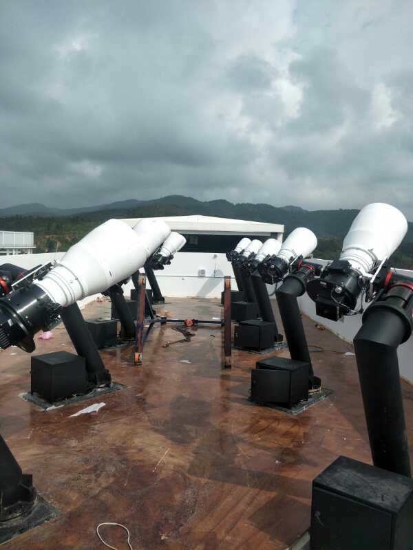
General survey subsystem contains 12 individual telescope units. The telescope tube of each unit is a customized APO (APOchromatic) refractor with 280 mm effective aperture and 300 mm focal length. Fully corrected and illuminated field is 55 mm to adapt the specific CCD (Charge-Coupled Device) chip size. Figure 2 shows the open status of its rolling roof and the telescope units. The designed APO optimized wavelength range is from 500 nm to 800 nm, to match the QE (Quantum Efficiency) of chosen CCD. This range can cover nearly whole bandwidth of SDSS r’ and i’ filter.

Figure 2
CHES-YaoAn large field survey array: This photo shows the large field survey array which consists of twelve 280 mm refractor under a RoR (Roll Off Roof).

Imaging detector is FLI^® ProLine9000 cooled CCD camera with ON Semi KAF-09000 front illuminated full frame CCD sensor, which has 3056 \(\times\) 3056 12\(\mu m\) pixels, and brings a square plane of 51.9 mm in diagonal. With 8MHz digitization speed, it will be less than \(1.8s\) for full frame readout. On this telescope, the actual field of view is \(7^{\circ} \times 7^{\circ}\), and \(8.25^{\prime\prime}\) per pixel. It means there is nearly 600 \(deg^2\) coverage for one exposure using the whole array. Camera filters including SDSS g’ r’ i’ and a customized open filter with 500-800 nm transmission are installed in FLI CFW-9-5 five-positions filter wheel. Considering the precise time tagging, all cameras share a time-server to record the real start and duration of the exposure. The timing latch is triggered by camera’s exposure active indicator signal, whose accuracy is higher than 1 ns.

All the telescope components are loaded on an ASA^® DDM85 Premium German equatorial mount. With the help of direct drive motor, the up to \(10^{\circ}/s\) slew speed can shorten the slewing time significantly. Mount is controlled by ASA Autoslew for Windows and connected to the operational program via ASCOM, which is a common standard for astronomical devices’ connectivity.

Each unit’s components are connected to a fan-less industrial computer running Windows 10. The unit’s operational program is written in Python 3. It communicates with mount, camera and filter wheel via ASCOM, reads time from clock server via RS485 serial port, acquires plans from central database, controls the whole observation procedure and reports the status of system and observation back to logging database. The observation plans are stored in plan database, and all units acquire the next plan independently with a predefined strategy after finishing the current plan. This makes all observation plans can be adjusted dynamically for the purpose of fast check and response. There is a quasi-realtime image reduction pipeline on each computer running under Linux subsystem for Windows. This pipeline is used for the preliminary image reduction, such as general pre-reduction, source extraction and astrometry calibration. All the results will be written back to the original fits image file as extended HDU (Header Data Unit).

With this set of telescope array, we can schedule different kinds of survey observation for different purposes. In SDA (Space Domain Awareness) work, what we care about with this facility are HEOs (Highly Elliptical Orbit) and GEOs (GEOsynchronous orbit). So we design several observation strategies and corresponding pipeline for moving objects searching and track association.

Deep Survey

To pursuit the sky coverage, the general survey subsystem compromise on accuracy and depth. Considering this, two complementary telescopes are set. They are ASA AZ800 prime focus reflector, with 800 mm aperture and f/2.26 focal ratio. Figure 3 shows one of these telescopes. Sensors are Andor^® iKon-XL 231. The final FoV is \(2^{\circ} \times 2^{\circ}\) with \(4108 \times 4096\) \(1.75^{\prime\prime}\) pixels.

Figure 3
CHES-YaoAn 800 mm prime focus telescope for deep survey. The telescope is AZ800 from an Austrian manufacture ASA, and the camera is a large format CCD iKon-XL 231 from Andor.

These telescopes will be used mainly for smaller field survey, such as follow-ups for confirmation, new objects searching, faint objects tracking. The better image quality can make sure the accuracy and depth of the system.

Computation

To support the operation and data reduction, a small on site cluster is used. There are disk arrays with more than 200 TB for data buffering. Four 16-cores computation nodes with 128 GB ram each are used for data reduction. The cluster is based on Debian GNU/Linux, and uses workload manager Slurm for computing resources allocation.

Operational program

Each telescope unit is operated unattended by an individual operational program. But telescope network is not only a stacking of many telescopes, there should have some kind of mechanism to coordinate the observation across the network. Considering the CHES survey program is a comprehensive observation coordination, in telescope type, location, scientific focus and so on, the operational program should take consideration of both flexibility and versatility.

Considering the scalability of the network, and the dynamical adjusting capability, we gave up the traditional big center scheme. Instead, we let each unit makes its own decision, using a common negotiation protocol between the control center and each unit. The manage center just continuously update assignments in a pool, according to the inputs from different sources and the feedback from operational units. It won’t become too heavier when the network grows, and the status of each unit will not interfere the function of the center.

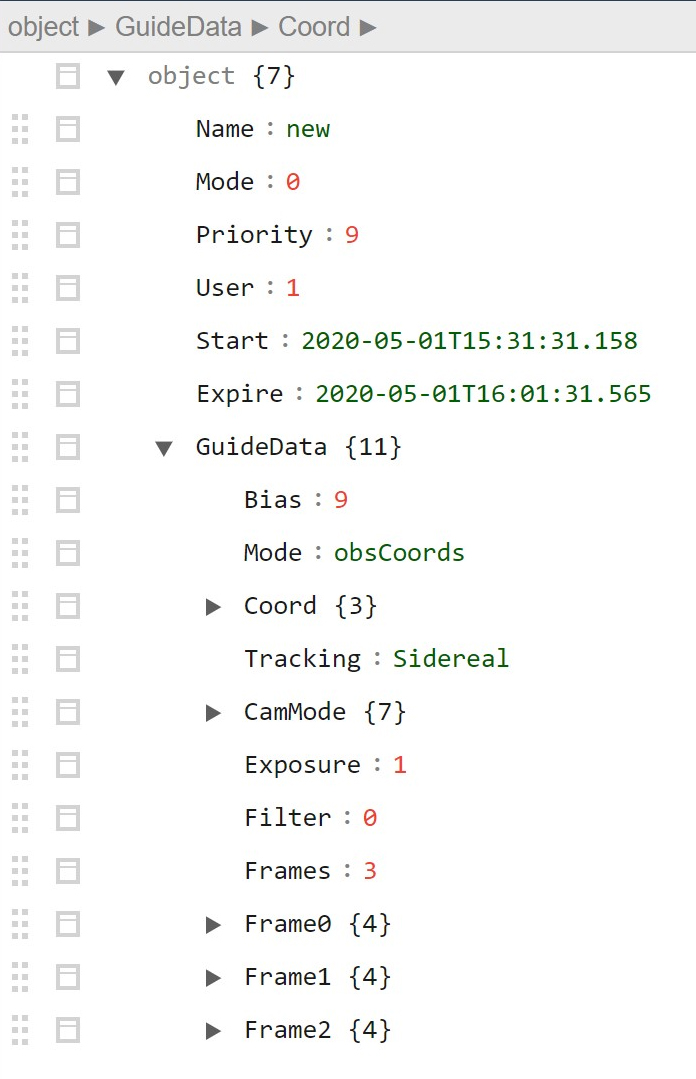
Different kind of observation request is described as one or several plans in this scheme. The description of each plan contains at least two parts, a common description for planner to query and a guiding description for operation guidance. The operational program on each unit will do the observation according to this information. Figure 4 shows a sample plan in Json format. All guiding description is in the key “GuideData,” other keys are common description.

Figure 4
A sample plan in Json format. The keys above GuideData are common description for planner to query, and the description in GuideData will tell the operational program how to do the observation, including at least target coordinates, tracking method, exposure setup, filter setup. This can be set uniform, or frame by frame if some keys are different, such as switches filter after each exposure.

Based on this scheme, we implement the first edition of the operational program. The program is divided into several modules as shown in Figure 5.

Figure 5
The Python program structure of observing system running on each unit.

• Daemon module runs as main thread that keeps the program alive and acts as the hub of other modules.

• Planner module queries plans from central database and makes the choice of most suitable plan currently. The decision system is parameterized for different use case optimization.

• Operator module is the abstract of different observation. It parses the information from guidance description and call the device to do the corresponding acts. The operations including normal frames at specified coordinates, RSO (Resident Space Object) tracking and special strategy survey. The operator can be extended easily cause it works as plugins to the main program.

• Device module is the actual code attached to the device hardware. This is the module that differs with different telescope units. Sometimes, the devices inside the unit have deeper connections and varies a lot, especially in professional telescope cases. So we don’t choose the normal implementation which combines standard parts together. The device module can use stardard ASCOM, Indi protocol or raw serial communication to connect the devices, in order to form basic actions, like startup, shutdown, slew, exposure, tracking and so on.

• HCI (Human Computer Interface) module is attached to the program as an optional thread, for manually operation and monitoring. The module use websockets and internal web server to provide human computer interface.

So, it should be easy to extend or replace some parts for different use. For example, to support different kind of telescope units, just make a new device model, but planner and operator modules can be reused. Currently, the code is written in Python 3, heavily dependent on Astropy and other python packages from astronomy community. This would help to make a larger network because it is easy to deploy to telescopes from professional to amateur.

Survey and methods

As the capability of general survey subsystem, it could survey the whole local sky within half an hour with 1 minute exposure. More specific, the site latitude is about 25 degree, so the sky coverage can reach 30 deg of southern hemisphere. We use 6 by 6 degrees size to make the field grid, considering the overlapping to reduce the effect of vignetting and degradation, the overlapping size is 0.5 deg on each side. The whole sky can be divided into 1160 fields of 36 sq.deg as shown in figure 6, but the visible sky at the same time as we defined the site local elevation above 25 deg (the air mass is about 2), is about 12000 sq.deg. It means about 332 to 340 fields at any time, as the field center is above 25 deg. For the all sky survey, these 12 telescopes could cover these fields together to achieve very fast visit.

Figure 6
The sky fields partition of all visible sky from YaoAn, based on the FoV of 280mm telescope. Each field is 6 x 6 degree, preserve 0.5 degree overlapping region on each edge, as the actual FoV of each telescope is 7 x 7 degree. The low declination and galactic latitude fields marked as red and black respectively.

Considering the importance of orbital resources, geosynchronous orbit (GEO) definitely is the most important one. Till now, more than 540 active objects stay in this region, play their key role in space missions. So this region needs much more attention to detect any abnormal activities as soon as possible, such as launches, break-ups, maneuvers. From 2018 to 2019, there were at least 4 major break-ups in higher earth orbits, 3 of their debris clouds go across the GEO protected region (Schildknecht et al. 2019). So, other than all sky survey, there is also extensive GEO survey (Zhao et al. 2016) figure 7. In our routine observation, we use general survey subsystem to maintain the catalog, and the deep survey subsystem to detect faint objects near the shadow cone (Africano et al. 2000).

Figure 7
The sky fields of GEO region from local sky of YaoAn, in azimuth coordinate. The 15 degrees north and south lines are the basic GEO region definition, and the green squares are the actual survey fields for one night, based on the dynamic pattern of GEO objects.

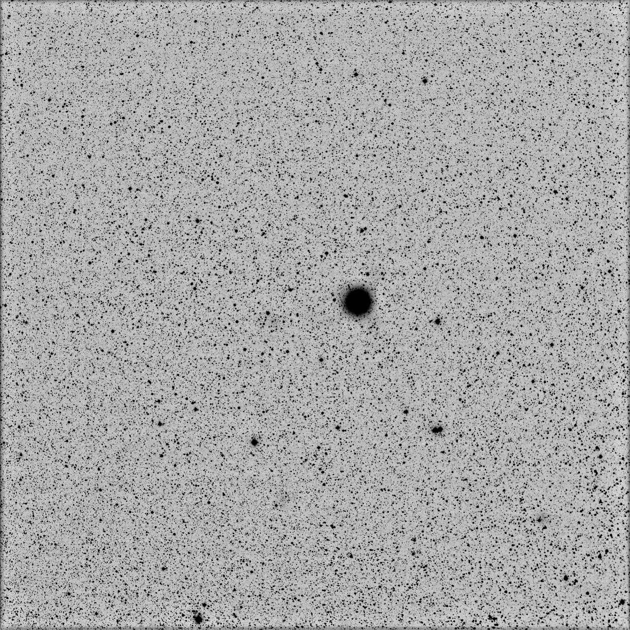
To take the consideration of GEO, MEO (Medium Earth Orbit) and HEO in the general survey, it is better to use sidereal tracking other than starring, to make more clear feature of separation between stars and RSOs. Each single exposure is 4 seconds. It is the longest exposure that the signal will accumulate in the same pixel for GEO objects, based on the actual FWHM and pixel size of the telescope optics. Figure 8 shows the typical image of one single exposure at very dense star field.

Figure 8
The typical image of one single exposure. Because of the dense star field which comes from the large field and pixel scale, it becomes very difficult to extract every single spot completely.

Each frame is reduced immediately with basic pre-reduction and astrometry calibration (Ping et al. 2018) pipeline. After finishing the whole group, the images will be sent to the cluster to be reduced by a moving object detection pipeline.

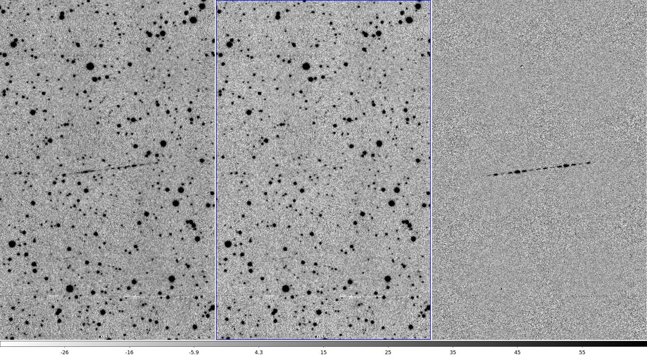
In the detection pipeline, first step is image differential. In spite of using sidereal tracking, there is still some deviation between frames during the several minutes tracking. So we use WCS information from astrometry calibration to reproject the images onto the same coordinate. We choose the bicubic interpolation method from reproject (Robitaille 2018) package to take the consideration of both performance and effect. Then produce local template with median stacking of these projected images. This would leave all the stars and remove all the moving objects, even their spots are overlapped. The differential image of each frame and this local template will only have moving objects left and some residuals of very bright stars. Final candidate catalogs of these images will be produced by sep (Barbary 2016) package. As shown in figure 9, the stars and moving objects are well separated.

Figure 9
The result of the image differential with local template. Left: mean stacking for comparing; middle: median stacking as local template; right: differential image with moving object trajectory left. The graph shows that the moving object has been separated from the stars completely, then we get a cleaned static sky and the changed part of the sky.

After the whole catalog collection is prepared, we will cross-match each catalog with the set of all the other catalogs in world coordinate system to remove all matched stars. This will filter the left over of bright stars from image differential process and faint stars around the detection limit as much as possible. Then put all the candidates together and map them onto a new image to do the trajectory detection with motion characteristic. Figure 10 shows a sample candidate map, the short lines are real objects, and the long horizontal line is caused by the defect of CCD camera.

Figure 10
Candidates map. From the changed part of every the frame, all sources have been extracted and mapped onto the same field to do the trajectory detection.

Figure 11
Detected candidate lines. Over plot all detected line segments onto the differential image of mean and median stacked images. This graph shows the line detection results at first step. This step is meant to detect all line features as much as possible.

To separate every object, the basic idea is to use the merged results of multiple loose constrains to converge better result than single tight constrain. The first constrain is based on line detection, as the object’s trajectory approximates straight line in pixel space. After comparing several line detection methods, we choose probabilistic Hough transform (Matas et al. 2000), and use the implementation from scikit-image python package (Van der Walt et al. 2014). Comparing to Hough transformation, this function detects line segments and runs faster.

Line segments only have correlation in space, and this is not reliable enough. So, the second constrain uses the correlation in coordinate-time space. The RA and Dec are linear over time within short time span. But in some cases, there will be more than one trajectory in a segment other than outliers, especially in GEO region because of the high density of objects there. So simply kick out the outliers with line fitting is not suitable. RANSAC (Raschka & Mirjalili 2019) algorithm can handle this, and we choose the implementation from scikit-learn (Pedregosa et al. 2011) python package. This kind of line fitting can tolerate a great number of outliers that definitely not belong to the target object. Iteration the left outliers can extract several trajectories from one data set. Shown as figure 12.

Figure 12
Trajectory separation using RANSAC line fitting. Using coordinates only in position space is not sufficient to separate very close trajectory, this usually happens in crowded orbits, such as GEO region. Adding time information can help. This graph shows the candidates in one line, X axis is relative time, and Y axis is right ascension of each point. From this collection, we can easily separate two targets using RANSAC line fitting.

Figure 13
Trajectories within whole field. The final detections are mapped onto the stacked image for reviewing. Each colored circles with number is an individual moving object.

Figure 14
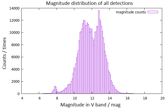
Magnitude distribution of all moving objects’ measurements. The detections in the statistics are all confirmed with a relatively strict criterion. X axis is V band magnitude and Y axis is the detections.

The Python implementation of this pipeline can reduce a set of 25 images in 5 to 10 minutes, in single thread on Dell T640 server with 2.3 GHz CPU. There are 4 nodes and each node can execute 16 jobs. So the consumption is acceptable to make sure the job will not accumulate in the waiting queue during the observation. This is key to the fast follow-ups.

Samples

Currently, CHES-YaoAn can do intensive GEO survey regularly. In this mode, the system can acquire measurements of more than 1000 objects. Take an example of observation at 2020-05-10, there are 1,028 objects as 26,983 trajectories which contain 409,602 measurements that are perfectly matched with the catalog. Among them, there are 457 GEOs, 334 HEOs, 81 MEOs and 156 other objects.

Besides, there are 243 possible hits with larger deviation, possibly due to the outdated orbits, or false alarms. The most interesting thing is that there are about 25 trajectories that cannot associate with any known object, but confirmed by manually image checking. These are objects that need to be focus on.

Future work

CHES-YaoAn can produce large amount of data, typically 2TB raw image per night. It is difficult for data management, transferring and storage. A compromise way is to buffer the raw images for a period as hot data, then make cold backup as compressed archive. Due to the major task of short exposure survey, we just keep the stacked images produced as local template, but two copies, mean and median stacking. So that, moving objects as well as separated stars can be retained as much as possible. The archive size of each day is about 40 GB, and can be moved to center storage by tape every month.

This provides opportunities of re-using the data for other scientific goals. In traditional way, we have used the network to do NEO (Near Earth Object) and GCN (Gamma-ray Coordination Network) follow-ups, like the newly discovered NEO 2020 DM4 (Minor Planet Center code aka MPC code) early stage follow-up. Furthermore, we can extract many valuable results other than SDA, from the data archive. 2020 FB7 (MPC code) is a NEO that fly by earth very close and fast, the magnitude drops from 11.2m to 20.3m in about 2 days. It was captured by CHES GEO survey when it went across the equator, and the trajectory did not match any of known earth orbital objects. After using the MPC guide information, it matches to the newly discovered NEO which found by ISON (International Scientific Optical Network). This shows that the large field coverage can be very useful for transient detection, but need more work on data pipeline. It is planned to do the extended data mining work in the form of cooperation with other groups.

Figure 15
Trajectory of 2020 FB7, a very fast NEO. We caught it using the large field survey and confirm it with MPC ephemeris. The image is mean stacked with multiple frames.

Summary

The research and development activity of CHES survey program is aimed at establishing technologies for detection and cataloging of higher orbital objects. This paper describes the first implementation at YaoAn site to pursue this goal. Technologies developed here will be used onto more telescopes, to enlarge the survey program, in China and global.

ACKNOWLEDGMENTS

This research was supported by the National Natural Science Foundation of China (Grant Nos. 11533010 and 11603082).

REFERENCES

• AFRICANO J, SCHILDKNECHT T, MATNEY M, KERVIN P, STANSBERY E & FLURY W. 2000. A geosynchronous orbit search strategy. Space Debris 2(4):357–369.
• BARBARY K. 2016. SEP: Source extractor as a library. J Open Sour Soft 1(6):58.
• CHEN Z ET AL. 2013. Space objects photometry using optical telescope array. Space Debris Research.
• MATAS J, GALAMBOS C & KITTLER J. 2000. Robust detection of lines using the progressive probabilistic hough transform. Comput Vis Image Underst 78(1):119–137.
• PEDREGOSA F ET AL. 2011. Scikit-learn: Machine learning in python. J Machine Learn Res 12:2825–2830.
• PING Y, ZHANG C & LU C. 2018. The Representation of OTA Images’ Astrometric Results with WCS-SIP Coefficientstwo. Chin Astron Astrophys 42(2):267–278.
• RASCHKA S & MIRJALILI V. 2019. Python Machine Learning: Machine Learning and Deep Learning with Python, Scikit-learn, and TensorFlow 2. Packt Publishing Ltd.
• ROBITAILLE T. 2018. Reproject: astronomical image reprojection in Python. Zenodo 10.
• SCHILDKNECHT T, VANANTI A, CORDELLI E & FLOHRER T. 2019. ESA optical surveys to characterize recent fragmentation events in GEO and HEO. Amos, p. 34.
• VAN DER WALT S, SCHÖNBERGER J, NUNEZ-IGLESIAS J, BOULOGNE F, WARNER J, YAGER N, GOUILLART E & YU T. 2014. Scikit-image: Image processing in Python. PeerJ 2:e453.
• ZHAO C-Y, ZHANG M-J, YU S-X, XIONG J-N, ZHANG W & ZHU T-L. 2016. Variation ranges of motion parameters for space debris in the geosynchronous ring. Astrophys Space Sci 361(6):196.

Publication Dates

• Publication in this collection
  23 Apr 2021
• Date of issue
  2021

History

• Received
  1 June 2020
• Accepted
  5 Sept 2020