Selecting “the best” nonstationary Generalized Extreme Value (GEV) distribution: on the influence of different numbers of GEV-models

ABSTRACT

The selection of an appropriate nonstationary Generalized Extreme Value (GEV) distribution is frequently based on methods, such as Akaike information criterion (AIC), second-order Akaike information criterion (AICc), Bayesian information criterion (BIC) and likelihood ratio test (LRT). Since these methods compare all GEV-models considered within a selection process, the hypothesis that the number of candidate GEV-models considered in such process affects its own outcomehas been proposed. Thus, this study evaluated the performance of these four selection criteria as function of sample sizes, GEV-shape parameters and different numbers candidate GEV-models. Synthetic series generated from Monte Carlo experiments and annual maximum daily rainfall amounts generated by the climate model MIROC5 (2006-2099; State of São Paulo-Brazil) were subjected to three distinct fitting processes, which considered different numbers of increasingly complex GEV-models. The AIC, AICc, BIC and LRT were used to select “the most appropriate” model for each series within each fitting process.BIC outperformed all other criteria when the synthetic series were generated from stationary GEV-models or from GEV-models allowing changes only in the location parameter (linear or quadratic). However, this latter method performed poorly when the variance of the series varied over time. In such cases, AIC and AICc should be preferred over BIC and LRT. The performance of all selection criteria varied with the different number of GEV-models considered in each fitting processes. In general, the higher the number of GEV-models considered within aselection process, the worse the performance of the selection criteria. In conclusion, the number of GEV-models to be used within a selection process should be set with parsimony.

Key words
Monte Carlo; GEV; MIROC5; downscaling

INTRODUCTION

Changes in frequency and intensity of extreme hydrometeorological events have been observed in virtually all regions of the world (Alexander et al. 2006; Fischer and Knutti 2015; Pereira et al. 2018). Therefore, it is now widely accepted that models assessing the probability of extreme weather events (e.g. the Generalized Extreme Value (GEV) distribution) should account for the presence of nonstationarities, such as those associated with interannual or interdecadal climate variabilities or with the global warming (Parker et al. 2007; Fischer and Knutti 2015). On such context, methods estimating the GEV-parameters under nonstationary conditions have been developed and used in several studies. Based on the principle of maximum likelihood, Coles (2001), Kharin and Zwiers (2005), Wang et al. (2004), Felici et al. (2007) and Blain (2011) estimated the GEV-parameters as linear, log-linear or quadratic functions of a given covariate (e.g. time). El Adlouni et al. (2007) and Hundecha et al. (2008) also modelled GEV-parameters as polynomial functions of time. However, these latter studies used a Bayesian approach known as Generalized Maximum likelihood (GML) (Martins and Stedinger 2000; El Adlouni et al. 2007), which intends to eliminate invalid values of the shape parameter of the GEV distribution. Cannon (2010) proposed using a conditional density network (CDN) to estimate the GEV-parameters. By using neural networks, nonstationary GEV models (CDN-GEV) become capable of representing a wide range of linear and nonlinear relationships among covariates and the GEV-parameters (Cannon 2010).

The natural consequence of the possibility of modelling several combinations of GEV-parameters as a function of covariates (Coles 2001) is that several GEV-models with varying complexity may be proposed to assess the probability of extreme events. Therefore, the selection of “the most appropriate” model becomes a key step in the use of nonstationary GEV-models (Coles 2001; El Adlouni et al. 2007; Blain 2011; Kharin et al. 2018). This selection process is often based on the principle of parsimony, which states that the most parsimonious GEV function – capable of explaining as much of the variance in the data as possible – should be selected (Coles 2001; El Adlouni et al. 2007; Cannon 2010). Thus, increasingly complex GEV-models are proposed and the one that best balances the trade-off between improving the description of the generating process and increasing the number of model parameters, which increases uncertainties in quantile estimation, is selected (El Adlouni et al. 2007). Several statistical techniques can be used to select from among different models. Among these, Akaike information criterion (AIC), second-order Akaike information criterion (AICc; also known as corrected AIC for small sample sizes), Bayesian information criterion (BIC) and likelihood ratio test (LRT) are widely used (Coles 2001; Cannon 2010; Strupczewski et al.2001 a, b; Sugahara et al. 2009; Villarini et al. 2009, 2010; Kharin et al. 2018). AIC, AICc and BIC are derived from the Information-Theoretic approach (Burnham and Anderson 2002) and they can be used to select from among any set of GEV-models. LRT is a hypothesis test that is carried out under a pre-specified significance level (usually 5%) (Coles 2001) and it can only be applied to sets of nested models (Cahill 2003; Kim et al. 2017).

Panagoulia et al. (2014) evaluated the performance of AICc and BIC. This latter study used 16 nonstationary GEV-models, sample sizes equal to 20, 50 and 100 and shape parameter equal to -0.1, 0.0 and 0.1. Panagoulia et al. (2014) indicated that BIC tends to select the correct model more often, probably because it presents a tendency to select more parsimonious models than AICc (a feature that had already been observed by other studies such as Kadane and Lazar (2004)). AICc presented the best performance only when sample sizes were set to their smallest value (Panagoulia et al. 2014). Kim et al. (2017) evaluated the performance of AIC, AICc, BIC and LRT for a larger range of sample sizes (from 30 to 160), shape parameters (from -0.2 to 0.2) and for four increasingly complex GEV models, in which the location and the scale parameters were allowed to linearly (log-linearly) vary over time. In spite of the difference between the Monte Carlo experiments performed by Panagoulia et al. (2014) and Kim et al. (2017), this latter study also indicated that AIC tends to select more complex GEV-models than the other criteria. Therefore, when the true model presented (linear) non-stationarities in both location and scale parameters, AIC outperformed all other selection criteria, including BIC (Kim et al. 2017). For other nonstationary cases evaluated in this latter study, AIC also outperformed all other selection criteria, including AICc, when the sample sizes were set to their smallest values. In such nonstationary cases, BIC presented the best performance as the sample sizes increased (Kim et al. 2017).

In spite of the methodological differences among AIC, AICc, BIC and LRT, they are all based on the comparison of all GEV-models used in the selection process. This suggests the hypothesis that the number of candidate GEV-models used in a particular selection process affects its own outcome. In simple terms, one may argue that if a different number of nested candidate GEV-models had been considered within a particular selection process, the result of such a process would have been different. For instance, suppose a common case in which the GEV distribution has been used to detect trends in a given long-term extreme rainfall or air temperature series (Blain 2011). In such case, three increasingly complex models were used to describe the relationships between a covariate (e.g. time) and the GEV-parameters. The first model assumed all GEV-parameters were constant over time (the stationary model); the second model estimated the location parameter as a linear function of time (the other two parameters remained constant; homoscedastic model) and the third model estimated, respectively, the location andthe scale parameters as linear and log-linear functions of time. Finally, suppose the stationary model has been selected from a process based on AIC criteria. The above-mentioned hypothesis leads to the following questions: this result, which may be regarded as an evidence suggesting the presence of no trend in this hydrometeorological series, could be different if more complex models had been used within the selection process? This result might be different if more complex models and different selection criteria (e.g. BIC or AICc) were used?

In order to provide information on this hypothesis, the goal of this study was to evaluate the performance of these four selection criteria (AIC, AICc, BIC and LRT) as function of different sample sizes (30 to 100), different GEV-shape parameters (-0.50 to 0.50) and different numbers of increasingly complex GEV-models used within three different selection process. Therefore, as further described in Methodology and Data Section, synthetic series were generated from five increasingly complex GEV nonstationary models for each combination of sample size and shape parameter. These nonstationary GEV-models are referred to as “true models”. Each synthetic series were subjected tothree different fitting processes. Within the first fitting process, each synthetic series was used to fit the parameter of three linear GEV-models. The first GEV-model assumed all GEV-parameters are constant; the second GEV-model estimated the location parameter as a linear function of time (the other two parameters remained constant) and the third GEV-model estimated, respectively, the location and the scale parameters as linear and log-linear functions of time. Among these three linear GEV-models, AIC, AICc, BIC and LRT were used to select “the most appropriate” model for each synthetic series. Within the second fitting process, the same synthetic series were used to fit the parameter of seven GEV-models. The first three GEV-models were the same as those used in the first process. The other four models allowed nonlinear changes in location and scale parameters. From among these seven models, AIC, AICc, BIC and LRT were again used to select “the most appropriate” model for each synthetic series. A third fitting process considered the first five models of the second fitting process. Among these five models, AIC, AICc, BIC and LRT were again used to select “the most appropriate” model for each synthetic series.

Finally, as a case of study, these three above-described fitting processes were applied to annual maximum values of daily rainfall amounts (2006 to 2099 under RCP 8.5) generated by a climate model participating in the 5^th Coupled Models Intercomparison Project Phase 5 (CMIP5; MIROC5) of NASA Earth Exchange Global Daily Downscaled Projections (NEX-GDDP) database. These datasets are to provide a set of global, high resolution, bias-corrected climate change projections that can be used to evaluate climate change impacts on processes that are sensitive to finer-scale climate gradients and the effects of local topography on climate conditions (Thrasher et al. 2012). As further described in Methodology and Data Section, the results of these different fitting processes were compared to each other.

METHODOLOGY AND DATA

Selection criteria

As previously described, AIC, AICc and BIC are calculated for all candidate models considered in a fitting process, and the model presenting the smallest value may be selected (Burnham and Anderson 2002). On the other hand, LRT can only be applied to pairs of nested GEV-models presenting different number of parameters (Kim et al. 2017). LRT is a hypothesis test and it null hypothesis assumes no difference between two nested models. Under such hypothesis, LRT is distributed according to a chi-square distribution with degrees-of-freedom equal to the difference between the number of each model parameters. LRT (Eq. 1) was carried out at 5% significance level. Therefore, values of LRT greater than the 95^th quantile of the chi-square distribution led to the conclusion that the M_j model is better than the M_i model.

$$\mathrm{LRT}=\left\{\log \left({\mathrm{ML}}_{\mathrm{j}}\right)-\log \left({\mathrm{ML}}_{\mathrm{i}}\right)\right\}\mathrm{for}{\mathrm{M}}_{\mathrm{i}}\mathrm{C}{\mathrm{M}}_{\mathrm{j}}$$ (1)

where log (ML) is the maximized log likelihood function.

AIC, AICc and BIC are calculated by Eqs. 2 to:

$$\mathrm{AIC}=-2\log \left(\mathrm{ML}\right)+2\mathrm{k}$$ (2)

where log (ML) is the maximized log likelihood function under the proposed model and k is the number of parameters in a given model. When the ratio between sample size (n) and number of model’s parameters (k) is less than 40, the use of AICc instead of AIC has been suggested (Burnham and Anderson 2002; Fabozzi et al. 2014).

$$\mathrm{AICc}=-2\log \left(\mathrm{ML}\right)+2\mathrm{k}+\frac{2\mathrm{k}(\mathrm{k}+1)}{\mathrm{n}-\mathrm{k}-1}$$ (3)

Bayesian information criterion (BIC) is also based on information theory and it is calculated by Eq. 4:

$$\mathrm{BIC}=-2\log \left(\mathrm{ML}\right)+\mathrm{klog}\left(\mathrm{n}\right)$$ (4)

As previously described, the GEV-model presenting the lowest BIC value may be regarded as the best candidate model.

Extreme value distribution (GEV)

Extremal Types Theorem, which within the statistic of extreme values is analogous to Central Limit Theorem, states that the maxima of independent and identically distributed data may be described by the Generalized Extreme Value (GEV) distribution (Coles 2001; Wilks 2011). GEV is a three-parameter function in which location (μ), scale (μ) and shape (ξ) parameters define, respectively, the position of the function in respect to the origin, spread of the distribution and its tail behaviour (Delgado el al. 2010). As others parametric distributions, GEV-parameters can be estimated from a data sample X comprising x_i data (i=1 to n; n is the sample size): Pr[x≤X]=GEV(x_i|μ,μ,ξ). In this latter form, the use of GEV is called classical or stationary approach (Coles 2001; El Adlouni et al. 2007; Cannon 2010), because it assumes the underlying process is stationary. However, as previously described, there has been several efforts adapting and improving the use of GEV when the assumption of stationarity may no longer be valid (Coles 2001; El Adlouni et al. 2007; Kharin et al. 2018). Therefore, as previously described, methods allowing for nonstationarities in GEV-parameters have been proposed by several previous studies (Coles 2001; El Adlouni et al. 2007; Cannon 2010). Among these methods, GEV-CDN (Cannon 2010) is capable of representing the widest range of relationships among GEV-parameters and covariates. This method estimates GEV-parameters by means of a conditional density network, which is a probabilistic extension of the multilayer perceptron neural network (Cannon 2010). GEV-CDN is also based on the generalized maximum likelihood method, so that GEV-shape parameter ranges from -0.5 to 0.5 according to a Beta distribution (Martins and Stedinger 2000; El Adlouni et al. 2007). CDN-GEV can replicate GEV models evaluated in other studies (Martins and Stedinger 2000; Coles 2001; El Adlouni et al. 2007). In addition, it can also model other forms of nonlinearity such as higher-order polynomial relationships (Cannon 2010). Therefore, CDN-GEV has been used in this study. Further information on GEV-CDN can be found in Cannon (2010). The cumulative and quantile function [F^-1 (1- p; μ,μ,ξ), 0 < p < 1] of the nonstationary GEV distribution can be described by Eqs. 5 and 6:

$$\mathrm{F}\left(\mathrm{x}\right)=\exp \left[-{\left\{1+{\mathrm{\xi }}_{\mathrm{t}}\frac{\mathrm{x}-{\mathrm{\mu }}_{\mathrm{t}}}{{\mathrm{\sigma }}_{\mathrm{t}}}\right\}}^{-1/{\mathrm{\xi }}_{\mathrm{t}}}\right]$$ (5)

$${\mathrm{F}}^{-1}\left(1-\mathrm{p};\mathrm{\mu },\mathrm{\sigma },\mathrm{\xi }\right)=\left\{\begin{array}{l}\mathrm{\mu }+\mathrm{\sigma }/\mathrm{\xi }\left\{{\left[-\mathrm{In}\left(1+\mathrm{p}\right)\right]}^{-\mathrm{\xi }}-1\right\},\mathrm{\xi }\ne 0\\ \mathrm{\mu }+\mathrm{\sigma }/\mathrm{\xi }\left\{\left[-\mathrm{In}\left(1+\mathrm{p}\right)\right]\right\},\mathrm{\xi }\ne 0\end{array}\right.$$ (6)

where variable p (in Eq. 6) is a probability value of range 0 to 1; In Eq. 5: μ(t), σ(t) and ξ(t) are location, scales and shape parameters, which can be fitted as polynomial functions such as:

$$\mathrm{\mu }\left(\mathrm{t}\right)={\mathrm{\beta }}_0+{\mathrm{\beta }}_1{\mathrm{t}}^1+...+{\mathrm{\beta }}_{\mathrm{j}}{\mathrm{t}}^{\mathrm{j}}$$ (7)

$$\sigma \left(\mathrm{t}\right)=\exp \left({\mathrm{\sigma }}_0+{\mathrm{\sigma }}_1{\mathrm{t}}^1+...+{\mathrm{\sigma }}_{\mathrm{j}}{\mathrm{t}}^{\mathrm{j}}\right)$$ (8)

$$\xi \left(\mathrm{t}\right)={\mathrm{\lambda }}_0+{\mathrm{\lambda }}_1{\mathrm{t}}^1+...+{\mathrm{\lambda }}_{\mathrm{j}}{\mathrm{t}}^{\mathrm{j}}$$ (9)

where j ranges from 1 to J, which is the order of the polynomial function, t is a covariate, β, α and λ are the coefficients of the polynomial function.

Monte Carlo simulations

Generating synthetic series from each true model

Equations 10 to 14 were used to randomly generate 5000 synthetic series for each combination of sample size and GEV-parameters. As in several previous studies, including Fowler et al. (2010), the shape parameter remained constant within each trial (λ_j=0) and it assumed five distinct values among the trials (λ₀=-0.5, =-0.25, =0.00, =0.25, =0.5). The sample sizes varied from 30 to 100 by steps of 10. Five true models, similar to those proposed by El Adlouni et al. (2007) and Cannon (2010), have been considered in this study:

$$\mathrm{GEV}(0,0,0):\mu \left(\mathrm{t}\right)=0+0\mathrm{t};\mathrm{\sigma }\left(\mathrm{t}\right)=e^{(0+0\mathrm{t})}\mathrm{and}\mathrm{\xi }\left(\mathrm{t}\right)=\mathrm{\lambda }0$$ (10)

$$\mathrm{GEV}(1,0,0):\mu \left(\mathrm{t}\right)=0+0.2\mathrm{t};\mathrm{\sigma }\left(\mathrm{t}\right)=e^{(0+0.2\mathrm{t})}\mathrm{and}\mathrm{\xi }\left(\mathrm{t}\right)=\mathrm{\lambda }0$$ (11)

$$\mathrm{GEV}(1,1,0):\mu \left(\mathrm{t}\right)=0+0.1\mathrm{t};\mathrm{\sigma }\left(\mathrm{t}\right)=e^{(0+0.2\mathrm{t})}\mathrm{and}\mathrm{\xi }\left(\mathrm{t}\right)=\mathrm{\lambda }0$$ (12)

$$\mathrm{GEV}(2,0,0):\mu \left(\mathrm{t}\right)=0+0,3\mathrm{t}+0.005\mathrm{t}2;\mathrm{\sigma }\left(\mathrm{t}\right)=e^{(0+0\mathrm{t})}\mathrm{and}\mathrm{\xi }\left(\mathrm{t}\right)=\mathrm{\lambda }0$$ (13)

$$\mathrm{GEV}(2,2,0):\mu \left(\mathrm{t}\right)=0+0.3\mathrm{t}+0.005\mathrm{t}2;\mathrm{\sigma }\left(\mathrm{t}\right)=e^{(0+0.0005{\mathrm{t}}^2)}\mathrm{and}\mathrm{\xi }\left(\mathrm{t}\right)=\mathrm{\lambda }0$$ (14)

Fitting processes

Within the first fitting process, each synthetic series generated from all five true models was used to fit the parameter of three nonstationary GEV models (Fig. 1). The first model (Fig. 1a) assumed all GEV-parameters are constant; the second model estimated the location parameter as a linear function of time (the other two parameters remained constant; Fig. 1b) and the third model estimated, respectively, the location and the scale parameters as linear and log-linear functions of time (Fig. 1c). The linear nature of models 2 and 3 has been accomplished by setting the hidden-layer activation function of the GEV-CDN architecture to the identity function (Cannon 2010). Among these three linear GEV-models, AIC, AICc, BIC and LRT were used to select “the most appropriate” model for each synthetic series generated from the five true models (Eqs. 10 to 14). Considering N_right as the number of times a particular selection criterion selected a model matching the true model, the performance (R_right) of AIC, AICc BIC and LRT was expressed as:

$$R_{right}=\frac{N_{right}}{5000}\times 100$$ (15)

Figure 1
A neural network architecture based on Cannon (2010). (a) Model 1 – all GEV-parameters are constant (stationary case); (b) Model 2 – the location parameter varies as a linear function of time (the other two parameters remained constant); (c) Model 3 – location and scale parameters vary as linear and log-linear functions of time; (d) Model 4 – allows nonlinear change only in the location parameter with 1 hidden layers; (e) Model 5 – allows nonlinear changes in both location and scale parameters with 1 hidden layers; (f) Model 6 – allows nonlinear change only in the location parameter with 2 hidden layers; (g) Model 7 – allows nonlinear changes in both location and scale parameters with 2 hidden layers.

As previously described, this study also considered other two fitting process (second and third fitting process) that took into account linear as well as nonlinear GEV-models. The first three models of the second fitting process were the same as those used in the first process (Fig. 1a-c). The fourth model (Fig.1d) allowed a nonlinear change only on the location parameter. Having only one hidden-layer node, this 6-parameter function is the simplest nonlinear GEV-CDN model. The fifth model (Fig.1e) also has a single hidden-layer node but it allows nonlinear changes in both location and scale parameters (it is a 7-parameter function). As model 4, the sixth model (Fig. 1f) also allowed nonlinear change only on the location parameter; however, it has two hidden-layer nodes. Finally, the seventh model (Fig. 1g) has two hidden-layer nodes, allowing nonlinear changes in both location and scale parameters. This latter model is able to approximate second-order polynomial function as well as other more complicated functions such as a Z-shaped continuous curve (Christiansen 2005; Cannon 2010). Models six and seven have, respectively, 9 and 11 parameters. The third fitting process considered the first five models of the second fitting process (Fig. 1 a-e). Because of the sake of brevity, the results of this latter fitting process are presented in the Supplementary File. Both second and third fitting processes were applied to all series generated from all true models. At this point, it becomes worth mentioning that the true models GEV(2,0,0) and GEV(2,2,0) are nonlinear quadratic GEV models. Therefore, fitting processes using only linear models, such as the first fitting process, cannot select the correct GEV-function for series that have been generated from these two (nonlinear) true models. This is the reason why the first fitting process could not be applied to the synthetic series generated from the above-mentioned nonlinear true models. Finally, AIC, AICc, BIC and LRT were used to select “the most appropriate” model for each trial and Eq. 15 (R_right) was used to evaluate the performance of each selection criteria within each fitting process.

Case study

The three fitting processes described in Fitting Processes Subsection were applied to annual maximum values of daily rainfall (block maxima approach) generated from a climate model – the MIROC model – participating in CMIP5 (Taylor et al. (2012). More specifically, the GEV models considered in these three fitting process have been fitted to four randomly chosen grid points (locations) of the State of São Paulo-Brazil: location 10 (48.375W and 25.125S; location 100 (48.625W and 23.625S; location 361 (48.125W and 21.625S); location 500 (47.125W and 20.125S) considering the greenhouse gas and aerosol forcing scenario RCP 8.5 for the period of 2006-2099 (van Vuuren et al. 2011). MIROC5 has already been used in studies addressing extreme weather conditions in the State of São Paulo (Fontolan et al. 2019). As in the simulation experiments, AIC, AICc and BIC were used to select the most appropriate model for each grid point and within each fitting process. Similar to the proposed method by Fowler and Kilsby (2003), the outcomes of each fitting processes have been compared to temporal change in both location and scale parameters of stationary GEV-models. The temporal change in both location and scale parameters of stationary GEV-models were evaluated from a 31-year moving window as suggested by Kharin and Zwiers (2005).

Finally, since the dispersion of any “real” rainfall series can change over time, three additional GEV-models [GEV(0,1,0), GEV(0,2,0) 1-hidden layer and GEV(0,2,0) 2-hidden layers] presenting changes in the scale parameter were considered in the fitting processes. More specifically, while the second fitting process also considered these three additional models, the third fitting process considered only the additional models GEV(0,1,0) and GEV(0,2,0) with 1-hidden layer. The first fitting process considered only the additional model GEV(0,1,0). As previously described, LRT can only be applied to pairs of nested GEV-models presenting different number of parameters (Kim et al. 2017). Therefore, this latter test could not be evaluated in this case of study, since the models GEV(1,0,0) and GEV(0,1,0) or GEV(2,0,0) and GEV(0,2,0) present the same number of parameters.

RESULTS AND DISCUSSION

GEV(0,0,0): The Stationary Model

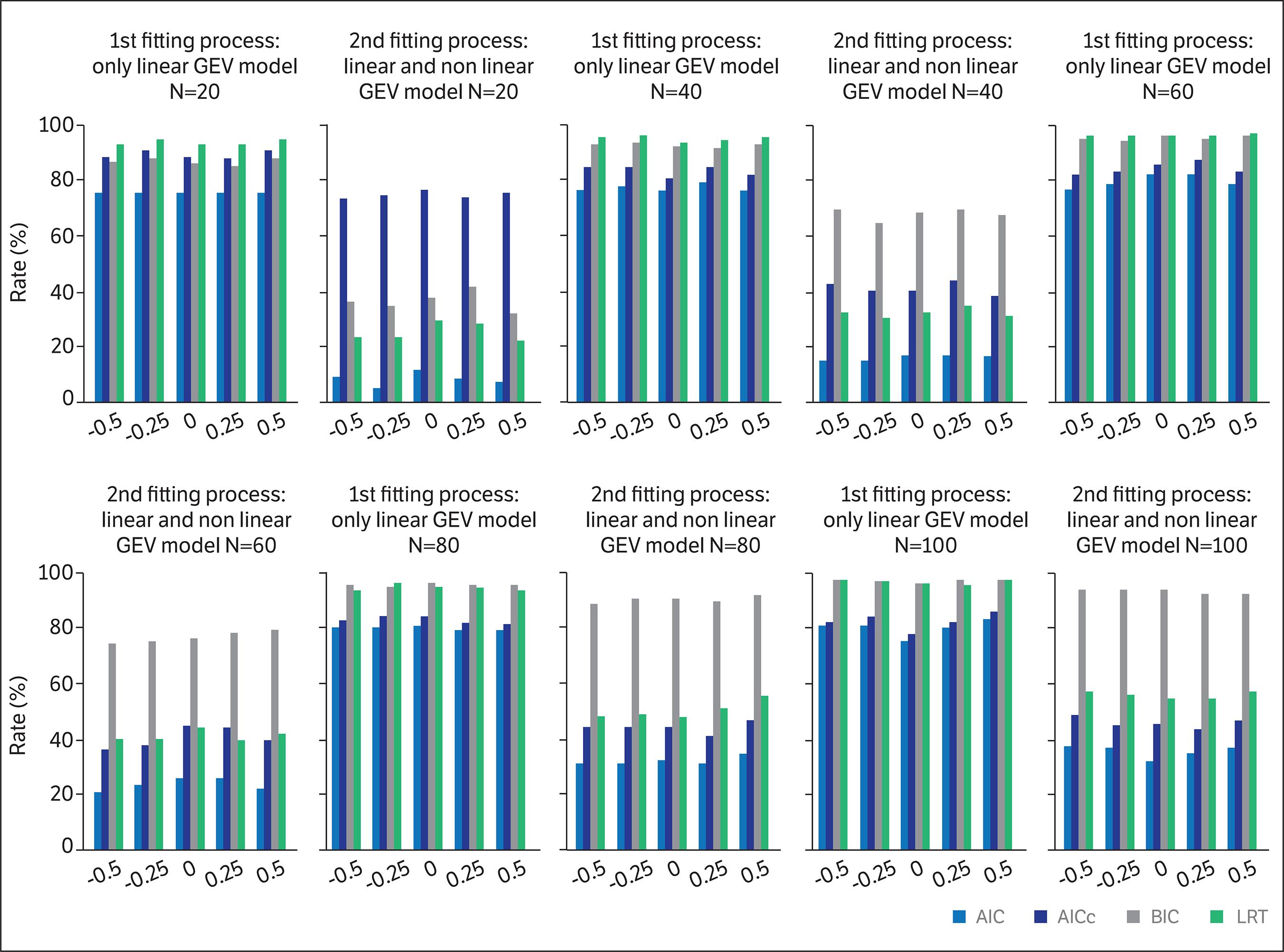
The performance of all selection criterium were clearly affected by the different number of candidate models considered in the three fitting processes (Fig. 2 and Supplementary File). In other words, the results of Fig. 2 are in line with the hypothesis of this study. As can be noted, there was a decrease in the performance of all selection criteria when a higher number of candidate models were considered in the fitting processes (Fig. 2). This latter statement is particularly true for those selection processes based on AIC, AICc and LRT, since the decrease in the performance of these criteria (fitting process 1 vs fitting process 2) can be observed for all combinations of sample sizes and shape parameter. The poor performance of both AIC and AICc in the second fitting process may be caused by their tendency to select more complex models than BIC (Panagoulia et al. 2014 and Kim et al. 2017). For instance, Model 7, which is the most complex model of this study, was the most selected by AIC within the second fitting process (not shown). AICc and LRT also selected model 7 at high rates within the second fitting process.

Figure 2
Rate (%) in which a particular selection criteria selected a GEV-model matching the true model used to generated the synthetic series. Akaike information criterion (AIC), second-order Akaike information criterion (AICc), Bayesian information criterion (BIC) and likelihood ratio test (LRT). The true model is the stationary GEV function.

Among all selection criteria evaluated in this set of Monte Carlo simulations (Fig. 2), BIC was the least affected by the different numbers of GEV-models considered in the two fitting processes. As observed by Panagoulia et al. (2014), BIC was outperformed by AICs only when the sample size was set to its smallest value (20). Nevertheless, even this latter selection criteria presented R_right rates approaching 90% in the second fitting process only for large sample sizes (equal to or larger than 80). This suggests that the use of complex nonstationary models, as those evaluated in the second fitting process, should be avoided when the sample size is smaller than 80. In general, all selection criteria improved their performance as GEV distribution approaches its second particular case known as Frechet or Fischer-Tippett type-II distribution (positive values of the shape parameter, considering the notation in Eqs. 5 and 6).This latter statement is particularly true for the second fitting process and it was also observed by Kim et al. (2017).

GEV(1,0,0): Only the location parameter linearly vary over time

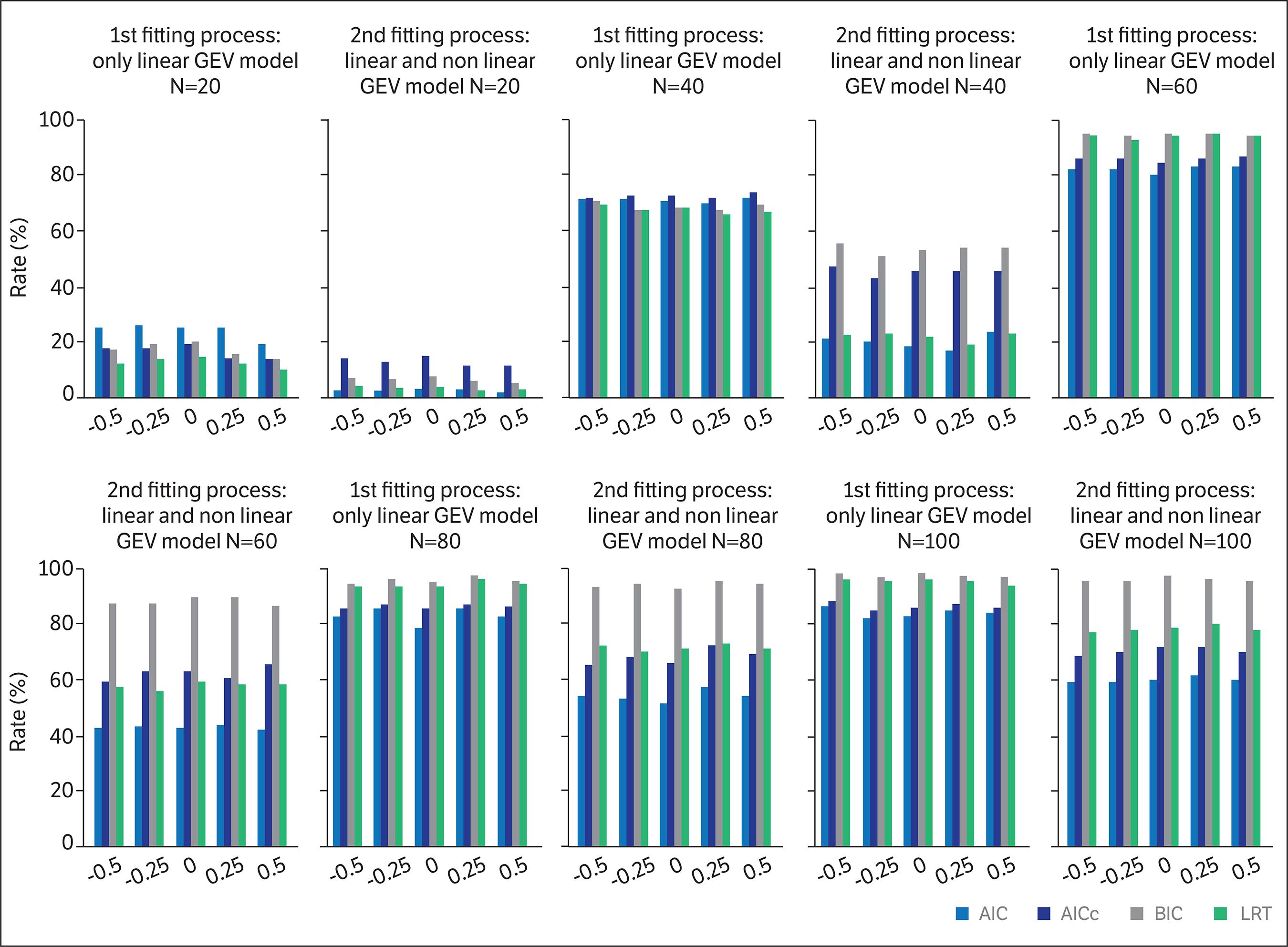
As observed in the stationary case, the performance of all selection criteria were clearly affected by the different number of GEV-candidate models considered in the three fitting processes. Again, the higher number of GEV models considered in the second and third fitting processes led to a decrease inthe performance of all selection criteria. As observed in (stationary case), AIC, AICc and LRT performed poorly when linear and nonlinear models were considered in the fitting process (Fig. 3). BIC was again the least affected by the different numbers of GEV-models considered in the three fitting processes. The R_right rates of this latter criteria in the three fitting processes became equivalents to each other. They also became higher than 90% for sample sizes equal to or larger than 80. Finally, the R_right rates presented by BIC in the two fitting processes (Fig.3) are in agreement with those found by Panagoulia et al. (2014) and in disagreement with those found byKim et al. (2017).

Figure 3
Rate (%) in which a particular selection criteria selected a GEV-model matching the true model used to generated the synthetic series. Akaike information criterion (AIC), second-order Akaike information criterion (AICc), Bayesian information criterion (BIC) and likelihood ratio test (LRT). The true model is a nonstationary GEV function that allows the location parameter to vary linearly over time.

GEV(1,1,0): location and scale parameters linearly vary over time

As observed in the two previous sections, the performance of all selection criteria was negatively affected by the higher number of candidate models considered in the second and third fitting process (Fig. 4 and Supplementary File). However, when the results of this section – obtained from a GEV(1,1,0) model – are compared with those of the previous section – obtained from a GEV(1,0,0) –the negative effect of the time-varying scale parameter onthe performance of all selection criteria becomes evident. In other words, the results depicted in Fig.4 allow us to indicate that increasing the variance of a series over time, decrease the ability of AIC, AICc, BIC and LRT to properly select a GEV-model.

Figure 4
Rate (%) in which a particular selection criteria selected a GEV-model matching the true model used to generated the synthetic series. Akaike information criterion (AIC), second-order Akaike information criterion (AICc), Bayesian information criterion (BIC) and likelihood ratio test (LRT). The true model is a nonstationary GEV function that allows both location and scale parameters to vary linearly over time.

Different from what was observed in the previous sections, AIC and AICc presented respectively the best and the second best performance within the first fitting process. This result is in line with those results found by Kim et al. (2017). Within the second fitting process, AICc outperformed all methods, including AIC, which presented the second best performance. The results of this section also suggest that when the variance of a series changes over time, both AIC or AICc tend to outperformance BIC and LRT.

GEV(2,0,0): location parameter quadratic vary over time

This and the next subsections are based on synthetic series generated from nonlinear quadratic GEV models. Therefore, as previously described, fitting processes using only linear models, such as the first fitting process, can never select the correct GEV-function (R_right rates will always be equal to zero for any selection criteria). This is the reason why Fig. 5 depicts the R_right rates for the second and third fitting processes. The nonlinear feature of the true model [GEV(2,0,0)] negatively affected the performance of all selection criteria (Fig. 5). For instance, no criteria except BIC presented R_right rates higher than 75%. This negative effect becomes evident when the R_right rates of Fig. 5 are compared with those of Fig. 3 which were obtained from the true model GEV(1,0,0). This statement holds true for any combination of shape parameter and sample size. BIC was the only criteria presenting R_right rate above 90%. However, these relatively high rates were achieved only when the sample size was set to its largest value (100).

In summary, the results of Fig. 5 are in line with those found in the previous sections – which were based on the homoscedastic GEV-models GEV(1,0,0) and GEV(2,0,0) – since they also indicated BIC as the best selection criterion. Nevertheless, the results depicted in Fig. 5 also indicate that even this latter criterion was capable of selecting the true quadratic model [GEV(2,0,0) at acceptable rates (>90%) only for considerable large sample sizes (≥100). The performance of this latter selection criterion within each fitting process approached each other as the sample size increased.

Figure 5
Rate (%) in which a particular selection criteria selected a GEV-model matching the true model used to generated the synthetic series. Akaike information criterion (AIC), second-order Akaike information criterion (AICc), Bayesian information criterion (BIC) and likelihood ratio test (LRT). The true model is a nonstationary GEV function that allows the location parameter to quadratic vary over time.

GEV(2,2,0): location and scale parameters quadratic vary over time.

The R_rates found in this section (Fig. 6) were similar to those found for GEV(1,1,0) model, which were based on a GEV-model presenting the location as well as the scale parameters as function of time. In other words,the results of this section also indicate that increasing the variance of a series over time, decrease the ability of all selection criteria in properly select the correct GEV model for this same series. Within the second fitting process, no criteria presented R_right rates higher than 90% for any combinations of shape parameter and sample size. BIC was the only criteria presentig R_right rate close to 85%. However, these latter R_right rates were achieved only when the sample size was set to its largest value (N=100; Fig. 6).As the results of Fig. 4, the results of the third fitting process (Fig. 6) also indicated that both AIC and AICc outperformed the BIC in identifying the correct model. Within the third fitting process, when the sample size was set to its largest value, AIC and AICc presented R_right rates higher than 95% (Fig. 6). In summary, the results of this section are in line with those found for GEV(1,1,0) model, suggesting that when there is a temporal change in the variance of the series, AIC or AICc are preferred over BIC. Nevertheless, it has to be mentioned that this latter recommendation hold true only for the third fitting process that considered nonlinear models with only one hidden layer. When a larger number of GEV-models were considered (second fitting process) no selection criteria presented R_right rates higher than 90%. This latter result, along with those of the previous sections, suggests that the number of GEV-models to be used within a selection process should be set with parsimony.

Figure 6
Rate (%) in which a particular selection criteria selected a GEV-model matching the true model used to generated the synthetic series. Akaike information criterion (AIC), second-order Akaike information criterion (AICc), Bayesian information criterion (BIC) and likelihood ratio test (LRT). The true model is a nonstationary GEV function that allows both location and scale parameters to quadratic vary over time.

Case study

Previous studies have applied nonstationary GEV-models to assess the probability of weather extremes under distinct climate scenarios (Kharin et al. 2013, Kharin et al. 2018). Some of these studies fitted increasingly complex GEV models to 20- or 30-year periods (e.g. 2011-2040; 2041-2070; 2071-2100) and used at least one of the four selection criteria (AIC, AICc, BIC or LRT) to evaluate how frequency and intensity of such events varied over time. However, the results of the sets of Monte Carlo simulations found in the previous sections indicate that these four selection criteria may present a poor performance when applied to small sample sizes. Therefore, they were applied to select GEV-models, which have been fitted from all available period (2006-2099).

The results of the sets of Monte Carlo experiments also indicated that the performances of all selection criteria are negatively affected when the variance of the series changes over time. These simulations also indicated that in such cases, both AIC and AICc should be preferred over both BIC and LRT. For location 10, the scale parameters of the stationary model – which specifies the dispersion ofthe series – significantly changed over time (Fig. 7). In the same pixel, the location parameter – which defines the central tendency of the distribution – also changed over time(Table 1). BIC failed to select nonstationary models describing these temporal changes in the variance of the series (2006-2099; Table 1). This statement holds true for the three fitting processes. Considering the first and the third fitting processes, both AIC and AICc have detected these changes in the central tendency and in the dispersion of the series by selecting GEV(1,1,0) models (Fig. 7). However, consideringthe second fitting process, both AIC and AICc failed to detect thechanges in the dispersion of the series, since these both methods selected a GEV(2,0,0) model. This latter result is in line with those found in the previous sections, since it also supports the general recommendation that the number of GEV-models to be used within a selection process should be set with parsimony.

Figure 7
The GEV-parameters (location or scale) estimated from 31-year moving window (solid line). The dashed line is the 95% confidence interval.

Table 1
Different GEV-models selected from three distinct criteria (AIC, AICc and BIC). GEV(0,0,0) is the stationary model; GEV(1,0,0) allows the location parameter to vary as a linear function of time (the other two parameters are constants); GEV(1,1,0) allows both location and scale parameter to vary as a linear function of time and; GEV(2,0,0) allows nonlinear change only in the location parameter. It has two hidden layers. Grid-Points 10, 100, 361 and 500 correspond, respectively to the following coordinates: 48.375W and 25.125S; 48.625W and 23.625S; 48.125W and 21.625S; 47.125W and 20.125S. State of São Paulo-Brazil.

Pixel	Selected Model
	1st fitting process
	AIC	AICc	BIC
10	GEV(1,1,0)	GEV(1,1,0)	GEV(0,0,0)
100	GEV(1,0,0)	GEV(1,0,0)	GEV(1,0,0)
361	GEV(1,0,0)	GEV(1,0,0)	GEV(0,0,0)
500	GEV(0,0,0)	GEV(0,0,0)	GEV(0,0,0)
Pixel	2nd fitting process
	AIC	AICc	BIC
10	GEV(2,0,0)	GEV(2,0,0)	GEV(0,0,0)
100	GEV(1,0,0)	GEV(1,0,0)	GEV(1,0,0)
361	GEV(1,0,0)	GEV(1,0,0)	GEV(0,0,0)
500	GEV(0,0,0)	GEV(0,0,0)	GEV(0,0,0)
Pixel	3rd fitting process
	AIC	AICc	BIC
10	GEV(1,1,0)	GEV(1,1,0)	GEV(0,0,0)
100	GEV(1,0,0)	GEV(1,0,0)	GEV(1,0,0)
361	GEV(1,0,0)	GEV(1,0,0)	GEV(0,0,0)
500	GEV(0,0,0)	GEV(0,0,0)	GEV(0,0,0)

For location 100, the three selection criteria have selected the same nonstationary model [GEV(1,0,0)]. In other words, AIC, AICc and BIC were able to detect the change in the location parameter observed in the same parameter of the stationary models (Fig. 7). This statement holds true. At such a location, the scale parameter has shown no remarkable change throughout the four sub-periods and over the 31-year moving window (Fig. 7).

At location 361, while BIC detected no change in GEV-parameters, both AIC and AICc selected GEV(1,0,0) in the three fitting processes (Table 1). In a first analysis, the steady increase presented by the location parameter after 2075 (see Fig. 7; pixel 361) may indicate that GEV(1,0,0) is indeed the best model for such a case. However, during the 2030s, this parameter presented values as high as those observed after 2075 (Fig. 7; pixel 361). Therefore, when compared with GEV(1,0,0), a stationary GEV model may be regarded as a better option. In location 500, GEV(0,0,0) model has been selected for all selection criteria within the three fitting process. This is in line with the parameters of the stationaries models fitted to the 31-year moving windows, which presented no significant change in their values (Fig. 7).

SUMMARY

Methods estimating the parameters of the Generalized Extreme Value (GEV) distribution as function of covariates have been proposed by several studies so that this distribution is now capable of representing a wide range of relationships among covariates and its parameters. On such background, the selection of “the most appropriate” GEV-model has become a key-step in the use of this nonstationary distribution. This selection is often based on statistical techniques, such as Akaike information criterion (AIC), second-order Akaike information criterion (AICc), Bayesian information criterion (BIC) and likelihood ratio test (LRT). Since all these methods are based on the comparison of all candidate GEV-models considered in the selection process, the hypothesis that the number of candidate GEV-models of a particular selection process affects its own outcome has been proposed. The goal of this study was to evaluate the performance of these four selection criteria as function of different sample size, different GEV-shape parameters (-0.50 to 0.50) and different numbers of increasingly complex GEV-models. Synthetic series generated from several Monte Carlo experiments were subjected to three distinct fitting processes, which considered different numbers of increasingly complex GEV-models. AIC, AICc, BIC and LRT were used to select “the most appropriate” model for each synthetic series within each fitting process. As a case of study, annual maximum daily rainfall amounts (2006 to 2099) generated by the climate model MIROC5 have also been subjected to the three above-mentioned fitting processes. The performance of all selection criteria was strongly affected by the different numbers of candidate models considered within each process. In general, the higher the number of models considered within a selection process, the worse the performance of the selection criteria. BIC outperformed all other criteria when the synthetic series were generated from stationary GEV-models or from GEV-models allowing changes only in the location parameter (linear or nonlinear). However, this latter method performed poorly when the variance of the synthetic series varied over time. In such cases, AIC and AICc should be preferred over BIC and LRT. The use of highly flexibly GEV-models based on a conditional density network with two hidden layers decreased the performance of all selection criteria in respect to that observed when only nonlinear GEV-models with one hidden layer have been considered. This latter statement holds true for the Monte Carlo experiments as well as for the case of study. In summary, since the results found in this study support our hypothesis, we recommend that the number of GEV-models to be used within a selection process should be set with parsimony.

ACKNOWLEDGEMENTS

This study is partly from PhD dissertation in development at the Agronomic Institute of Campinas (IAC). The authors thank the Climate Analytics Group and NASA Ames Research Center for providing NEX-GDDP database (distributed by the NASA Center for Climate Simulation; NCCS). Theauthors wish to acknowledge the Laboratory of Atmospheric Extremes Events (EAE) - Federal Technological University of Paraná (Londrina, Brazil) for the technological support.

REFERENCES

• Alexander, L. V., Zhang, X., Peterson, T. C., Caesar, J., Gleason, B., Klein Tank, A. M. G., Haylock, M., Collins, D., Trewin, B., Rahimzadeh, F., Tagipour, A., Rupa Kumar, K., Revadekar, J., Griffiths, G., Vincent, L., Stephenson, D. B., Burn, J., Aguilar, E., Brunet, M., Taylor, M., New, M., Zhai, P., Rusticucci, M. and Vazquez-Aguirre, J. L. (2006). Global observed changes in daily climate extremes of temperature and precipitation. Journal of Geophysical Research: Atmospheres, 111, 1-22. https://doi.org/10.1029/2005JD006290
  » https://doi.org/10.1029/2005JD006290
• Blain, G. C. (2011). Incorporating climate trends in the stochastic modeling of extreme minimum air temperature series of Campinas, state of São Paulo, Brazil. Bragantia, 70, 952-957. https://doi.org/10.1590/S0006-87052011000400031
  » https://doi.org/10.1590/S0006-87052011000400031
• Burnham, K. P. and Anderson, D. R. (2004). Multimodel inference: understanding AIC and BIC in model selection. Sociological Methods & Research, 33, 261-304. https://doi.org/10.1177/0049124104268644
  » https://doi.org/10.1177/0049124104268644
• Cahill, A. T. (2003). Significance of AIC differences for precipitation intensity distributions. Advances in Water Resources, 26, 457-464. https://doi.org/10.1016/S0309-1708(02)00167-7
  » https://doi.org/10.1016/S0309-1708(02)00167-7
• Cannon, A. J. (2010). A flexible nonlinear modelling framework for nonstationary generalized extreme value analysis in hydroclimatology. Hydrological Processes: An International Journal, 24, 6, 673-685. https://doi.org/10.1002/hyp.7506
  » https://doi.org/10.1002/hyp.7506
• Christiansen, B. (2005). The short comings of nonlinear principal component analysis in identifying circulation regimes. Journal of Climate, 18, 4814-4823. https://doi.org/10.1175/JCLI3569.1
  » https://doi.org/10.1175/JCLI3569.1
• Coles, S. (2001). An introduction to statistical modeling of extreme values. London: Springer. https://doi.org/10.1007/978-1-4471-3675-0
  » https://doi.org/10.1007/978-1-4471-3675-0
• Delgado, J. M., Apel, H., and Merz, B. (2010). Flood trends and variability in the Mekong river. Hydrology and Earth System Sciences, 14, 407-418. https://doi.org/10.5194/hess-14-407-2010
  » https://doi.org/10.5194/hess-14-407-2010
• El Adlouni, S., Ouarda, T. B. M. J., Zhang, X., Roy, R., and Bobée, B. (2007). Generalized maximum likelihood estimators for the nonstationary generalized extreme value model. Water Resources Research, 43, 1-13. https://doi.org/10.1029/2005WR004545
  » https://doi.org/10.1029/2005WR004545
• Fabozzi, F. J., Focardi, S. M., Rachev, S. T., and Arshanapalli, B. G. (2014). The basics of financial econometrics: Tools, concepts, and asset management applications. New Jersy: Wiley. https://doi.org/10.1002/9781118856406
  » https://doi.org/10.1002/9781118856406
• Felici, M., Lucarini, V., Speranza, A., and Vitolo, R. (2007). Extreme value statistics of the total energy in an intermediate-complexity model of the midlatitude atmospheric jet. Part II: trend detection and assessment. Journal of the Atmospheric Sciences, 64, 2159-2175. https://doi.org/10.1175/JAS4043.1
  » https://doi.org/10.1175/JAS4043.1
• Fischer, E. M., and Knutti, R. (2015). Anthropogenic contribution to global occurrence of heavy-precipitation and high-temperature extremes. Nature Climate Change, 5, 560-564. https://doi.org/10.1038/nclimate2617
  » https://doi.org/10.1038/nclimate2617
• Fontolan, M., Xavier, A. C. F., Pereira, H. R., and Blain, G. C. (2019). Using climate change models to assess the probability of weather extremes events: a local scale study based on the generalized extreme value distribution. Bragantia, 78, 146-157. http://doi.org/10.1590/1678-4499.2018144
  » https://doi.org/10.1590/1678-4499.2018144
• Fowler, H. J., and Kilsby, C. G. (2003). A regional frequency analysis of United Kingdom extreme rainfall from 1961 to 2000. International Journal of Climatology, 23, 1313-1334. https://doi.org/10.1002/joc.943
  » https://doi.org/10.1002/joc.943
• Fowler, H. J., Cooley, D., Sain, S. R., and Thurston, M. (2010). Detecting change in UK extreme precipitation using results from the climate prediction net BBC climate change experiment. Extremes, 13, 241-267. https://doi.org/10.1007/s10687-010-0101-y
  » https://doi.org/10.1007/s10687-010-0101-y
• Hundecha, Y., St-Hilaire, A., Ouarda, T. B. M. J., El Adlouni, S., and Gachon, P. (2008). A nonstationary extreme value analysis for the assessment of changes in extreme annual wind speed over the Gulf of St. Lawrence, Canada. Journal of Applied Meteorology and Climatology, 47, 2745-2759. https://doi.org/10.1175/2008JAMC1665.1
  » https://doi.org/10.1175/2008JAMC1665.1
• Kadane, J. B., and Lazar, N. A. (2004). Methods and criteria for model selection. Journal of the American Statistical Association, 99, 465, 279-290. https://doi.org/10.1198/016214504000000269
  » https://doi.org/10.1198/016214504000000269
• Kharin, V. V., and Zwiers, F. W. (2005). Estimating extremes in transient climate change simulations. Journal of Climate, 18, 1156-1173. https://doi.org/10.1175/JCLI3320.1
  » https://doi.org/10.1175/JCLI3320.1
• Kharin, V. V., Flato, G. M., Zhang, X., Gillett, N. P., Zwiers, F., and Anderson, K. J. (2018). Risks from climate extremes change differently from 1.5 °C to 2.0 °C depending on rarity. Earth’s Future, 6, 704-715. https://doi.org/10.1002/2018EF000813
  » https://doi.org/10.1002/2018EF000813
• Kharin, V. V., Zwiers, F. W., Zhang, X., and Wehner, M. (2013). Changes in temperature and precipitation extremes in the CMIP5 ensemble. Climatic Change, 119, 345-357. https://doi.org/10.1007/s10584-013-0705-8
  » https://doi.org/10.1007/s10584-013-0705-8
• Kim, H., Kim, S., Shin, H., and Heo, J. H. (2017). Appropriate model selection methods for nonstationary generalized extreme value models. Journal of Hydrology, 547, 557-574. https://doi.org/10.1016/j.jhydrol.2017.02.005
  » https://doi.org/10.1016/j.jhydrol.2017.02.005
• Martins, E. S., and Stedinger, J. R. (2000). Generalized maximum‐likelihood generalized extreme-value quantile estimators for hydrologic data. Water Resources Research, 36, 737-744. https://doi.org/10.1029/1999WR900330
  » https://doi.org/10.1029/1999WR900330
• Panagoulia, D., Economou, P., and Caroni, C. (2014). Stationary and nonstationary generalized extreme value modelling of extreme precipitation over a mountainous area under climate change. Environmetrics, 25, 29-43. https://doi.org/10.1002/env.2252
  » https://doi.org/10.1002/env.2252
• Parker, D., Folland, C., Scaife, A., Knight, J., Colman, A., Baines, P., and Dong, B. (2007). Decadal to multidecadal variability and the climate change background. Journal of Geophysical Research: Atmospheres, 112, 1-18. https://doi.org/10.1029/2007JD008411
  » https://doi.org/10.1029/2007JD008411
• Pereira, V. R., Blain, G. C., Avila, A. M. H. D., Pires, R. C. D. M., and Pinto, H. S. (2018). Impacts of climate change on drought: changes to drier conditions at the beginning of the crop growing season in southern Brazil. Bragantia, 77, 201-211. https://doi.org/10.1590/1678-4499.2017007
  » https://doi.org/10.1590/1678-4499.2017007
• Strupczewski, W. G., Singh, V. P., and Feluch, W. (2001 a). Nonstationary approach to at-site flood frequency modelling I. Maximum likelihood estimation. Journal of Hydrology, 248,, 123-142. https://doi.org/10.1016/S0022-1694(01)00397-3
  » https://doi.org/10.1016/S0022-1694(01)00397-3
• Strupczewski, W. G., Singh, V. P., and Mitosek, H. T. (2001 b). Nonstationary approach to at-site flood frequency modelling. III. Flood analysis of Polish rivers. Journal of Hydrology, 248, 152-167. https://doi.org/10.1016/S0022-1694(01)00399-7
  » https://doi.org/10.1016/S0022-1694(01)00399-7
• Sugahara, S., da Rocha, R. P., and Silveira, R. (2009). Non‐stationary frequency analysis of extreme daily rainfall in Sao Paulo, Brazil. International Journal of Climatology, 29, 1339-1349. https://doi.org/10.1002/joc.1760
  » https://doi.org/10.1002/joc.1760
• Taylor, K. E., Stouffer, R. J., and Meehl, G. A. (2012). An overview of CMIP5 and the experiment design. Bulletin of the American Meteorological Society, 93, 485-498. https://doi.org/10.1175/BAMS-D-11-00094.1
  » https://doi.org/10.1175/BAMS-D-11-00094.1
• Thrasher, B., Maurer, E. P., Duffy, P. B., and McKellar, C. (2012). Bias correcting climate model simulated daily temperature extremes with quantile mapping. Hydrology and Earth System Sciences, 16, 3309-3314. https://doi.org/10.5194/hess-16-3309-2012
  » https://doi.org/10.5194/hess-16-3309-2012
• Van Vuuren, D. P., Edmonds, J., Kainuma, M., Riahi, K., Thomson, A., Hibbard, K., Hurtt, G. C., Kram, T., Krey, V., Lamarque, J. F., Masui, T., Meinshausen, M., Nakicenovic, N., Steven, J. S., and Rose, K. (2011). The representative concentration pathways: an overview. Climatic Change, 109, 5-31. https://doi.org/10.1007/s10584-011-0148-z
  » https://doi.org/10.1007/s10584-011-0148-z
• Villarini, G., Serinaldi, F., Smith, J. A., and Krajewski, W. F. (2009). On the stationarity of annual flood peaks in the continental United States during the 20th century. Water Resources Research, 45, 1-17. https://doi.org/10.1029/2008WR007645
  » https://doi.org/10.1029/2008WR007645
• Villarini, G., Smith, J. A., and Napolitano, F. (2010). Nonstationary modeling of a long record of rainfall and temperature over Rome. Advances in Water Resources, 33, 1256-1267. https://doi.org/10.1016/j.advwatres.2010.03.013
  » https://doi.org/10.1016/j.advwatres.2010.03.013
• Wang, X. L., Zwiers, F. W., and Swail, V. R. (2004). North Atlantic Ocean wave climate change scenarios for the twenty-first century. Journal of Climate, 17, 2368-2383. https://doi.org/10.1175/1520-0442(2004)017<2368:NAOWCC>2.0.CO;2
  » https://doi.org/10.1175/1520-0442(2004)017<2368:NAOWCC>2.0.CO;2
• Wi, S., Valdés, J. B., Steinschneider, S., and Kim, T. W. (2016). Nonstationary frequency analysis of extreme precipitation in South Korea using peaks-over-threshold and annual maxima. Stochastic Environmental Research and Risk Assessment, 30, 583-606. https://doi.org/10.1007/s00477-015-1180-8
  » https://doi.org/10.1007/s00477-015-1180-8
• Wilks, D. S. (2011). Statistical Methods in the Atmospheric Sciences. San Diego, CA: Academic Press, 100, 704.

SUPPLEMENTARY FILE

Supplementary File
Third fitting process: rate (%) in which each selection criteria selected a model matching the true model. N is the sample size.

	True model: GEV(0,0,0)
	AIC					AICc					BIC					LRT
N	GEV-Shape parameter					GEV-Shape parameter					GEV-Shape parameter					GEV-Shape parameter
	-0.5	-0.25	0	0.25	0.5	-0.5	-0.25	0	0.25	0.5	-0.5	-0.25	0	0.25	0.5	-0.5	-0.25	0	0.25	0.5
20	35.4	32.6	33.6	34.8	34.6	71.4	72.0	74.0	74.0	72.4	54.6	54.6	55.4	54.4	55.2	48.6	48.0	50.4	49.0	50.8
40	43.8	46.6	45.0	44.4	40.4	58.4	58.8	56.4	56.8	57.0	77.8	78.2	77.2	80.6	76.2	61.4	62.4	59.6	64.8	62.0
60	47.6	55.2	54.6	52.2	52.4	56.6	62.2	62.6	61.8	60.8	86.0	87.4	89.0	88.0	87.4	68.0	72.6	71.0	69.8	70.2
80	56.6	57.2	57.2	54.6	57.6	63.0	61.8	63.2	62.0	64.2	93.6	90.8	91.4	92.8	92.8	76.6	76.4	76.2	75.6	75.2
100	61.2	58.6	57.6	58.8	60.2	65.2	62.6	64.0	65.6	64.4	93.2	92.2	93.8	95.0	94.4	81.0	77.4	79.2	80.4	80.0
	True model: GEV(1,0,0)
	AIC					AICc					BIC					LRT
N	GEV-Shape parameter					GEV-Shape parameter					GEV-Shape parameter					GEV-Shape parameter
	-0.5	-0.25	0	0.25	0.5	-0.5	-0.25	0	0.25	0.5	-0.5	-0.25	0	0.25	0.5	-0.5	-0.25	0	0.25	0.5
20	10.0	10.4	10.2	10.2	11.0	13.8	13.0	11.4	15.0	13.4	12.0	11.8	9.6	11.8	11.4	6.2	5.0	4.2	8.0	6.6
40	43.6	48.6	47.8	47.4	45.6	54.8	60.0	55.8	59.0	57.4	58.0	62.4	61.0	63.8	62.6	39.8	40.4	42.2	45.2	39.8
60	67.8	66.2	69.0	67.4	62.4	73.8	72.4	77.0	73.6	71.4	89.4	89.6	91.6	91.4	89.6	85.6	87.4	90.0	89.6	86.4
80	70.6	75.8	74.0	74.4	73.4	76.2	80.0	77.8	78.6	77.4	94.0	95.4	95.8	95.8	93.2	94.2	93.8	95.4	95.4	94.2
100	77.0	76.6	75.0	73.6	75.4	82.8	80.2	78.0	77.6	78.6	96.2	96.4	97.2	95.8	95.6	95.6	97.2	97.8	95.4	95.6
	True model: GEV(1,1,0)
	AIC					AICc					BIC					LRT
N	GEV-Shape parameter					GEV-Shape parameter					GEV-Shape parameter					GEV-Shape parameter
	-0.5	-0.25	0	0.25	0.5	-0.5	-0.25	0	0.25	0.5	-0.5	-0.25	0	0.25	0.5	-0.5	-0.25	0	0.25	0.5
20	5.2	4.8	5.0	5.4	6.2	3.6	4.0	2.8	2.2	3.8	4.0	4.2	2.8	2.6	3.6	3.2	3.2	2.4	1.4	3.0
40	14.0	16.0	14.0	17.6	13.6	11.8	13.8	11.2	15.0	11.6	6.2	7.8	6.0	9.0	6.8	3.8	6.2	3.8	4.6	3.8
60	28.8	30.2	34.0	28.8	31.0	27.4	28.4	29.4	27.6	28.6	15.8	17.8	19.4	16.4	18.2	8.4	8.0	9.4	11.0	10.2
80	53.2	55.2	55.2	53.8	55.4	52.8	54.0	56.0	52.0	54.2	34.8	39.0	38.4	34.8	36.4	20.2	25.2	23.4	21.2	21.2
100	74.8	73.4	75.0	77.0	73.8	75.8	73.4	75.8	77.2	74.2	59.8	56.2	59.2	60.8	54.6	42.0	37.6	40.2	43.8	42.2

Publication Dates

• Publication in this collection
  13 Dec 2019
• Date of issue
  Oct-Dec 2019

History

• Received
  01 Nov 2018
• Accepted
  29 Apr 2019