Spatial dependence in experiments of progeny selection for bean ( Phaseolus vulgaris L.) yield¹

Avaliação da dependência espacial em experimentos para seleção de progênies de feijoeiro ( Phaseolus vulgaris L.) para produtividade de grãos

ABSTRACT

In field experiments, it is often assumed that errors are statistically independent, but not always this condition is met, compromising the results. An inappropriate choice of the analytical model can compromise the efficiency of breeding programs in preventing unpromising genotypes from being selected and maintained in the next selection cycles resulting in waste of time and resources. The objective of this study was to evaluate the spatial dependence of errors in experiments evaluating grain yield of bean progenies using analyses in lattice and randomized blocks. And also evaluate the efficiency of geostatistical models to describe the structure of spatial variability of errors. The data used in this study derived from experiments arranged in the lattice design and analyzed as lattice or as randomized blocks. The Durbin-Watson test was used to verify the existence of spatial autocorrelation. The theoretical semivariogram was fitted using geostatistical models (exponential, spherical and Gaussian) to describe the spatial variability of errors. The likelihood ratio test was applied to assess the significance of the geostatistical model parameters. Of the eight experiments evaluated, five had moderate spatial dependence for the randomized blocks analysis and one for both analyses, in lattice and randomized blocks. The area of the experiments was not a determinant factor of the spatial dependence. The spherical, exponential and Gaussian geostatistical models with nugget effect were suitable to represent the spatial structure in the randomized block analysis. The analysis in lattice was efficient to ensure the independence of errors.

Keywords:
spatial analysis; spatial autocorrelation; semivariogram; Durbin-Watson test; likelihood ratio test; progenies of Phaseolus vulgaris L

RESUMO

Normalmente, em experimentos de campo, pressupõe-se a independência entre erros, mas nem sempre esta condição é atendida, comprometendo os resultados obtidos. Uma escolha não apropriada do modelo de análise pode comprometer a eficiência do programa de melhoramento no sentido de os genótipos pouco promissores poderem ser selecionados e mantidos em próximos ciclos seletivos acarretando desperdício de tempo e recursos. O objetivo deste trabalho foi avaliar a dependência espacial entre erros, em experimentos de avaliação de produtividade de grãos de progênies de feijoeiro, considerando análises em látice e em blocos casualizados. E também avaliar a eficiência de modelos geoestatísticos para caracterização da estrutura de variabilidade espacial entre erros. Os dados utilizados nesse estudo foram obtidos de experimentos instalados no delineamento látice e analisados como látice ou blocos casualizados. O teste de Durbin-Watson foi usado para verificar a presença de autocorrelação espacial. O semivariograma teórico foi ajustado por meio dos modelos geoestatísticos (exponencial, esférico e gaussiano) para descrever a variabilidade espacial dos erros. Aplicou-se o teste da razão de verossimilhança para verificar a significância dos parâmetros dos modelos geoestatísticos. Dos oito experimentos avaliados, cinco apresentaram dependência espacial moderada para análise em blocos e um para análise em látice e em blocos. O tamanho dos experimentos não foi fator determinante da dependência espacial. Os modelos geoestatísticos esférico, exponencial e gaussiano com efeito pepita foram adequados para representar a estrutura espacial na análise em blocos. A análise em látice foi eficiente para garantir a independência entre erros.

Palavras-chave:
Análise espacial; autocorrelação espacial; semivariograma; teste de Durbin-Watson; teste da razão de verossimilhança; progênies de Phaseolus vulgaris L

INTRODUCTION

Common bean (Phaseolus vulgaris L.) is a traditional staple food for Brazilians, and is cultivated by small and large farmers. Common bean is one of the most cultivated crops in the country, also playing a significant role in labor demand. This legume is grown in all regions of Minas Gerais with the most varied levels of technology and production systems (Barbosa and Gonzaga, 2012; Richetti & Melo, 2014).

Bean cultivars are usually evaluated in different environments to provide guidance to help in making decisions about cultivar recommendation. Currently, the development, evaluation and recommendation of bean cultivars for the different regions of the state of Minas Gerais are under the charge of three research institutions: Empresa Agropecuária de Minas Gerais (EPAMIG), Universidade Federal de Lavras (UFLA) and Universidade Federal de Viçosa (UFV) (Smith, 2005).

In bean breeding programs, the initial phase of selection involves the evaluation of a large number of progeny. The evaluation of these progenies in experiments with repetitions is difficult as they require large experimental areas. Experiments with few repetitions and requiring large areas depend on more sophisticated forms of planning and analysis to ensure good experimental precision (Conagin et al., 1997).

Most of the time, randomized blocks becomes unfeasible due to the large heterogeneity within the blocks in trials with large number of progenies. Thus, the randomized blocks design may not be effective to control the spatial variability present in trials of genetic evaluation.

Negash et al. (2014) pointed out that several factors contribute to the spatial variability in experimental areas used for genetic evaluation of plants, including fertility changes, pH, soil structure and incidence of diseases and pests. The authors carried out a very detailed study addressing the advantages of using mixed models, considering the data's spatial structure, in trials of plant genetic evaluation in different environments. Zanão Junior et al. (2010) used the spatial analysis to evaluate the variability of soil chemical properties such as pH, base saturation, organic matter and micronutrients in no-till plantings. The authors concluded that spatial dependency varies according to the chemical attributes evaluated and the depth of sample collection, as well as identified horizontal variability between depths, since the range for a same nutrient was different between the sampled layers.

Spatial dependence is the tendency that the observed value of a variable in a certain position has of resembling more the neighboring values ​​than the rest of the observations of the sample set.

Duarte & Vencovsky (2005) claimed that the traditional analysis of variance gives the randomization the task of neutralizing the harmful effects of such correlation, but often does not do it properly. Neglecting spatial dependence between plots can prevent the statistical analysis of being an effective tool for the breeder to select really superior genotypes. Several studies in plant breeding have evaluated the efficiency of analyses that consider spatial dependence of errors in both annual and perennial plants. In most of these studies, the spatial analysis was more efficient or similar to traditional analyses that assume independence of errors and neglect the location of the observations used in the analyses (Zimmerman & Harville, 1991; Yang et al., 2004; Costa et al., 2005; Duarte & Vencovsky, 2005; Resende et al., 2006; Candido et al., 2009; Yang & Juskiw, 2011; Maia et al., 2013; Negash et al., 2014).

The lattice design is commonly used in bean breeding programs aiming to increase the experimental precision. There are several types of lattice, but one of the most used is the square lattice, which was introduced by Yates (1936). It is a design that subdivides the repetition into smaller blocks, allowing a number V = K² of cultivars in blocks of k plots, following from this that the number of treatments must be a perfect square number. In square lattices, the treatments of a block in a repetition spread over all the blocks of any other repetitions (Pimentel Gomes, 1990). To meet the requirement of being square, the researcher may be led to reduce the number of progeny to be tested, which may lead to discard a promising progeny or add controls with no connection with the experiment, resulting in the need of a larger experimental area and increased costs.

The objective of this study was to evaluate the spatial dependence of errors in yield evaluation experiments of common bean progenies, using analyses in lattice and randomized blocks. It is also aimed at evaluating the efficiency of geostatistical models to describe the structure of spatial variability of errors.

MATERIAL AND METHODS

Data for this study were obtained from the evaluation of bean progenies of the breeding program of the Federal University of Viçosa, in the winter crop seasons of 2006/2007 and 2007/2008 at the experimental station of the Department of Plant Science, municipality of Coimbra, MG (690 m altitude, 20º45' S and 42º51' W).

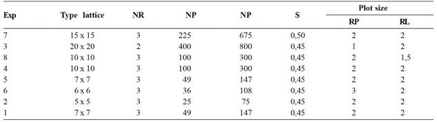
Data on yield (g/plot) of eight experiments in the square lattice design were analyzed (Table 1).

Table 1:
Description of experiments to evaluate bean yield: type of lattice, number of repetitions (r), number of progeny (P), total number of plots (NP), spacing (E), number of rows per plot ( L), row length (C) in meters

Data on spacing between rows and plot size were used to obtain the coordinates relative to the center of each plot within the experimental area. Plot locations are important information required for the spatial statistical analysis.

The position of each plot in the experimental grid was determined by the coordinates L and C, relative to the center of the plots: coordinate L in the width direction and coordinate C in the length direction. Thus, the distance between the plots i and j was obtained by:

h = [(L_j - l_i)² + (C_j - C_i)²]^0.5

L_j is the ordinate related to the width in the plot j;

L_i is the ordinate related to the width in the plot i;

C_j is the abscissa related to the length in the plot j; and

C_i is the abscissa related to the length in the plot i.

Data on bean yield were statistically analyzed assuming independent errors (usual analysis), and considering the spatial dependence of errors (spatial analysis).

The analysis of data with independent errors (usual analysis) used the following models:

Model 1 (lattice analysis): y_ijk = μ + r_k + b_j(k) + p_i + e_ijk where:

y_ijk is the value observed for yield of progeny i, in block j within repetition k;

μ is the constant associated with all observations;

r_k is the fixed effect of repetition k;

b_j(k) is the fixed effect of block j within repetition k;

p_i is the fixed effect of progeny i;

e_ijk are the random errors associated with the observations, assuming independence of errors.

Model 2 (analysis in randomized complete blocks): y_ik = μ + r_k + p_i + e_ik where:

y_ik is the value observed for yield of progeny i, within repetition k.

While the analysis with dependent errors (spatial analysis) used the following model:

Model 3 (dependent errors and analysis in randomized complete blocks): y_ijk = μ + r_k + p_i + e_ijk where:

e_ijk are the random errors associated with observations, assuming dependence of errors. The other terms of the models 2 and 3 were defined as in model 1.

The experiments were arranged in the lattice design, but there were two types of analyses: one in lattice and another in blocks. The errors estimated in both lattice and randomized blocks analyses were tested for the existence of spatial dependence and fitting of the geostatistical models.

Initially the spatial dependence was evaluated with the Durbin-Watson test (1950), which tests the hypothesis of zero autocorrelation (H₀: ρ = 0) .The statistic (d) of the DW test is defined by:

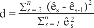
Where,

s = 1, 2, 3, ..., n, the order of the plot location in the experiment, associated with the residue ê_s, and this order had obeyed successive numbering of the plots, so ê_s and ê_s-1 indicate errors from adjacent plots.

The relationship between d and ρ ιs approximately given by d = 2(1 - ρ) .Thus, if there is spatial autocorrelation (ρ = 0), the expected value for the statistic d is 2: values ​​for d significantly smaller than 2 indicate positive autocorrelation; and values ​​significantly greater than 2 indicate negative autocorrelation (Reis & Miranda Filho, 2003).

The spatial dependence was also graphically analyzed through empirical semivariograms that show the behavior of semivariances between errors due to the distance (h), between plots. The semivariance was estimated by the following equation:

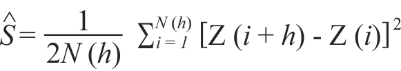
Where,

N(h) is the number of error pairs separated by the distance h, Z(i) and Z(i + h) are estimates of errors relative to the plots i and i + h separated by the distance h.

From the estimated semivariances, the theoretical semivariogram were fitted using the geostatistical models, with and without nugget effect, to describe the spatial variability of errors in the analyses in lattice and in blocks, estimating the parameters contribution (C), range (a), and nugget effect C₀. When S(0) ≠ 0, a new term appears in the semivariogram, the nugget effect C₀ and in this case, the threshold is given by C+C_0, where C is the contribution which is the difference between the threshold and the nugget effect. The stabilization of the observations at a certain distance is called range (a) and all values ​​above the range have random distribution, therefore, independent from each other (Guimaraes, 2004).

The geostatistical models fitted, with nugget effect, are described below:

Exponential model: S(h) = C₀ + C[1 - e^(-3h/a)], where d is the maximum distance between plots in which the semivariogram is defined;

Spherical model: S(h) = C₀ + C[1.5(h/a) - 0,5(h/a)³], for 0 < h < a;

Gaussian model: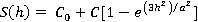, for 0 ≤ h ≤ d.

The degree of spatial dependence (GD) was estimated as a function of the parameters estimated for the theoretical semivariogram, nugget effect (C₀) and threshold (C + C₀) according to Guimaraes (2004):

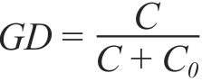
The following spatial dependence classes were adopted:

i) Strong, if 0.75 < GD < 1;

ii) Moderate, if 0.25 < GD < 0,75 and

iii) Weak, if GD > 0.25.

Two structures were considered for the matrix of residual variances and covariances (R):

i) R = IC (for models 1 and 2, independent errors)

ii) R = IC₀ + FC (for model 3, dependent errors), where I is the identity matrix, C is the residual variance in the model with independent errors and the contribution parameter in the model with dependent errors, C₀ is the nugget effect and F is the matrix formed by the elements of the distance function f(h). This function corresponds to the geostatistical models used to fit the theoretical semivariogram.

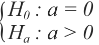
The likelihood ratio test (LRT) was used to compare the models with independent errors (models 1 and 2) with the model for spatially dependent errors (model 3), respectively, the reduced model (a = 0) and the complete model (a > 0). This comparison is to test the significance for the parameter range (a):

Under normal data, the statistic of LRT test has approximately a chi-square distribution with v degrees of freedom given by:

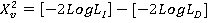
Where,

LogL is the maximum point for the logarithm of the residual likelihood function for the reduced model with independent errors (I) and complete model with dependent errors (D), the degree of freedom v is obtained from the difference between the number of parameters of the complete model and reduced model (Duarte, 2000).

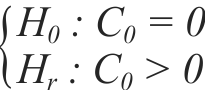
The LRT test was also used to compare the models with and without nugget effect, and a test for significance of the parameter nugget effect (C₀) as follows:

The quality of fit of the models was evaluated by the Akaike Information Criterion (AIC), which penalizes models with large number of parameters (p). It is considered the most parsimonious model, one that had the lowest absolute value for this criterion. The AIC is given by:

AIC = -2LogL + 2p,

Where,

p is the number of estimated parameters and logl the logarithm of the maximum of the likelihood function (Akaike, 1973).

SAS procedures (SAS, 2003) were used for the Durbin-Watson test (proc autoreg), to calculate semivariances and generate empirical semivariograms (proc variogram) to fit the geostatistical models and the analyses of the models with independent and dependent errors (proc mixed).

RESULTS AND DISCUSSION

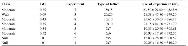
In the analysis of randomized blocks, six of the eight experiments evaluated showed spatial dependence of errors: one with weak dependence and five with moderate dependence, according to the intervals of the degree of dependence estimated (Table 2). Thus, in experiments with spatial dependence, the selection of bean progenies will be more efficient with methods that take into account the spatial variability of errors.

Table 2:
Class and spatial dependence degree (GD) estimated in the experiments, type of lattice, and size of experiments of bean yield evaluation, in randomized blocks analysis

Duarte & Vencovsky (2005) evaluated the classification of soybean genotypes, and found a coincidence of only 46% between the two statistical analysis models, spatial and non-spatial. Storck et al. (2011) also found similar results for 26 competition trials of bean cultivars. In these trials, the selective accuracy increased on average from 0.82 to 0.89 by using the Papadakis method, which is one of the spatial analysis methods that uses the errors of neighboring plots as a covariate to perform a more effective control of the spatial variability.

However, experiments with no or weak spatial dependence do not require spatial analysis methods.

The spatial analysis of Papadakis and moving means has not improved the experimental precision of sugarcane genotype evaluation (Candido et al., 2009). In selection trials of clones of orange cv. Pera, autoregressive models to describe the spatial dependence of errors provided small gains in quality of fit in comparison with the randomized blocks analysis (Maia et al., 2013). The authors explained the results were probably due to the absence of spatial dependence in the evaluated trials.

Yang et al. (2004) analyzed data from 157 trials of pear varieties, and found that the efficiency of the spatial analysis was higher in trials where the blocks were large and with great number of varieties evaluated, probably because of the greater heterogeneity within blocks. Costa et al. (2005) also argued that it is expected that in experiments with greater heterogeneity intrablock, the use of spatial analysis becomes more efficient.

However, in this study there was no relation between the size of the experiments and the spatial dependence of errors. For example, experiments 1, 2, 5 and 6 had similar sizes, ranging from 25 to 49 progenies, but nonetheless, the first two experiments had no spatial dependence and the others had moderate spatial dependence (Table 2). The experiment 7, though with the largest size, had estimated spatial dependence weak to moderate, with degree of dependence of 0.25, which was lower than the degree of dependence of the much smaller experiments 5 and 6 (Table 2).

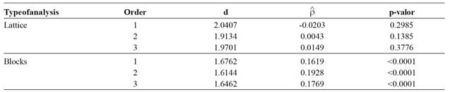
The results of the spatial dependence of the experiment 7 are shown in Tables 3, 4 and 5, whereas the results of other experiments are described in the text.

Experiment 7 was installed in a 15x15 lattice to evaluate 225 progenies, and occupied an area of ​​approximately 1,800 m². In the lattice analysis of this experiment, the statistic d of the DW test for the spatial autocorrelation between errors, from the 1^st to the 3^rd order, ranged from 1.9134 to 2.0407, with p-values of 0.2985, 0.1385 and 0.3776, respectively (Table 3), indicating zero autocorrelation or independence between errors. However, in the randomized blocks, the statistic d ranged from 1.6144 to 1.6762, indicating significant spatial autocorrelation (p <0.0001) of 1^st, 2^nd and 3^rd order estimated 0.1619, 0.1928 and 0.1769, respectively. This result shows the spatial dependence of the estimated errors only in the randomized blocks analysis.

Table 3:
Result of Durbin-Watson test for significance of spatial autocorrelation from 1^st to 3^rd order, between errors estimated in the lattice and randomized blocks analyses for bean yield of experiment 7

• = spatial autocorrelation estimated; d = statistic of the Durbin-Watson test.

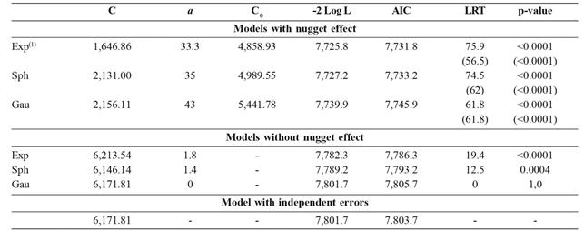
Comparing the fitted models, the LRT test (Table 4) showed that in the randomized blocks analysis, models with dependent errors, with and without nugget effect (C₀), differed significantly (p0.0004) from the model with independent errors, except for the Gaussian model without nugget effect. The same test (LRT), comparing models with and without nugget effect, showed that models with nugget effect were the most suitable, since this parameter was significant (p <0.0001).

Table 4:
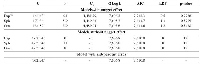
Estimates of the parameters contribution (C), range (a) and nugget effect (C₀), maximum value for the logarithm of the likelihood function (-2 Log L), Akaike Information Criterion (AIC), statistic the likelihood ratio test LRT of for the comparison between geostatistical models, with and without nugget effect, compared to the model with independent errors, in the randomized blocks analysis of the experiment 7

• ¹
  Geostatistical models: Exp= Exponential, Esph= Spherical, Gau = Gaussian.

The estimates for the parameter range, in the randomized blocks analysis ranged from 33.3 to 43 m (Table 4). According to the AIC criterion and the LRT test, the exponential model with nugget effect was the most appropriate to consider the spatial dependence of errors, with the following estimates for the parameters contribution (C), range (a) and nugget effect (C₀), 1,646.86; 33.3 and 4,858.93, respectively (Table 4). These results show that plots separated by distances shorter than 33.3 m present dependent errors, and also that the error variance is dependent on the distance between plots, so that their location contributes to an increase in error variance of up to 1,646.86. Costa et al. (2005) found no significant differences between the spherical, exponential and Gaussian models for the estimates of variance components. However, Duarte & Vencovsky (2005), evaluating the efficiency of spatial statistical analysis in the selection of soybean genotypes, found similar results to those of experiment 7, significant spatial autocorrelation by the DW test, and best fit for the exponential model with a range of 20.4 m. In the study of Negash et al. (2014), the exponential model also showed the best quality fit for most of the evaluated trials.

The lattice analysis of experiment 7 found range estimates of zero or close to zero and non-significant LRT test (p> 0.01), indicating that the models with dependent errors were not different from the model with independent errors (Table 5), which characterizes spatial independence of errors in the lattice analysis.

Table 5:
Estimates of the parameters contribution (C), range (a) and nugget effect (C₀), maximum value for the logarithm of the likelihood function (-2 Log L), Akaike Information Criterion (AIC), statistic the likelihood ratio test LRT of for the comparison between geostatistical models, with and without nugget effect, compared to the model with independent errors, in the lattice analysis of the experiment 7

• ¹
  Geostatistical models: Exp= Exponential, Sph= Spherical, Gau = Gaussian.

Similarly, Costa et al. (2005) also concluded that the spatial analysis did not improve the accuracy of experiments of evaluation of bean and corn progenies, in lattice analysis. The authors did not test the spatial dependence of errors, but probably the errors estimated in the lattice analysis did not show spatial dependence, which explains the results.

Negash et al. (2014) pointed out that the advantages and validity of using spatial analysis methods depend on the existence of spatial dependence. In some trials, they found that the traditional analysis was more efficient than spatial analysis.

In experiment 1, in a 7x7 lattice, the statistic d DW test for spatial autocorrelation between errors, from 1^st to 3^rd order, showed values very close ​​to 2 for the lattice analysis with p-values ​​of 0.0728, 0.2236 and 0.2590, indicating non-significant autocorrelation (p> 0.01). In the randomized blocks analysis, the estimates for statistic d ranged from 1.6727 to 1.8608 with p-values ​​of 0.1987, 0.0432 and 0.0334, also indicating non-significant spatial autocorrelation (p> 0.01). These results show that for Experiment 1, the estimated errors in both the lattice and randomized blocks analyses are independent, i.e., no spatial dependence. The LRT test also showed non-significant result, which characterizes spatial independence of errors (p> 0.01).

Experiment 2, in a 5x5 lattice, showed structure of spatial dependence similar to those of experiment 1. The DW test found non-significant autocorrelation for the estimated errors in the lattice and randomized blocks analyses. In the randomized blocks analysis, the LRT test for exponential, spherical and Gaussian models with nugget effect showed p-values ​​of 0.1572, 0.1353 and 0.1422, respectively, and for the models without nugget effect, the p-values ​​were 0.0483, 0.0614 and 0.0613, respectively. Thus, the models with dependent errors were not significantly different from the model with independent errors.

In experiment 3, in a 20x20 lattice, the estimated errors in the lattice analysis were randomly distributed in the experimental area, according to the DW test for spatial autocorrelation. The spatial autocorrelations were not significant with p-values ​​of 0.2164, 0.1909 and 0.4502 for the 1^st, 2^nd and 3^rd orders, respectively. In the randomized blocks analysis, the spatial autocorrelations were also non-significant at 1% probability with p-values ​​of 0.0141, 0.1418 and 0.0609, indicating independence of errors. The LRT test, in the block analysis, found that the exponential, spherical and Gaussian models with nugget effect, were significantly different from the reduced model with independent errors (p <0.0001). Therefore, the range was significantly different from zero, showing that the errors had spatial dependence. The nugget effect was also significant (p <0.0001). The AIC test and previous results showed that the most suitable geostatistical model to analyze experiment 3, in randomized blocks analysis, was the Gaussian model with nugget effect with the following estimated parameters (C = 125.98, a = 5.9 and C₀ = 1,216.61). Thus, all errors associated with plots with distance shorter than 5.9 m are correlated. Estimates of the Gaussian model parameters were used to calculate the spatial dependence of errors (GD), indicating weak spatial dependence (GD = 0.09). Contradictory results of DW and LRT tests appeared only in experiment 3. The DW test showed that the errors were not spatially correlated, while the LRT test showed that the range and the nugget effect were significant, although the spatial dependence was weak.

In the experiment 4, in a 10x10 lattice, the statistic d of the DW test for spatial autocorrelation between errors in the lattice analysis, were close to 2 with p-values ​​of 0.4385, 0.3503 and 0.0757, indicating that the errors are spatially independent. However, in the randomized blocks analysis, the autocorrelation was significant (p <0.0002), indicating that errors are correlated up to the 3^rd order, with estimated ​​ autocorrelation values of 0.3020, 0.2847 and 0.2070 for 1^st, 2^nd and 3^rd orders, respectively. Thus, it is characterized independence of errors in the lattice analysis and spatial dependence in the randomized blocks analysis for experiment 4. The LRT test showed that in the randomized blocks analysis the models with dependent errors (with or without nugget effect) differed from the reduced model with independent errors (p <0.0001), except for the Gaussian model without nugget effect. Estimates of the range for the randomized blocks analysis varied between 1.5 and 18.1 m. According to the AIC criterion and the results of the LRT test, the Gaussian model with nugget effect was the most appropriate, the following estimates for the parameters (C = 2657.42, a = 9.6 and C0 = 4899.60), which reflects moderate spatial dependence (GD = 0.35). In the analysis in lattice all geostatistical models, with and without nugget effect did not differ from the reduced model with independent errors, indicating that the analysis in lattice ensured the independence of the errors.

In experiment 5, in a 7x7 lattice, the results of randomized blocks analysis were similar to experiment 4, with moderate spatial dependence (GD = 0.34), but the exponential model did not show the best fit. Also, according to the AIC criterion, the Gaussian model with nugget effect was the most suitable for the randomized blocks analysis with the estimated parameters C = 1,415.70, a = 7.2 and C₀ = 2,629.69. For the lattice analysis, all models, with and without nugget effect, were not different from the model with independent errors, indicating that the lattice analysis ensured the independence of errors.

In experiment 6, in a 6x6 lattice, there was spatial autocorrelation of 1^st order (p <0.001) in the randomized blocks analysis, with estimated value of 0.367; and 2^nd order, with estimated value of 0.201. The LRT test showed that the range was significant (p <0.0004) for all models, with and without nugget effect, and the nugget effect was significant for the spherical and Gaussian models with p-values of ​​0.003 and 0.004, respectively, and non-significant for the exponential model with p-value of 0.2059. The most suitable models for the randomized blocks analysis were: exponential without nugget effect, spherical with nugget effect, and Gaussian with nugget effect. All models showed very similar values, but according to the AIC criterion, the spherical model was the most suitable for the randomized blocks analysis with the estimated parameters (C = 5,191. 76, a = 6.8 and C₀ = 4,738.01), with moderate spatial dependence (GD = 0.52). For the lattice analysis, all models, with and without nugget effect, were non-significant (p> 0.05), indicating independence of errors.

In experiment 8, in a 10x10 lattice, considering the randomized blocks analysis, the DW test indicated significant 1^st order spatial autocorrelation (p <0.001), with estimated value of 0.324. The LRT test showed that in the randomized blocks analysis, the models with dependent errors, with or without nugget effect, differed from the model with independent errors (p <0.0001). The same test, comparing the models with and without nugget effect, showed that the models Gaussian with nugget effect, and exponential and spherical without nugget effect were the most suitable. According to the AIC criterion, the Gaussian model was the most suitable, with the estimated parameters (C = 2,494.34, a = 3 m and C₀ = 3,213.23), and moderate spatial dependence (GD = 0.43).

The lattice analysis for experiment 8 showed spatial autocorrelation of 1^st order of 0.170, and significant by the DW test (p <0.01). The LRT test showed that the geostatistical models differed from the model with independent errors (p <0.008), indicating significant range, with non-significant nugget effect. According to the AIC criterion, the exponential model without nugget effect was the most suitable with the estimated parameters C = 4347.65 and a = 1.7, and moderate spatial dependence (GD = 0.43). Thus, spatial dependence was characterized in experiment 8, for both analyses, block and lattice.

Therefore, the evaluation of the spatial dependence of errors in the eight experiments of genetic evaluation of bean yield found that the use of spatial analysis is required in the experiments 4, 5, 6, 7 and 8. In the other experiments, since the spatial dependence was zero or weak, the spatial analysis does not contribute to increase the experimental accuracy and hence does not increase the efficiency of progeny selection.

Thus, for the analysis of data from experiments 4, 5, 6, 7 and 8, or future experiments installed in the same area we can recommend two alternatives. Lattice analysis for independent errors (model 1) or randomized blocks analysis for dependent errors (model 3), which considers the spatial dependence of errors using the exponential, spherical or Gaussian models to describe the spatial variability of errors. The advantage of the spatial analysis is that in situations with restrictions on the establishment of experiments in lattice, it would be possible to install the experiment in randomized blocks and perform the analysis using geostatistical models to consider the spatial dependence of the errors.

CONCLUSIONS

Weak to moderate spatial dependence of errors was identified in lattice experiments for yield evaluation of bean progenies analyzed in randomized blocks. However, the lattice analysis was effective to ensure the independence of errors in most experiments.

The geostatistical models spherical, exponential and Gaussian, with nugget effect, were efficient to characterize the spatial structure of errors estimated in the randomized blocks analysis, which is an alternative analysis when there are restrictions to the installation of lattice experiments.

AKNOWLEDGEMENTS

The authors would like to express their sincere thanks to the reviewers for their suggestions and criticisms which greatly contributed to improving the quality of this scientific work.

REFERÊNCIAS

• Akaike H (1973) Information theory as an extension of the maximum likelihood principle. In: International Symposium on Information Theory, Budapest. Proceedings, Akadêmia Kiadó. p.267-281.
• Barbosa FR & Gonzaga ACO (2012) Informações técnicas para o cultivo do feijoeiro comum na Região Central-Brasileira: 2012-2014. Santo Antônio de Goiás, Embrapa Arroz e Feijão. 248p. (Documentos, 272).
• Conagin A,Ambrosano GMB & Nagai V (1997) Poder discriminativo da posição de classificação e dos testes estatísticos na seleção de genótipos. Bragantia, 56:403-417.
• Candido LS, Perecin D, Landell MGA & Pavan BE (2009) Análise de vizinhança na avaliação de genótipos de cana-de-açúcar. Pesquisa Agropecuária Brasileira, 44:1304-1311.
• Costa JR, Bueno Filho JSS & Ramalho MAP (2005) Análise espacial e de vizinhança no melhoramento genético de plantas. Pesquisa Agropecuária Brasileira , 40:1073-1079.
• Duarte JB (2000) Sobre o emprego e a análise estatística do delineamento em blocos aumentados no melhoramento genético vegetal. Tese de Doutorado. Escola Superior de Agricultura "Luiz de Queiroz" , Piracicaba . 293p.
• Duarte JB & Vencovsky R (2005) Spatial statistical analysis and selection of genotypes in plant breeding. Pesquisa Agropecuária Brasileira , 40:107-114.
• Durbin J & Watson GS (1950) Testing for serial correlation in least squares regression. Biometrika, 37:409-428.
• Guimarães EC (2004) Geoestatística básica e aplicada. Uberlândia, UFU. 78p.
• Maia E, Siqueira DL, Carvalho AS, Peternelli LA & Latado RR (2013) Aplicação da análise espacial na avaliação de experimentos de seleção de clones de laranjeira Pêra. Ciência Rural, 43:08-14
• Negash AW, Mwambi H, Zewotir T & Aweke G (2014) Mixed model with spatial variance-covariance structure form accomodating of local stationary trend and its influence on multi-environmental crop variety assessment. Spanish Journal of Agricultural Research, 12:195-205.
• Pimentel Gomes F (1990) Curso de estatística experimental. 13ª ed. Piracicaba, Nobel/USP-ESALQ. 468p.
• Reis AJS & Miranda Filho JB (2003) Autocorrelação espacial na avaliação de composto de milho para resistência à largata do cartucho (Spodoptera frugiperda). Pesquisa Agropecuária Tropical, 33:65-72.
• Resende MDV, Thompson R & Welham S (2006) Multivariate spatial statistical analysis of longitudinal data in perennial crops. Revista de Matemática e Estatística, 24:147-169.
• Richetti A & Melo CLP (2014) Viabilidade econômica da cultura do feijão-comum, safra da seca de 2015, em Mato Grosso do Sul. Dourados, Embrapa agropecuária Oeste. 9p. (Comunicado técnico, 197).
• SAS Institute Inc. (2003) Statistical Analysis System user´s guide. Version 9.2. Cary, Statistical Analysis System Institute. 202p.
• Silva CL (2005) Recomendação de Cultivares de Feijão Vermelho para o Estado de Minas Gerais. Dissertação de Mestrado. Universidade Federal de Viçosa, Viçosa. 77p.
• Storck L, Ribeiro ND & Filho AC (2011) Precisão experimental de ensaios de feijão analisada pelo método de Papadakis. Pesquisa Agropecuária Brasileira , 46:798-804.
• Yang RC, Ye TZ, Blade SF & Bandara M (2004) Efficiency of spatial analyses of field pea variety trials. Crop Science, 44:49-55.
• Yang RC & Juskiw P (2011) Analysis of covariance in agronomy and crop research. Canadian Journal of Plant Science, 91:621-641.
• Yates FA (1936) A new method of arranging variety trials involving a large number of varieties. Journal of Agricultural Science, 26:424-455.
• Zanão Júnior LA, Lana RMQ, Zanão MPC & Guimarães EC (2010) Variabilidade espacial de atributos químicos em diferentes profundidades em um latossolo em sistema de plantio direto.Revista Ceres, 57:429-438.
• Zimmerman DI & Harville DA (1991) A random field approach to the analysis of field-plot experiments and other spatial experiments. Biometrics, 47:223-239.

Publication Dates

• Publication in this collection
  Jul-Aug 2016

History

• Received
  16 Sept 2014
• Accepted
  08 Mar 2016