INCLUDING RISK IN ECONOMIC FEASIBILITY ANALYSIS:A STOCHASTIC SIMULATION MODEL FOR BLUEBERRY INVESTMENT DECISIONS IN CHILE

INCLUYENDO EL RIESGO EN EL ANÁLISIS DE VIABILIDAD ECONÓMICA:UN MODELO DE SIMULACIÓN ESTOCÁSTICA PARA DECISIONES DE INVERSIÓN EN ARÁNDANOS EN CHILE

ABSTRACT

The traditional method of net present value (NPV) to analyze the economic profitability of an investment (based on a deterministic approach) does not adequately represent the implicit risk associated with different but correlated input variables. Using a stochastic simulation approach for evaluating the profitability of blueberry (Vaccinium corymbosum L.) production in Chile, the objective of this study is to illustrate the complexity of including risk in economic feasibility analysis when the project is subject to several but correlated risks. The results of the simulation analysis suggest that the non-inclusion of the intratemporal correlation between input variables underestimate the risk associated with investment decisions. The methodological contribution of this study illustrates the complexity of the interrelationships between uncertain variables and their impact on the convenience of carrying out this type of business in Chile. The steps for the analysis of economic viability were: First, adjusted probability distributions for stochastic input variables (SIV) were simulated and validated. Second, the random values of SIV were used to calculate random values of variables such as production, revenues, costs, depreciation, taxes and net cash flows. Third, the complete stochastic model was simulated with 10,000 iterations using random values for SIV. This result gave information to estimate the probability distributions of the stochastic output variables (SOV) such as the net present value, internal rate of return, value at risk, average cost of production, contribution margin and return on capital. Fourth, the complete stochastic model simulation results were used to analyze alternative scenarios and provide the results to decision makers in the form of probabilities, probability distributions, and for the SOV probabilistic forecasts. The main conclusion shown that this project is a profitable alternative investment in fruit trees in Chile.

Index terms
Random values; value at risk; probabilistic forecasts

RESUMEN

El método tradicional de valor presente neto (VPN) que se utiliza para evaluar la rentabilidad económica de una inversión no representa adecuadamente el riesgo implícitoasociado a diferentes variables de entrada cuando entre ellas se encuentran correlacionadas. Utilizando un enfoque de simulación estocástica para evaluar la rentabilidad del arándano ( LVaccinium corymbosum.) en Chile,el objetivo de este trabajo es ilustrar cuán compleja se torna la evaluación económica cuando la rentabilidad del proyecto depende de variados riesgos que se encuentran correlacionados. Los resultados delanálisis de simulación sugieren que no incluir la correlación intra-temporal entre las variables de entrada lleva a subestimar el riesgo de inversión. La innovación metodológica de este trabajo ilustra la complejidad de las interrelaciones entre variables inciertas y sus impactos sobre la conveniencia de llevar a cabo este tipo de negocios en Chile. Los pasos para realizar el análisis de viabilidad económica fueron: Primero, se ajustaron distribuciones de probabilidad para las variables aleatorias de entrada (SIV), las cuales fueron simuladas y validadas. Segundo, los valores aleatorios de las SIV fueron utilizados para calcular valores aleatorios de variables como producción, ingresos, costos, depreciación, impuestos y flujos netos de caja. Tercero, el modelo estocástico completo fue simulado con 10.000 iteraciones utilizando valores aleatorios para las SIV. Este resultado entregó información para estimar las distribuciones de probabilidad de las variables estocásticas de salida (SOV) tales como el valor presente neto, tasa interna de retorno, valor en riesgo, costo medio de producción, margen de contribución y rentabilidad sobre capital. Cuarto, los resultados de la simulación del modelo estocástico completo fueron utilizados para analizar escenarios alternativos y proveer los resultados a los tomadores de decisión en la forma de probabilidades, distribuciones de probabilidad y pronósticos probabilísticos para las SOV. La principal conclusión muestra que este proyecto es una alternativa de inversión rentable en árboles frutales en Chile.

Index terms
Valores aleatorios; valor en riesgo; pronósticos probabilísticos

INTRODUCTION

Interest in stochastic analysis by Monte Carlo simulation in the agricultural sector has been growing during the last 15 years (RICHARDSON et al., 2000; BEWLEY et al., 2010). The traditional measure of the profitability using the net present value (NPV) under a deterministic approach can lead to deception because it does not adequately represent the implicit risk associated with input variables. It is very important to provide historical information to adequately characterize the implied risk, and even relevant market information. In some cases it is possible to seek the opinion of experts as a first-bestpresumption as to how it could the likelihood of occurrence of a particular event be. This last aspect is a formalization of what happens many times in real life, where administrators resort to experts to consider different scenarios about what will happen with a particular investment. This study develops a model that allows the evaluation of interactions between bio-technical (such as production) and economic (such as price and exchange rate) variables and their relationship with investment decision-making for the particular case of blueberry growing (Vaccinium corymbosum L.) in Chile. Thus, a stochastic simulation model is considered as a tool of dynamic financial analysis that takes into account a proper structure of dependencies and correlations between stochastic input variables -SIV (EMBRECHTS et al., 2002) to evaluate the risk associated to the fruit business. These relationships are presented using an intra-temporal correlation matrix (RICHARDSON et al., 2000; BLUM; DACOROGNA, 2004) for improve the estimation of the risk of the business.

Some studies on cost-benefit analysis in the fruit sector indicate that, in general, fruit growing is a profitable activity (KREUZ, 2002; ;LOBOS & MUÑOZ, 2005 UZUNÖZ; AKÇAY, 2006).

A computer system is delivered to assess the economic viability of a fruit plantation when there is a set of underlying variables to the model that are uncertain. This study illustrates the complexity of the interrelationships between uncertain variables and their impact on the convenience of carrying out this type of business in Chile. Although the process for the final decision will depend on the particular behavior of the decision maker against the risk, especially when it is considered that the majority of farmers are averse to risk, as suggested by the national and international literature (TOLEDO; ENGLER, 2008; HOWLEY; DILLON, 2012; KHAN et al., 2013). Thus, the objective of this study is to describe a dynamic simulation model developed to examine the economic results of the investment in blueberries (Vaccinium corymbosum L.).

MATERIAL AND METHODS

Description of the stochastic simulation model

RICHARDSON et al. (2007) proposed four steps to perform an analysis of economic viability based in a Monte Carlo simulation model. First, it must be defined the probability distribution for all the stochastic input variables (SIV), the respective parameters must be obtained, then they must be simulated and, finally, validated. Second, the SIV random values are used in accounting identities to calculate random values of variables such as production, revenues, costs, depreciation, taxes and net cash flows. Third, the complete stochastic model is simulated many times (i.e. 10,000 iterations) using random values for the SIV. The result of the 10,000 iterations contains information that is used to estimate the probability distributions for unobservable stochastic output variables (SOV) such as Net Present Value (NPV), Internal Rate Return (IRR) and Value-at-Risk, known as VaR (MANOTAS & TORO, 2009). Fourth, the project analyst uses the results of the simulation of the complete stochastic model to analyze various alternative scenarios and provide the results to decision makers in the form of probability distribution and probabilistic forecasts for the SOV.In this study a systemic and dynamic stochastic simulation model was developed to evaluate the economic performance of the crop of highbush blueberry (Vaccinium corymbosum L.) and rabbit-eye blueberry (Vaccinium ashei Reade). The model incorporates the correlations between the SIV so as not undervalue the exposure to risk faced by farmers, since the usual positive correlation between the input random variables normally implies that the resulting distributions have higher probability in the tails of these distributions. The model was designed to characterize the productive and economic complexities of a plantation of blueberries in Chile, including the interdependencies between random variables through statistical adjustments. The basic deterministic model was built in Microsoft Excel 2007 (Microsoft, Seattle, Washington). @Risk5.7 (Palisade Corporation, Ithaca, New York) was used to incorporate the stochastic nature of the critical variables.The modeling process began with the definition of a set of inputs to describe the initial situation and the behavior of blueberry planting.The behavior of the plantation was represented using technical-economic coefficients obtained from historical records of blueberry plantations located in the Center-South zone of Chile. The historical values of critical variables and values obtained from the opinion of experts were incorporated into the system using parametric and non-parametric probability distributions, respectively. Both types of variables were added as inputs to the model. The flexibility of this model lies in the manipulation of the inputs that describe the initial situation and the characteristics of the plantation and the potential impact of the stochastic simulation on the economic viability of this type of business.After entering the set of coefficients and input variables the estimates were done by measuring the impact on the economic viability of the plantation.Changes over a 10 year horizon for their respective coefficients and stochastic input variables were analyzed. The intra-temporal relation affecting such estimates were also included as input. As a result, flows of income and random costs that were used to obtain economic viability indicators of the plantation project were obtained. Additionally, an advanced sensitivity analysis was performed on some deterministic variables and an analysis of stress was carried out upon the main stochastic variables.

Stochastic variables

There is a wide literature on high volatility in products and agricultural commodities markets (BUGUK et al., 2003; SEKHAR, 2004; ALI & GUPTA, 2007; WILLIAM & DAHL, 2009). As a result of this volatility, economic conditions and profitability of agricultural investments can vary considerably depending on the prices paid for inputs and the prices received by the outputs generated by the project. In a Monte Carlo simulation approach stochastic variables are those variables that the decision maker cannot foresee with certainty. These variables have two components: a deterministic component, whose prediction can be made with certainty, and a stochastic component, whose prediction cannot be made with certainty.The stochastic variables used in the model developed in this study include the average weekly price of blueberries ( Pt ), the annual production of rabbit-eye and highbush blueberry (Qit), and the monthly real exchange rate (Tt ). The Qit was simulated using the multivariate empirical (MVE) distribution described by RICHARDSON et al. (2000) to account for correlation among the variables.

Historical data of the period 2000/01 to 2010/11were used to estimate the parameters for the MVE distribution. Thus Q1t is rabbit-eye blueberry and Q2t is highbush blueberry, for t = 1,2,...10 . An intratemporal correlation matrix of the two simulated production was incorporated in the simulations to account for correlations among production within a given year in each simulation. In this correlation analysis blueberry stochastic price and real stochastic exchange rate was not included because it is assumed that the production of each individual producer does not affect the price or exchange rate they pay or receive.There are two ways to remove the random component of a stochastic variable: use regression analysis to estimate the systematic variability xit, or use the mean when there is no systematic variability.

In this last case xit = xi for each random variable xi and each year t.

Step 1. Following RICHARDSON et al. (2000), the first step in estimating the parameters for a MVE distribution is to separate the random and non-random components for each of the stochastic variables. In this study, regression analysis was used to identify the deterministic component of each random variable, as shown in equation 1.

(1).Deterministic component of historical values (forecast, xit) 1.1 For the stochastic variables P_it and T_it: autoregressive model of order p, or AR(_p) 1.2 For the stochastic variables Q_it: no-lineal mathematical models.

Step 2.The second step is to calculate the random component of each stochastic variable. The random component is simply the residual from the predicted or non-random component of the variable. It is this random component of the variable that will be simulated, not the whole variable, as defined in equation 2.

(2) Random component (residuals, eit) 2.1For each random variable xi and each period t: e_it= x_it - x_itStep 3.The third step in estimating the parameters for a MVE distribution is to convert the residuals in equation 2 to relative deviates about their respective deterministic components (equation 3).

(3) Relative variability (deviates, d_it) 3.1 For each of the periods and for each random variable x_i: d_it = e_it/x_itStep 4.The fourth step is to sort the relative deviates in equation 3.1 and to create pseudominimums (p_min) and pseudo-maximums (p_max) residual terms for each random variable. The relative deviates are simply sorted from the minimum deviate to the maximum to define the points on the cumulative empirical distribution for each random variable x_it. According to Law & Kelton (1991), in a standard empirical distribution the probability of simulating the minimum or maximum of the data is equal to zero. This problem can be corrected by adding two pseudo observations: pmin and pmax values are calculated and added to the data resulting in an (T + 2) - empirical probability distribution point (equation 4).

(4)Relative variability ordered from more to less (sorted deviates, s_it) 4.1 For each random variable : s_it = sorted (dit from min to max) 4.2 pmin_i = minimum s_it . 1.000001 4.3 pmax_i= maximum s_it .1.000001

Step 5. The fifth step is to assign probabilities to each of the sorted deviates in equations 4. The probabilities for the pmin and pmax are defined to be 0.0 and 1.0 to ensure that the process conforms to the requirements for a probability distribution. Each of the observed deviates had an equal chance of being observed in history so in the simulation process that assumption must be maintained (equation 5).

(5) Probabilities of occurrence for the sorted deviates (psit) 5.0 P (pmin_i) = 0.0 5.1 P (s_i1) = ( 1/T) / 2 5.2 P (s_i2) = (1/T) + P ( S_i1) 5.3 (T) p (s_iT) = (1/T) + P (s_i(T-1)5.4 (T+1) P (pmax_i) = 1.0

Step 6.The sixth step is to calculate the M x M intra-temporal correlation matrix for M random variables. The intra-temporal correlation matrix is calculated using the unsorted, random components (eit) from equation 2.1 and is demonstrated for a 2 x 2 matrix.

(6) Intra-temporal correlation matrix for two random variable xi to xj (Eq.01)>

The sixth step completes the parameter estimation for a MVE distribution. The parameters used for simulation are summarized in equation 7.

(7) Parameters used for simulated for random variables,random variables, historical periods, and , simulated period.The completed MVE probability distribution can be simulated in Excel using @Risk to generate independent values that are distributed according to a normal distribution with mean 0 and standard deviation equal to 1.

This study is interested in considering the intra-temporal correlation between two stochastic variable and ten historical periods, i.e. Q_1t y Q_2t for t = 1,2...10. Later, this work is interested in obtaining values fora nine-year simulation period that is Q1k y Q_2t for k = 2,...10. The reason is that a blueberry plantation requires 1 period of establishment (year 0) and another period for the formation of the crop (year 1), starting new production only in the year 2.

In addition, this study was evaluated in a 10 year horizon. As shown by Richardson et al. (2000), prior to simulation, the square root of the intra-temporal correlation matrix must be calculated. The square root procedure for factoring a covariance matrix is used to factor the intra-temporal correlation matrix and is named MSQRT, or R matrix (equation 8.1).

Using Cholesky’s factorization method we can obtain R matrix as = TTT(equation 8.2), where is upper triangular matrix and TT is lower triangular matrix of Cholesky, this last is (equation 8.3).

Then we should generate a simple of independent standard normal deviates (ISND) equal the number of random variables. In this research, 18 ISNDs are needed for two variables and nine simulation years. The result of this process is nine vectors, one for each year of forecast, made up of two variables and two independent values (equation 8.4). The best alternative to the problem of generating ISNDs is to use=RiskNormal (0;1) function of @ Risk to generate the ISNDs and to select the Latin Hypercube option.

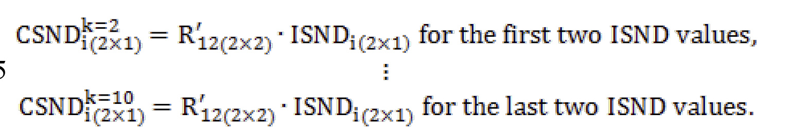
For obtaining the correlated standard normal deviates (CSND) for simulated years 2-10, the matrix multiplication is repeated once for each year to be simulated, using the same matrix R12 each time but a different set of eight ISNDs. The resulting two values in each of nine vectors are intra-temporally CSNDs (equation 8.5). According to RICHARDSON et al. (2000) for large samples (number of iterations) the CSND in equation 8.5 exhibit similar intra-temporal correlation to that observed in the rij(MxM) correlation matrix in equation 7.

(1) Estimating the parameters for a MVE distribution 8.1 matrix: R12(2x2) = MSQRT (p12(2x2)) 8.2 Factorized R matrix by Cholesky’s method: R12(2x2) = TTT 8.3 Lower triangular matrix of Cholesky: = R’12(2x2) = TT 8.4 Vector of ISNDs: ISND18x1 = RiskNormal (0;1) -> nine vector ISND(2x1)

Now we can transform the CSNDs from equation 8.5 (Eq.02) inform deviates.

8.5 -

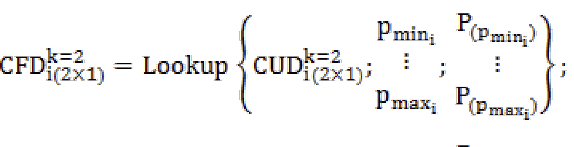
The result of this step allows obtai) ning the correlated uniform deviates (CUDs) (equation 9.1). Using the CUD, along with the respective variable’s and one simply interpolates among the values to calculate a random deviate for variable (equation 9.2).

(9)Estimating CUD and CDF values (Eq.04) , (Eq. 05), (Eq.06). 9.1 -

9.2 -

for the first two CUD values, 9.3 -

for thelast nine CUD values.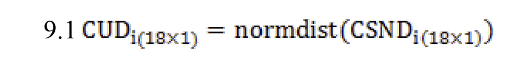

Now we can apply the CFD to their respective projected means. In this case, projected values from the OLS regressions for years 2-10 in equation 1.2.The simulate random values in year k for variable xi is presented in equation 10.

(10)Estimating simulate random values in year k. (Eq.07) 10.1

for the first two CFD variables, (Eq. 08) ,(Eq.09) 10.2

for the second two CFD variables, and 10.3

for the last two CFD variables.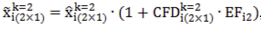

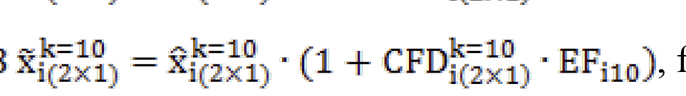
In equation 10 EFik is an expansion factor to allow managing the coefficient of variation over time.

In this research we suppose that EFik = 1.0 (scenario 1) and EFik =1.5 (scenario 2) for all years.

To obtain the net price received by Chilean blueberry producers it was used historical average prices FOB / Chile obtained from the major exporting companies considering the 2005/06 to 2009/10 seasons. This series of weekly prices, including from week 46 of each year until week 13 of the following year, was converted to dollars per kilo of December 2010 using as a deflator the Real Observed Exchange Rate (TCR) index. Then, weekly prices were converted to a stationary series calculating the natural logarithm of differences in the t period [LNPt = LN (Pt/Pt-1)]. The Dickey-Fuller ADF contrasts were used to test stationarity of the series LNPt (DICKEY; FULLER, 1979) and the Phillips-Perron unit root test (PHILLIPS; PERRON, 1988).

Since it was observed that the autocorrelation of the series fade exponentially to zero and the partial autocorrelations are cut, an autoregressive model of order p ––AR(p)- was adjusted considering the series LNPt as the dependent variable in time t and this same variable, but with p lag periods as independent variables: LNPt = f0 + f1LNQt-1+ f2LNPt-2 + ...+fp LNPt-p + et, where fi are the coefficients to be estimated and et is the error term in time t whose assumptions are the same as those of the standard regression model. To determine the number of lags, the number of significant autocorrelations and partial autocorrelations was counted, determining the statistical convenience of adjusting an autoregressive model of order 5 –AR(5)–. To test the relevance of the adjusted model, the Ljung-Box Q statistic was used.

Then, the regression autoregressive equation was used to estimate the value of LNQt expected (forecast) for each year, thus obtaining the continuous expected return (forecast) series with onset in week 47 of the 2005/06 season. The values of the prediction were transformed “backwards” to prices in dollars per kilogram.

Next, residual terms were calculated by dividing the difference between the actual and predicted prices by the predicted price. These residual terms were sorted from smallest to largest and pseudo minimum and pseudo maximum residual terms were calculated by multiplying the smallest and largest residual terms, respectively, by 1.000001. The pseudo minimum and pseudo maximum parameters, the sorted residual terms and their associated cumulative probabilities were incorporated into empirical distributions using the =RiskCumul function of @ Risk. These empirical distributions were used to estimate error terms to account potential variation in prices from expected prices. The deterministic expected price for a given week was set using the blueberry expected price by the autoregressive model estimated. Finally, the simulated error terms were added to the deterministic prices to provide blueberry stochastic prices.

The production data were taken from historical records of different farmlands dedicated to the production of blueberry, rabbit-eye and highbush cultivars, from which a production curve was obtained for each cultivar in a period of 10 agricultural seasons, from 2000/01 to 2009/10.

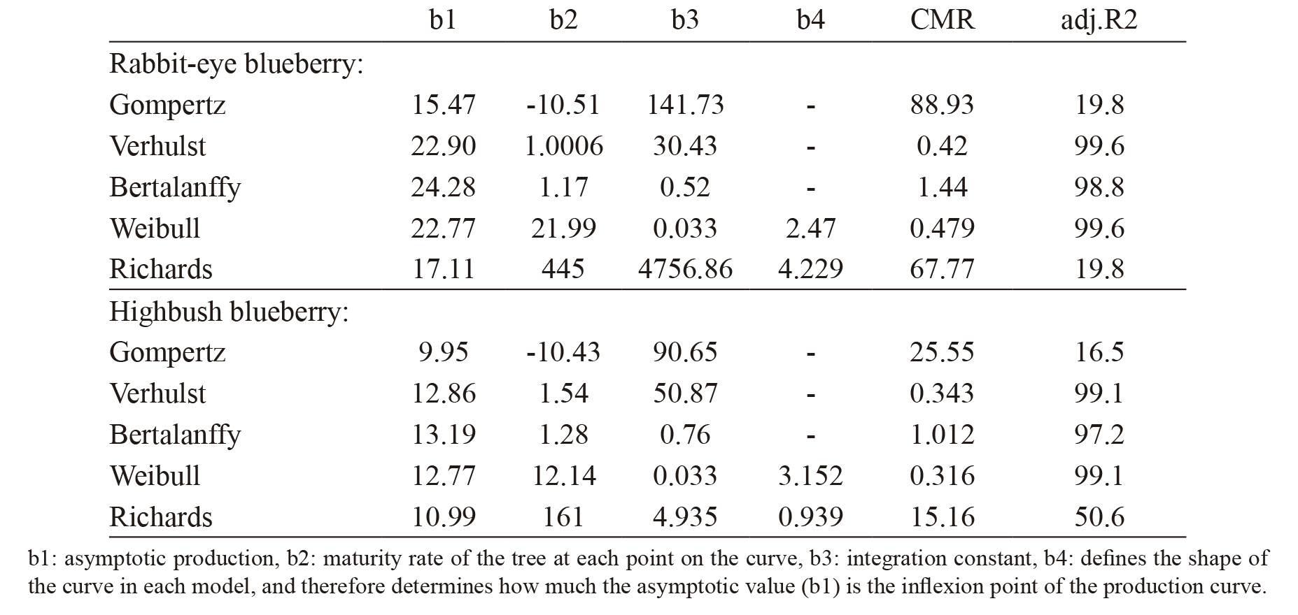
Non-linear mathematical functions proposed byGOMPERTZ (1825), VERHULST (1838), VON BERTALANFFY (1957), WEIBULL (1951) and RICHARDS (1959) were considered to estimate the growth of blueberry production and the parameters of each curve, using Levenberg-Marquardt estimation method of the non-linear SPSS 15.0 procedure. Then, regression equations for each blueberry cultivar were developed to predict production of rabbit-eye blueberry (QR_t) and highbush blueberry (QHt) , both as dependent variable, with 2001 as year 1. In these non-linear functions LNQt was considered as dependent variable and this same variable, but with a lag period (LNQt-1), as independent variable. The goodness of fit of the models was evaluated by the criteria: coefficient of determination (R2 adjusted) and mean square of the residue (CMR).

The function that best described the behavior of the production of rabbit-eye blueberry was theVERHULST (1838) logistic growth curve: yt = b1/(1 + b3 * exp(-b2 * yt-1)) where yt is the production of QRt in the period t and y_t-1 is the laggard production in a period. On the other hand, the function that best described the production behavior of highbush blueberry was the Weibull distribution:y_t = b1-b2 * exp(-b3 * yt-1 ** b4)) where yt represents the QHt production of the period t and y_t-1 is the laggard production in a period. As in the case of blueberries prices, same technique was used to forecast blueberry stochastic production.

The monthly real exchange rate series for the period 2005 to 2010 was included in the model as a stochastic variable. An autoregressive model of order 8 -AR (8)- was estimated through a non-linear process of minimum squares according to the Box- Jenkins methodology (BOX et al., 2007). As in the case of blueberries prices, same technique was used to forecast real stochastic exchange rate.

Technical coefficients

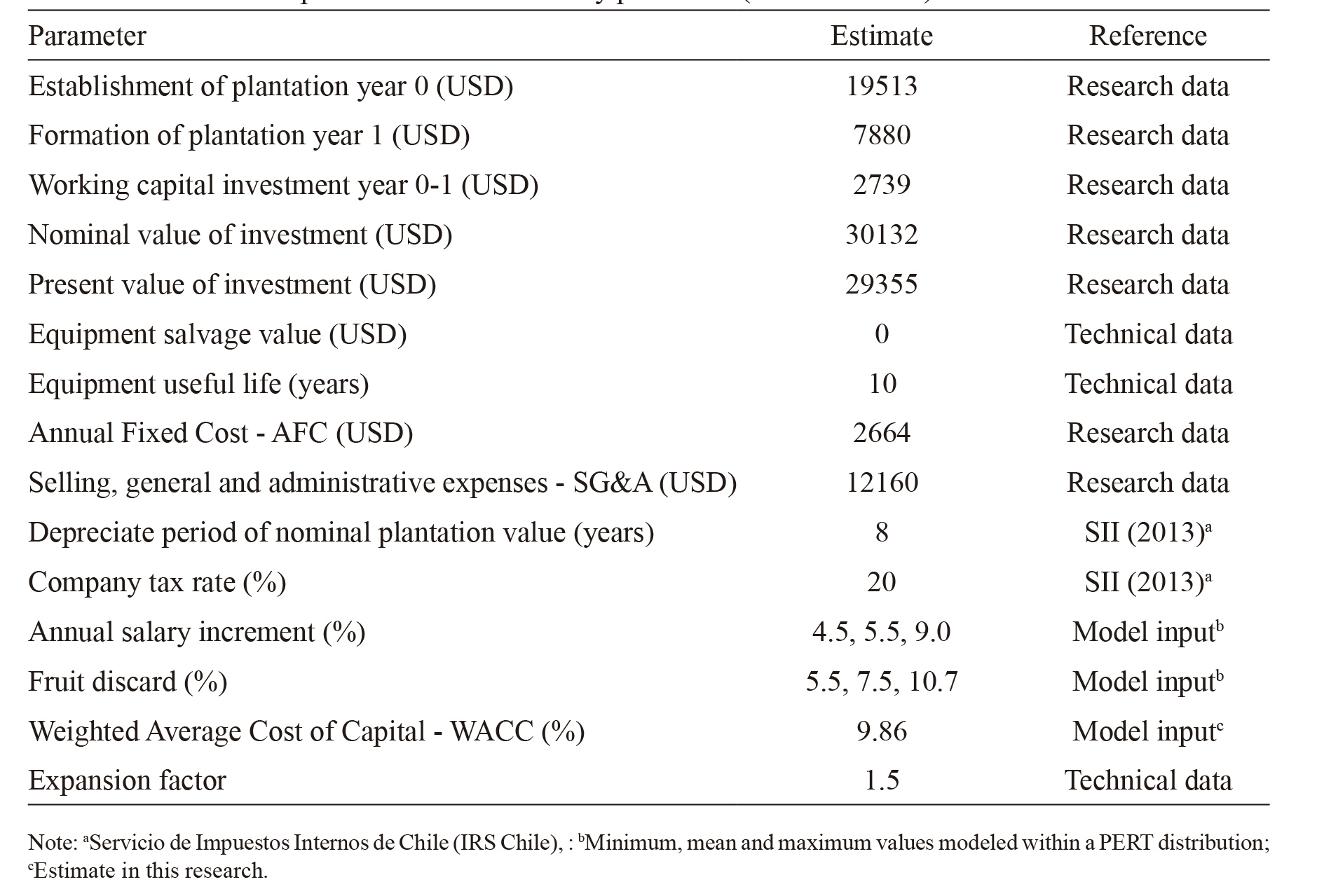
The technical-economic coefficients used for the valuation of the investments and costs were taken from the historical records of ten properties located in the province of Linares (35 ° 51’ S and 71 ° 35’ W), Maule Region, Chile. According to statistics Maule Competitiveness Center (MCC 2010), Linares has the highest proportion of blueberries planted in the Maule Region (64%), representing 16.4% of the national surface area. Starting from the historical information an estimate of the profitability for a 10- year evaluation horizon was carried out, considering 15 ha as a unit of analysis, which is regarded as the minimum profitable planting size for this crop.This minimum size was estimated based on the study of HERNÁNDEZ and MUÑOZ, 2006. The distribution of plants was estimated with a distance of 1 m between plants on the row and 3 m between rows which determines a density of 3,333 plants ha^-1(MUÑOZ, 2010). To estimate relevant net cash flows, it was considered that the first year corresponds to the establishment of the crop stage; the second year corresponds to the formation stage and the third year corresponds to the maintenance stage, considering a normal useful life of nine years for the plantation.The unit values used for the investments and costs valuation were estimated from the per unit average values paid during the 2009/10 agricultural season. In the case of labor, social laws, proportional holidays, unemployment insurance, benefits and production bonuses were included; the other per unit values were considered tax-free. All other per unit values were considered at their market price, excluding tax.

Discount rate

The CAPM, or Capital Asset Pricing Model (SHARPE, 1964) was used to calculate WACC,or Weighted Average Cost of Capital (MILES; EZZELL, 1980). The mathematical expression of the CAPM model is: k_s = R_F + (R_M - R_F) b^L_J where k_s is the cost of capital of a company with debt,RF it is the rate of return on a risk-free asset, RM is the return of an efficient portfolio representative of the market and bL J is the beta factor of an j active representative of the type of business that is being evaluated. To obtain RF, the annualized average real return of Banco Central de Chile bonds was used for the 10-year period from January 2008 to December 2012 (60 data items). To obtain RM the General Index of Stock Prices (or IGPA) of the Santiago Stock Exchange was used to get real annual returns for the period 2000 to 2012. As a proxy company, the beta factor of Frutícola VICONTO S.A. (with debt) was considered, which was obtained from Economatica system on the basis of real closure returns, adjusted for dividends of the past 60 months. The values obtained were as follows: RF = 2.79, RM= 13.5 and . Replacing the previous values in the CAPM expression, we obtain ks = 14.25. The assumption of this calculation is that the business we are evaluating keeps the same debt structure of VICONTO S.A. To obtain the WACC, the expression WACC = KS. E/V + Kd . D/Y . (1-T) was used, where E is the estate, V is value, Kd is the cost of debt, D is debt and T is the income tax rate on companies in Chile (T=0.2). As cost of debt, it was considered the annualized interest rates real average of 30 to 365 days placements of the Chilean financial system in the period from January 2008 to December 2012 (Kd = 4.37). The E/V = 0.67 and D/V = 0.33 relations obtained from the VICONTO S.A. balances to December 30, 2012 were studied. Replacing the values obtained in the cost of capital expression, it was finally obtained WACC = 9.86, which agrees with the real annual discount rate used in this study.

Investments and economic feasibility analysis

Using a partial budget approach all predicted revenues and expenses resulting from investing in a blueberry plantation over the ten-year investment period were collected. Revenues were estimated considering the actual marketed blueberries production and the real exchange rate. Annual Total Variable Cost (TVC) included Annual Direct Variable Cost (DVC) and Annual Indirect Variable Cost (IVC). DVC and IVC included Direct Labor Cost (DLC), Packaging Materials Cost (PMC in USD kg^-1), Harvesting Material Cost (HMC in USD kg^-1), Machinery and Equipment Services (MES in USD ha^-1), Farm Input Cost (FIC in USD kg^-1), Irrigation Cost (IRC in USD ha^-1) and Power and Utilities Cost (PUC as electricity, fuel, refrigeration, water and freight costs). FIC included fertilizers, insecticides, fungicides, herbicides and others agrochemical products. Annual Total Fixed Cost (TFC) included Direct Fixed Cost (DFC) and Indirect Fixed Cost (IFC) as labor for analyzing data, maintenance, depreciation, taxes, insurance and water rights.Annual Selling, General and Administrative Expenses (SG&A) included labor for administration and sales, accounting, advisory, communication, fuel and rents. See in equation 11.

(10)Annual cost of production formulas 11.1 DVC + IVC = DLC + PMC + HMC + MES+ FIC + IRC + PUC 11.2 TVC = DVC + IVC 11.3 TFC = DFC + IFC 11.4 SG&A are Selling, General and Administrative Expenses and, 11.5 TCQ = TVC + TFC are Total Cost of Production, Fixed and Variables or Direct and Indirect.

We suppose that farmer owns the land and therefore the cost of the use of the land was included as the alternative cost of renting the land, after taxes. The latter was calculated as the alternative cost of the invested capital in the field, which was valued at its commercial valuation. The calculation was made considering the commercial value of the land, estimated at 8,000 USD ha^-1, multiplied by the WACC relevant to the farmer (see table 2).

Investments were depreciated using straight-line depreciation over an eight-year period. Taxes were calculated using the 20% tax rate. Net cash flows were collected and adjusted by their respective discount rates. Finally, the NPV was calculated by collecting the discounted cash flows.

Profitability and economic efficiency indicators were calculated for producers with land, according to what is suggested by different authors (BEWLEY et al., 2010; XU et al., 2010; HACHICHA et al., 2011): NPV, IRR and VaR. To measure the economic efficiency, the Average Total Cost (ATC), Unit Contribution Margin (UCM) and Return on Equity (ROE) were calculated. For the purposes of the calculation of the ROE, the current value of the plantation, including the stages of establishment and formation of the crop, and the value of the ground considering its commercial pricing, was considered as working capital.

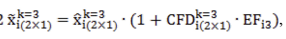
(11) NPV, IRR and ROE stochastic formulas (Eq. 10), (Eq.11), (Eq.12), (Eq.13). 12.1

12.2 NPV = 0 implies that

0 where 0 = IRR 12.3

12.4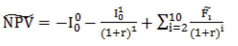

In 12.1 NPV is stochastic NPV, I0 0 is the initial investment in year 0 (or plantation establishment), I10 is the initial investment in year 1 (or plantation formation), F1 is the stochastic net cash inflow in period i and r is the discount rate (or WACC). In 12.3 as PB is stochastic price of blueberry then UCM is stochastic UCM. The ROE formula is a farm’s net income (for purpose of this study it was considered as F1) divided by its Average Stockholder’s Equity (ASE), which were estimated as Present Value of the Plantation (PVP), including the stages of establishment and formation of the crop, and the price of land valued at its commercial appraisal.

Simulation analysis

Following BEWLEY et al. (2010), and recognizing that a deterministic model ignores the uncertainty inherent in a fruit system, a Monte Carlo simulation was conducted using the @Risk addin. In each simulation, Latin Hypercube sampling was used with a fixed seed of 31,759 to ensure all simulations provided repeatable results. The Latin Hypercube sampling method is a technique similar to a Monte Carlo but more efficient (RUBINSTEIN, 1981). To illustrate the importance of capturing the effect of the intra-temporal correlation, the simulation was repeated in two scenarios considering the assumptions of no correlation and only intra-temporal correlation.

RESULTS AND DISCUSSION

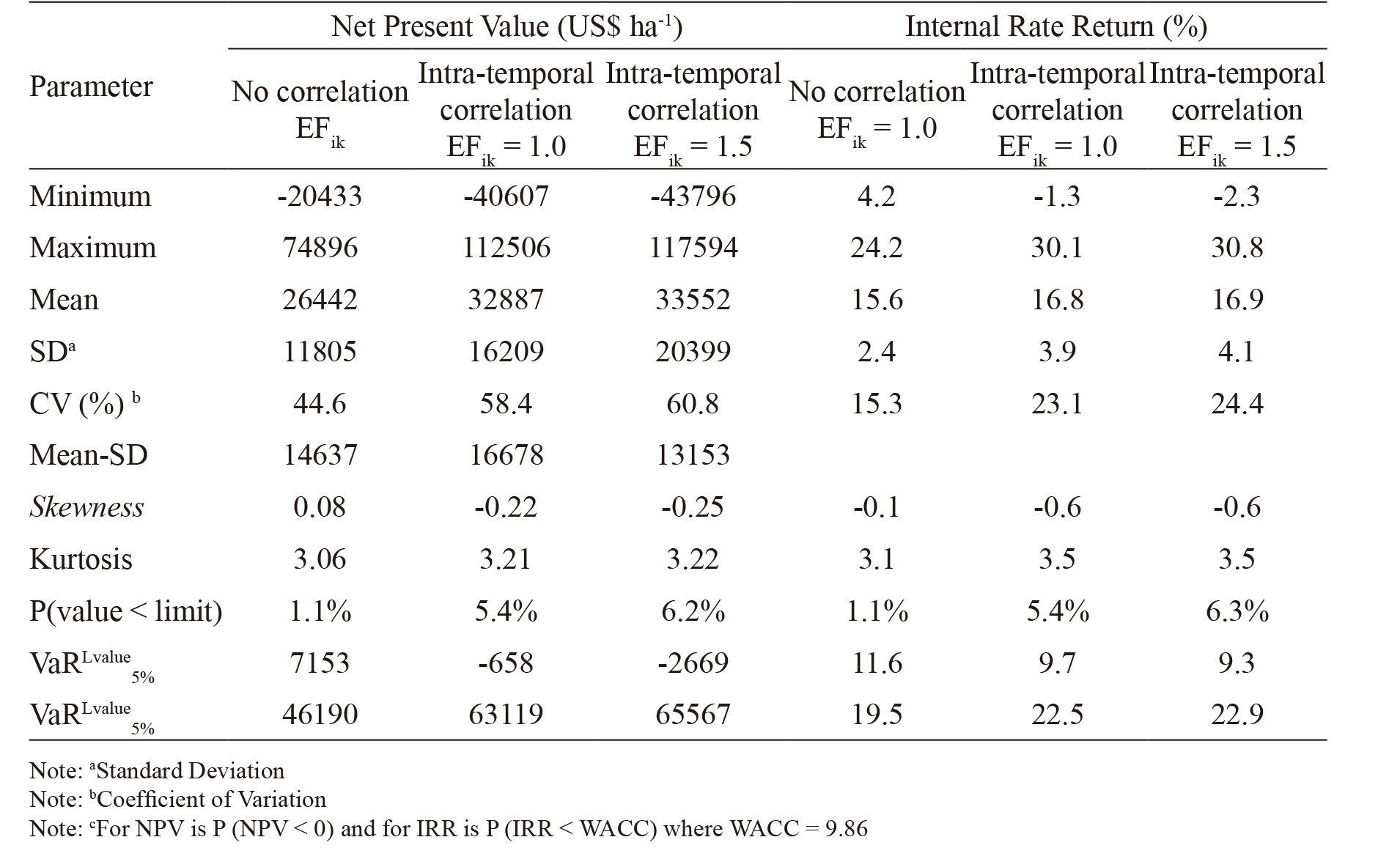
Table 3 presents the main results of the simulations for the assumptions of no correlation and only intra-temporal correlation. When the intra-temporal correlation is included, the minimum NPV value decreases by $ US 20,174 (i.e., 98.8%), the maximum NPV increases by US $ 37.610 (i.e., 50.2%) and the average NPV increases by $ US 6,445 (i.e., 24.4%). As Richardson et al. (2000) suggest, the average NPV is only slightly different as we goes from no correlation to correlation.

However, the minimum and maximums for the NPV distribution increase as more correlation is added to the simulation. The inclusion of intratemporal correlation has a greater impact on the tails than on the average values of the distribution.

Since exposure to risk is more significant in the extreme values of the distribution, the inclusion of intra-temporal correlation allows measuring the value at risk in those areas of the probability distribution where the risk could be underestimated. This is also valid when the expansion factor, which reflects the highest relative risk due to the variability in yields during the evaluation period, is integrated. This result has an important implication from the point of view of the design of agricultural policies. This is because the public managers are usually interested in implementing policies and instruments that contribute to reduce the risk faced by agricultural producers, which requires an adequate characterization of the sources of risk, in this case the yield risk associated with the blueberries production function. In this way, the incorporation of the intra-temporal correlation in the multivariate simulation process allows a better measurement of the joint impact of the performance and the impact of a policy aimed to reduce this type of risk. Therefore, the design of risk management instruments in agriculture should consider not only the intrinsic risk but also the risk associated with intra-temporal correlation between different input variables.

In general, the results show that the plantation project is profitable from the economic point of view, for the no correlation and only intra-temporal correlation assumptions, with positive average values for NPV, in addition to an IRR greater than WACC. However, when the intra-temporal correlation is included, the coefficient of variability (CV) increases, thus reflecting the highest relative risk that the producer truly faces when the intratemporal correlation between random variables is incorporated. In this latter case it is also observed that there is a 5.4% of probability of observing a negative NPV, while this likelihood is only 1.1% in the former case. This probability increases to 6.2% when including the expansion factor. In addition, without including the intra-temporal correlation, the VaR5%Lvalue is greater than zero, while when the intra-temporal correlation and the expansion factor are included, this value is less than zero, gradually increasing the producer’s exposure to risk. Then, the non-inclusion of the intra-temporal correlation would underestimate the risk faced by the agricultural producer, such as suggested by the works of RICHARDSON et al. (2000), EMBRECHTS et al. (2002) and BLUM; DACOROGNA (2004).

This result also has important implications on the decision making of the Chilean farmers, especially if we consider that most of them are averse to risk (TOLEDO; ENGLER, 2008). This could explain why the fruit producers of Chile normally have an inversion portfolio with different types of fruit trees, and therefore with different levels of risk and profitability, implicitly applying the fundamental principle of portfolio diversification, so as to seek the maximum profitability of the business at the lowest possible risk. However, to have more clarity on this, it would require research about the formation of optimal fruit investment portfolios in Chile, which is outside the scope of this study.

The benefit of this project can also be visualized when considering that the difference between NPV and its Standard Deviation (SD) is greater than zero in all considered cases (no correlation and intra-temporal correlation, with EFik = 1,0 and EFik = 1,5) . However, the weakness of this decision rule, defined by MANOTAS & TORO (2009) to determine the suitability of a risky investment, is that it does not consider the confidence level that a decision maker would desire. Different adjustments for the NPV Probability Density Function (PDF) were tested, such us Chi-square (X2), Anderson-Darling (AD) and Kolmogorov- Smirnov (KS) tests. However, the best adjusted is = RiskWeibull function using Anderson-Darling statistic for the NPV as a way to emphasize a greater adjustment in the distribution tails, which precisely reflect the producer exposure to risk (NPV at risk). The Weibull distribution is also one of the few distributions that can be used to model data presenting negative asymmetry, as is the case in this study, where a skewness = - 0.22 was obtained. It is noteworthy that while both the AD test and the KS test give more weight to the tails, X2 give more weight to the central part of the probability distribution.

The average values obtained for the IRR are higher than the discount rate used, which indicates that it is advisable to invest in this type of fruit. This is consistent with the profitability results obtained by different authors for different types of fruit plantations: Lobos and Muñoz (2005) for apples (IRR=12.1%) in Chile, Uzunöz and Akçay (2006) for Pears (IRR=25.1%) and apples (IRR=22.1%) in Turkey, and KREUZ (2002) for apples (IRR between 21.1% and 22.6%) in Brazil. In general, the lower values of the IRR for blueberries in Chile could be explained by the crop yields and selling prices considered because the IRR is highly sensitive to changes in any of these two variables.

The results obtained for IRR1, IRR2,...IRR10000 (because we have 10,000 iterations) are ordered in ascending order so as to obtain the CDF. The distribution function is estimated from the following empirical distribution: Fn(IRR)=(#IRRi=IRR)/n which corresponds to the relative frequency of the IRR, where #IRRi is the number of results of the IRRi obtained from the simulation, which are smaller than a specific value of the IRR. In a similar way to the calculation of the NPV at risk, the IRR at risk can be obtained from its CDF. Therefore, the IRR at risk for the 5th percentile is 9.71% and, in addition, with a 5.4% of probability it is possible to expect an IRR of less than 9.86% (WACC).

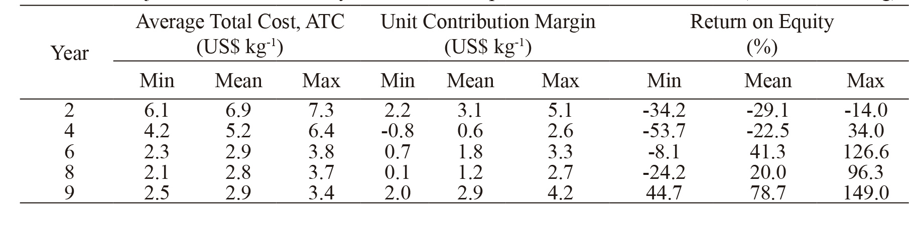
The ATC decreases during the evaluation period, reaching the lowest values between 2.8 and 2.9 US$ kg^-1 for the years of the plantation’s full production, due mainly to the fact that TFC and SG&A are distributed among a larger number of kilos produced. Given that the average price values are higher than ATC, then the UMC mean values are positive. In the case of ROE, the mean values are negative during the first years of growing because the crop yields are not sufficient to generate positive earnings. In general, the results projected for ATC, UMC and ROE are strongly associated with the yield curve of the two species of blueberries considered in this study, reaching full production conditions from year 6. This year also coincides with the time when the capital invested in the project is recovered (Payback).

From the Dupont analysis point of view, the magnitude of the UMC is very relevant, due to the fact that it is probably the main source of profitability in this type of business, understood as the return on investment dimension.

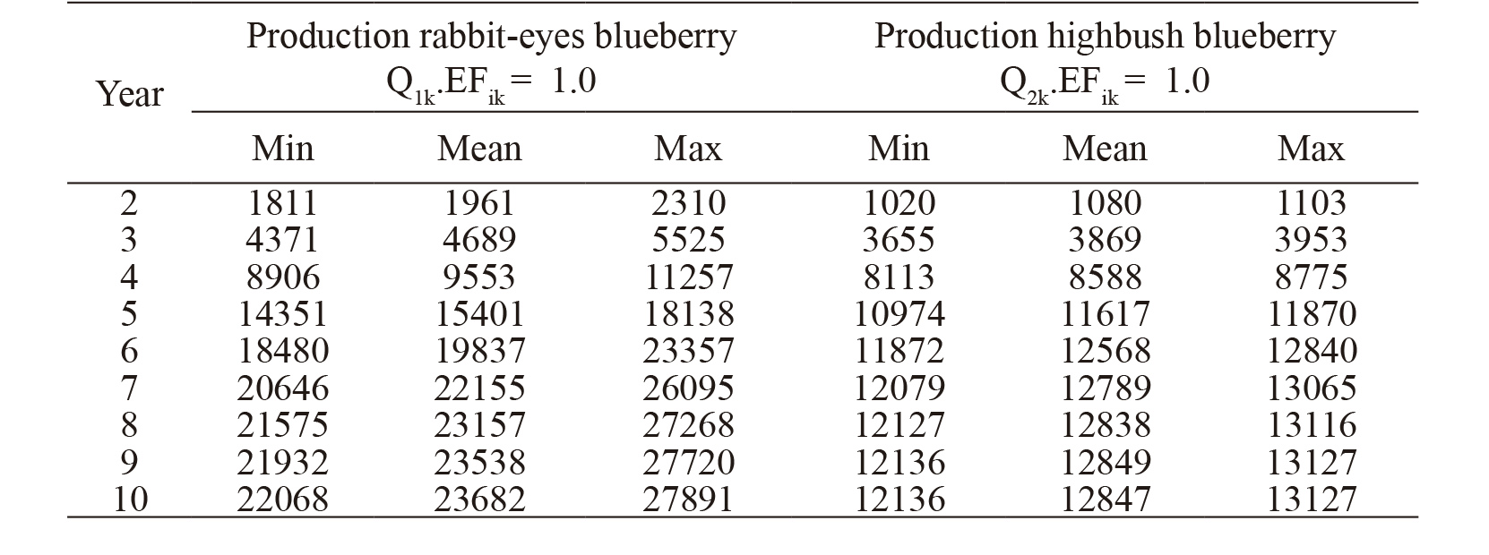
The values simulated for the production evaluation horizon of Q1 and Q₂ are presented intable 5 (expansion factor of 1.0). The parameters of this distribution can be used, for example, to simulate a situation with other risk expansion factor, the effects of a technological change affecting the average yields, the incorporation of a new variety of blueberry, or even a change in the Government’s agricultural policy; all this, without affecting the relative variability between the production variables.

The technique described in this study can easily be applied to other type of fruit tree investments with a nonlinear function of growth. For that it is necessary to have sufficient information about crop age and crop yields in the area of study.

Finally, this project seems to be an interesting investment alternative in fruit trees in Chile, considering that the NPV average values are greater than zero and IRR is greater than the cost of capital, even if the VaR of the project indicates that there exist a probability of obtaining a NPV less than zero.

TABLE 1
Estimates of parameters (b1, b2, b3, b4), square means of the residue (CMR) and coefficient of determination (R2) for the adjusted growth models in rabbit-eye blueberry (QR) and highbush blueberry (QH).

TABLE 2
Investment parameters for a blueberry plantation (values for 1 ha).

TABLE 3
Simulated principal statistics over 10,000 iterations EFik is expansion factor for each year.

TABLE 4
Projected values for some year of simulated period, over 10,000 iterations (values in US$ kg).

TABLE 5
Projected values for each year of simulated period, over 10,000 iterations, 9 years (values in kg ha-1). EFik is expansion factor for each year.

CONCLUSIONS

The traditional method of net present value (NPV) to analyze the economic profitability of an investment (based on deterministic approach) does not adequately represent the implicit risk associated with different but correlated variables. Using a stochastic simulation approach for evaluating the profitability of blueberry production in Chile, the objective of this study is to illustrate the complexity of including risk in economic feasibility analysis when the project is subject to several but correlated risks.

A blueberry investment is subject to various uncertainties. Some sources of uncertainty include variability in production, variability in yield and input and output price variability. The simulation analysis in this study shows that incorporating the intra-temporal correlation between input variables increases the variability of the NPV probability distribution. In fact, since exposure to risk is more significant in the extreme values, the inclusion of intra-temporal correlation increases the probability of a negative NPV.

This result suggests that including intratemporal correlation between inputs variables is critical in economic feasibility analyses. The non-inclusion of this intra-temporal correlation underestimate the risk associated with investment decisions. The same approach used in this study can also be applied in other agricultural sectors.

ACKNOWLEDGEMENT

The authors are grateful for the support received from the Dirección de Investigación of the Universidad de Talca.

• ALI, J.; GUPTA, K. B. Agricultural price volatility and effectiveness of commodity futures markets in India. Indian Journal of Agricultural Economics,Bombay, v.62, p.537-538, 2007.
• BEWLEY, J. M.; BOEHLJE, M. D.; GRAY, A. W.;HOGEVEEN, H.; KENYON, S. J.; EICHER, S.D.; SCHUTZ, M. M. Stochastic simulation using @Risk for dairy business investment decisions.Agricultural Finance Review, Bingley, v. 70, p.97-125, 2010.
• BLUM, P.; DACOROGNA, M. Dynamic financial analysis, understanding risk and value creation in insurance. In: TEUGELS, J.; SUNDT, B. (Ed.).Encyclopedia of actuarial science. New York: John Wiley and Sons, 2004. 15p.
• BOX, G. E. P.; JENKINS, G. M.; REINSEL, G. C.Time series analysis: forecasting and control. New Jersey: John Wiley & Sons, 2007.
• BUGUK, C.; HUDSON, D.; HANSON, T. Price volatility spillover in agricultural markets: an examination of U.S. catfish markets. Journal of Agricultural and Resource Economics, Bozeman,v. 28, p. 86-99, 2003.
• DICKEY, D. A.; FULLER, W. A. Distribution of the estimators for autoregressive time series with a unit root. Journal of the American Statistical Association, New York, v. 74, 427-431, 1979.
• EMBRECHTS, P.; McNEIL, A.; STRAUMANN.D. Correlation and dependence in risk management:properties and pitfalls. In: DEMPSTER, M. A. H. (Ed.). Risk management: value at risk and beyond.Cambridge: Cambridge University Press, 2002. 47p.
• GOMPERTZ, B. On the nature of the function expressive of the law of human mortality, and on a new mode of determining the value of life contingencies. Philosophical Transactions of the Royal Society of London, London, v. 115, p. 513-583, 1825.
• HACHICHA, S.; KAANICHE, L.; ABID. F. Sequential investment and delay: an agribusiness firm case study. Agricultural Finance Review, Bingley,v. 71, p. 240-258, 2011.
• HERNÁNDEZ, C.; MUÑOZ, R. Compañía productora y comercializadora de arándanos frescos UTALCA: Plan de negocios MBA, 2006.14p.
• HOWLEY, P.; DILLON, E. Modelling the effect of farming attitudes on farm credit use: a case study from Ireland. Agricultural Finance Review,Bingley, v. 72, p. 456-470, 2012.
• KHAN, S.; RENNIE, M.; CHARLEBOIS. S. Weather risk management by Saskatchewan agriculture producers. Agricultural Finance Review, Bingley,v.73, p.161-178, 2013.
• KREUZ, C. L. 2002. Investment return for Gala apple cultivar using two planting densities. Pesquisa Agropecuária Brasileira, Brasília, v. 37, p. 229-235, 2002.
• LAW, A. M.; KELTON, W. D. Simulation modeling and analysis. New York: McGraw-Hill, 1991.
• LOBOS, G.; MUÑOZ, T. Índices de estacionalidad de los precios medios recibidos por los productores de manzanas chilenas. Pesquisa Agropecuária Brasileira, Brasilia, v.40, p.1051-1057, 2005
• MANOTAS, D. F.; TORO, H. H. Análisis de decisiones de inversión utilizando el criterio valor presente neto en riesgo (VPN en riesgo). Revista Facultad de Ingeniería, Arica, v. 49, p. 199-213,2009.
• MCC - Maule Competitiveness Center. 2010.Disponivel em: http://www.ccmaule.cl/wp-content/uploads/2014/02/Cluster-Arandanos.pdf. Acesso em: 24 abr. 2015.
  » http://www.ccmaule.cl/wp-content/uploads/2014/02/Cluster-Arandanos.pd
• MUÑOZ, C. Cultivo del arándano en Chile. In: SIMPÓSIO NACIONAL DO MORANGO, 5.,ENCONTRO SOBRE PEQUENAS FRUTAS E FRUTAS NATIVAS DO MERCOSUL, 4., 2010,Pelotas. Proceedings… p.52-58.
• PHILLIPS, P. C. B.; PERRON, P. Testing for a unit root in time series regressions. Biometrika,Cambridge, v. 75, p. 335-346, 1988.
• RICHARDS, F. J. A flexible growth functions for empirical use. Journal of Experimental Botany,Lancaster, v. 10, p. 290-300, 1959.
• RICHARDSON, J. W.; HERBST, B. K.; OUTLAW,J. L.; CHOPE-GILL II, R. Including risk in economic feasibility analyses: the case of ethanol production in Texas. Journal of Agribusiness, Athens, v. 25,p. 115-132, 2007.
• RICHARDSON, J. W.; KLOSE, S. L.; GRAY,A. W. An applied procedure for estimating and simulating multivariate empirical (MVE) probability distributions in farm-level risk assessment and policy analysis. Journal of Agricultural and Applied Economics, Lexington, v. 32, p. 299-315, 2000.
• RUBINSTEIN, R. Y. 1981. Simulation and the Monte Carlo method. New York: John Willey & Sons, 1981.
• SEKHAR, C. S. C. Agricultural price volatility in international and Indian markets. Economic and Political Weekly, Bombay, v. 39, p. 4729-4736,2004.
• SHARPE, W. F. Capital asset prices: a theory of market equilibrium under conditions of risk. Journal of Finance, New York, v. 19, p. 425-442, 1964.
• TOLEDO, R.; ENGLER, A. Risk preferences estimation for small raspberry producers in the Bío-Bío Region, Chile. Chilean Journal of Agricultural Research, Santiago de Chile, v. 68, p. 175-182, 2008.
• UZUNÖZ, M.; AKÇAY, Y. A profitability analysis of investment of peach and apple growing in Turkey.Journal of Agriculture and Rural Development,Mbabane, v. 107, p. 11-18, 2006.
• VERHULST, P. F. Notice sur la loique la population poursuitdans son accroissement. Correspondance Mathématique et Physique, Bruxelas, v. 10, p.113-121, 1838.
• VON BERTALANFFY, L. Quantitative laws in metabolism and growth. Quarterly Review of Biology, Baltimore, v. 32, p. 217-231, 1957.
• WEIBULL, W. A statistical distribution function of wide applicability. Journal of Applied Mechanics,New York, v. 18, p. 293-297, 1951.
• WILLIAM, W. W.; DAHL, B. L. Grain contracting strategies to induce delivery and performance in volatile markets. Journal of Agricultural and Applied Economics, Lexington, v. 41, p. 363-376,2009.
• XU, W.; FILLER, G.; ODENING, M.; OKHRIN. O.On the systemic nature of weather risk. Agricultural Finance Review, Binglev, v. 70, p. 267-284, 2010.

Publication Dates

• Publication in this collection
  Oct-Dec 2015

History

• Received
  18 July 2014
• Accepted
  20 May 2015