VARIETIES OF DIFFERENCE-MAKERS: CONSIDERATIONS ON CHIRIMUUTA’S APPROACH TO NON-CAUSAL EXPLANATION IN NEUROSCIENCE

Abstract

Causal approaches to explanation often assume that a model explains by describing features that make a difference regarding the phenomenon. Chirimuuta claims that this idea can be also used to understand non-causal explanation in computational neuroscience. She argues that mathematical principles that figure in efficient coding explanations are non-causal difference-makers. Although these principles cannot be causally altered, efficient coding models can be used to show how would the phenomenon change if the principles were modified in counterpossible situations. The problem is that efficient coding models also involve difference-makers that, prima facie, cannot be characterized as non-causal in this sense. Mathematical principles always involve variables which have counterfactual (instead of counterpossible) relations between them. However, we cannot simply assume that these difference-makers are causal. They can also be found in paradigmatic non-causal explanations and therefore they must be characterized as non-causal in some sense. I argue that, despite appearances, Chirimuuta's view can be applied to these cases. The mentioned counterfactual relations presuppose the counterpossible conditionals that describe the modification of a relevant mathematical principle. If these conditionals are the hallmark of non-causal relations, then Chirimuuta’s criterion has the desired implication that variables in mathematical principles are non-causal difference-makers.

Keywords:
Computational neuroscience; Non-causal explanation; Difference-makers

1. INTRODUCTION

The mechanistic approach to explanation or ‘new-mechanism’ (hereafter, ‘mechanism’) is currently a dominant perspective in the philosophy of neuroscience. Part of this success can be attributed to the fact it provides a unified framework to account for the explanatory power of very diverse models that can be found within the field. It has proven to be useful to characterize models ranging from molecular to behavioral neuroscience¹. However, there are good reasons to believe that it cannot be employed to understand relevant abstract models. According to some authors, mechanism implies that abstract models are not fully explanatory. For example, Chirimuuta (2014) claims that mechanism is committed to a requirement she calls “the More Details the Better” (MDB). MDB implies that models which omit some information about the target mechanism (e.g. models that describe only “high level” properties), are less explanatory than more detailed descriptions. In response to interpretations of this sort, mechanistic criteria for building abstract models have been proposed (e.g. Levy & Bechtel 2013, Boone & Piccinini 2016). The problem is that although mechanism is compatible with some abstractions, there are features that cannot be omitted from a model without making it non-mechanistic. Mechanistic explanation requires some information about the causal properties or relations of its target system (Levy and Bechtel 2013).

Batterman (2010), Rice (2012, 2015) and Batterman & Rice (2014) have argued that some minimal models in physics and biology (that is, models which abstract away from many details of a system in order to highlight dominant and general features) are non-causal. The presence of non-causal models in cognitive neuroscience would imply that mechanism cannot provide a general account and therefore, we should endorse some form of pluralism about neurocognitive explanation. Chirimuuta (2017) claims that efficient coding models in computational neuroscience are a non-causal variety of minimal model. Furthermore, Chirimuuta undermines the strategy of saying that these models are non-explanatory by showing that they satisfy a criterion for explanatory relevance accepted by many mechanists. Efficient coding models are able to answer relevant what-if-things-had-been-different questions, or “w-questions”, regarding their explananda. These are questions about how the explanandum would change in the counter-factual situation in which the explanans is different in some specific way. An explanatory model implies counterfactual conditionals that answer such w-questions.

The ability of a model to address these w-questions is supposed to account for its explanatory power because it implies that the model describes features that are ‘difference-makers’ for its explanandum. Usually, these difference-makers are causal in the sense that the counterfactual situation to which a w-question refers results from an intervention on a relevant aspect of the explanans. However, Chirimuuta points out that some w-questions refer to scenarios that are mathematically different from the actual world and therefore cannot result from an intervention (that is, they refer to counterpossible situations). The answers to these w-questions are counterpossible conditionals which involve non-causal difference-makers. These define a non-causal explanation. Chirimuuta claims that efficient coding explanations are non-causal in this sense.

Chirimuuta’s proposal widens the scope of neurocognitive explanatory models (by including non-causal models) and, at the same time, vindicates the mechanistic idea that explaining is a matter of identifying difference-makers. This means that, if we abandon the requirement that explanation must be causal, we can use part of a mechanistic framework to provide a unified characterization of explanation in cognitive neuroscience. In this respect, her proposal is similar to the one advanced by Jansson & Saatsi (2017). They also argue that the explanatory power of both causal and non-causal models can be accounted for by the difference-makers they describe. Chirimuuta’s distinctive insight is that non-causal models describe a special kind of difference-maker. This idea conciliates pluralist and monist intuitions about explanation in neuroscience. Her approach contributes both to understanding what is common to different neurocognitive explanations and to characterizing the differences between them. Nevertheless, I will argue that this proposal has a significant shortcoming.

The explanatory power of efficient coding models depends on difference-makers that, prima facie, cannot be characterized as non-causal in Chirimuuta’s sense. Mathematical principles always involve variables which have counterfactual (instead of counterpossible) relations between them. However, we cannot simply assume that these difference-makers are causal because they can also be found in paradigmatic cases of distinctively mathematical explanations described by Pincock (2007) and Lange (2013). They must be characterized as non-causal in some sense. The goal of this paper is not merely to point out this problem but also to suggest a possible solution. I propose to characterize the problematic difference-makers by combining Chirimuuta’s approach with some neglected aspects of Woodward’s proposal.

His interventionist view implies that the difference-making relation between the variables of a system always presupposes an ‘invariance’. This is simply the generalization in which these variables figure, which remains unchanged in the counterfactual situations required to characterize the mentioned relation. I will argue that if we follow Chirimuuta’s idea that not only variables but also invariances must be understood as difference-makers, then an explanation involves two kinds of conditionals which are closely related. Specifically, I will claim that the counterfactual conditionals that describe the relation between the variables of a system presuppose (either counterfactual or counterpossible) conditionals that describe the modification or ‘modulation’ of the relevant generalization. This implies that when the generalization is a necessary mathematical principle, the characterization of the difference-making relation between its variables presupposes counterpossible conditionals. If these conditionals are the hallmark of non-causal relations, then Chirimuuta’s criterion now has the implication that variables in mathematical principles are non-causal difference-makers.

The paper is structured as follows. In section 2, I describe two efficient coding models: Sarpeshkar (1998) hybrid neural computation model and Laughlin & Attwell (2001) sparse neural coding model. I present Chirimuuta’s proposal and claim that these models refer to difference-makers which apparently cannot be characterized as non-causal in her sense. In section 3.1, I show why these difference-makers are problematic and I argue that an adequate approach to non-causal explanation must characterize them as non-causal. Finally, in section 3.2 I suggest how we can apply Chirimuuta’s criterion to these cases.

2. EFFICIENT CODING EXPLANATIONS AND TWO KINDS OF W-QUESTIONS

Efficient coding models provide computational or information-theoretic explanations of why neurons, neural circuits or neural systems behave in the ways they do. Chirimuuta (2014) pointed out that they are similar to optimality models in biology. Based on this idea, I will characterize efficient coding explanations by borrowing some concepts from the optimality framework (see Rice 2015)².

An efficient coding model explains the efficiency of a given brain structure in the performance of a given task by considering different computational or informational strategies for that task. In the first place, the model describes a set of alternative computational and/or information-theoretic strategies for the relevant task. For instance, Atwell and Laughlin (2001) present a set of alternative coding regimes that a neural population could employ for representing a given number of conditions. In the second place, the model shows that one of these strategies is the most efficient by determining that, given certain constraints, it optimizes some ‘design variables’. These variables represent parameters of information transmission which are relevant for the task. The model also specifies an optimization criterion for each design variable, that is, it determines whether it needs to be minimized or maximized. That a given strategy optimizes a given set of design variables only means these would have less optimal values (lower or higher, depending on the optimization criterion) if an alternative strategy was implemented. For instance, Attwell and Laughlin (2001) show that sparse coding is an optimal strategy because given a specific number of conditions that a system needs to represent (a constraint imposed by the information processing task), it minimizes (optimization criterion) energy consumption (the design variable) better than local coding (the relevant alternative strategy). In the third place, we must assess whether the optimal strategy and the one actually employed by the target neural structure line up. If there are enough similarities, we have an explanation of how the relevant brain structure manages to optimize the design variables that characterize the relevant task.

It is important to point out that there can be some significant variations within this general framework. For instance, as we will see briefly, in some models the different strategies are not correlated with different values of design variables but rather with equations that relate these variables in different ways. Also, sometimes design variables are in conflict with each other. In this case, we say that there is a trade-off between them. But this is not necessarily so. Some models refer to a single design variable whose optimization is only limited by the available strategies and environmental constrains. What I take to be the essential feature of efficient coding models is defining a strategy set and showing how each strategy in that set modifies the behavior of design variables (their values or relation to each other) in a way that is relevant to their optimization. This is all that is required to show that a given computational or informational strategy is the most efficient for a given task.

2.1 Hybrid computation

Chirimuuta presents an efficient coding model proposed by Sarpeshkar (1998) to explain neural computation. To this end, neural computation is compared with other known computational systems (i.e., with alternative computational strategies). Sarpeshkar examines how digital and analog computational systems differ regarding resources consumption and precision. The main idea is that digital systems are much more expensive than analog systems to process the same amount of information but are also more precise, that is, they have a higher signal to noise ratio. Analog and digital systems fail to optimize resource consumption and precision at the same time. Sarpeshkar shows that hybrid computation, the strategy that is likely implemented by the brain, can optimize both parameters.

A component of an analog system can represent many bits of information at a given time. This is because it produces signals that vary continuously. Any number of conditions can be represented by different physical states of this signal. In contrast, digital signals can only represent 1 bit of information at any given time because they are all-or-nothing events. This means that a digital system would need as many components as bits of information it needs to transmit, whereas those bits could be transmitted by a single wire in an analogic system.

Despite this advantage, analog systems have the problem that their signals are much more susceptible of being corrupted by noise than digital systems. The more one increases the amount of information that one wants to transmit by employing a single wire the noisier will be the signal. This is because in order to increase its informational capacity (i.e., represent more conditions with a single wire) the difference between the physical magnitudes that codify different signals must decrease. To maintain or increase precision in an analog system one needs to represent the same information by employing more components. However, this will also increase the resources required by the system.

Sarpeshkar offers a mathematical explanation of the fact that the growth in resources consumption required to obtain high precision in analog computation is significant enough to undermine its efficiency. This will constitute the main part of the mathematical framework of his efficient coding explanation. Different strategies are represented by different kinds of components (digital, analog or hybrid). Sarpeshkar estimates power consumption, area consumption and precision (the design variables) for each kind of system by considering the different (information-theoretic) properties of the components that they employ. The optimization criterion for these variables is minimizing area and energy consumption and maximizing reliability or precision.

In this model, strategies (i.e., component types) are not correlated with specific values of design variables but rather with equations that relate these variables in different ways. Each component type is related to a pair of equations, which Sarpeshkar calls “resource/precision equations.” One of the equations represents the trade-off between space consumption and precision and the other represents the trade-off between power consumption and precision. The optimal strategy is the one whose associated equations enable a system to reach the optimal values, that is, the maximum precision at lowest power and area cost. For brevity´s sake, I will just consider the trade-off between power consumption and precision (signal to noise ratio).

The equations that define this trade-off³ determine a power/precision curve for each kind of system (Figure 1).

Figure 1
From Sarpeshkar (1998), the graph represents the behavior of power/precision equations for analog and digital computation.

The graph in Figure 1 shows that precision in digital systems can be enhanced without significant power growth. However, the power baseline for digital systems is too high. On the other hand, analog systems have a low baseline of power consumption but increasing precision very quickly rises power levels above digital computation. Hybrid computation would be the solution to this trade-off between precision and resource consumption. Hybrid components are constituted by analog/digital converters which make possible to alternate between phases of analog and digital processing. Sarpeshkar does not offer, as one would expect, a power/precision equation for hybrid computation to show that it can achieve high precision values at low power values. However, this follows from the fact that hybrid links (the components of hybrid computation) can enhance the precision of analog processing stages without adding new analog components (that is, without significantly increasing power and area consumption) but rather by adding small steps of digital processing within each component.

Sarpeshkar explains the efficiency of neural information processing by arguing that it is likely that the brain implements this optimal computational strategy:

“Action potentials are all-or-none discrete events that usually occur at or near the soma or axon hillock. In contrast, dendritic processing usually involves graded synaptic computation and graded nonlinear spatiotemporal processing. The inputs to the dendrites are caused by discrete events. Thus, in neuronal information processing, there is a constant alternation between spiking and non-spiking representations of information. This alternation is reminiscent of the constant alternation between discrete and continuous representations of information. Thus, it is tempting to view a single neuron as a D/A/D” (Sarpeshkar, 1998, 1630).

Now we can move to the discussion about how this model explains. As mentioned above, causal approaches often maintain that a model explains only if it can be used to determine how the explanandum changes in the counterfactual situation in which the explanans is different in some specific way (e.g., Woodward 2003, Kaplan 2011, Kaplan and Craver 2011, Levy and Bechtel 2013). That is, the explanatory power of a model is determined by its ability to address w-questions. This implies that an explanatory model describes features that are ‘difference-makers’ for its explanandum. Usually, the relation between a difference-maker and a phenomenon is considered causal because the counterfactual situation to which the relevant w-question refers results from an intervention on some aspect of the explanans. An intervention is “an idealized, unconfounded experimental manipulation of one variable which causally affects a second variable only via the causal path running between these two variables” (Woodward 2013, p. 46).

However, Chirimuuta (2017) claims that Woodward’s approach can be generalized beyond causal explanation. Elaborating on a suggestion advanced by Woodward (2003, p. 221), she affirms that properties which cannot be causally modified (i.e., which cannot be affected by an intervention) can make a difference regarding a phenomenon. One of the examples mentioned by Woodward is the hypothesis that the stability of the planets’ orbits depends mathematically on the four-dimensional structure of space-time. Such orbits are stable in a four-dimensional space-time but would be unstable in a five-dimensional space-time. There seems to be no possible (idealized or otherwise) intervention that could result in the modification of the structure of space-time. The question about this counterfactual situation is a non-causal w-question which refers to a non-causal difference-maker. Another example of a non-causal difference-maker is how the truth of some mathematical theorem counterfactually depends on the assumptions from which the theorem is proved (Woodward 2003, p. 220). The mathematical properties or facts to which these assumptions refer constitute non-causal difference-makers regarding the properties or facts to which the theorem refers. A purely non-causal model explains by describing only this kind of difference- maker.

Although these examples provide a rough idea of what a non-causal difference-maker (and a non-causal w-question) is, a more explicit characterization can be provided. In Woodward’s view, the class of counterfactual situations that can be the result of an intervention is quite wide. He affirms that these counterfactuals do not need to be nomologically or physically possible but rather only logically possible. The only situations that cannot be the result of an intervention are those that are inconsistent or incoherent. (Woodward 2013, pp. 132, 133; 2016). This means that, according to this approach, even contingent laws which are modally robust (such as basic laws of physics) can count as causal difference-makers. In turn, purely mathematical principles can be considered non-causal difference-makers. These principles are necessary, which means that alternative principles (i.e., principles that result from modifying in some way the actual ones) are not true in any possible world. We know that these alternative principles are impossible because they involve some kind of inconsistency or contradiction. Mathematical principles cannot be modified by interventions because the relevant modifications only occur in counter-possible situations.

Chirimuuta applies this notion of a non-causal difference-maker to Sarpeshkar’s proposal. As we saw, Sarpeshkar explains the implementation of hybrid computation by describing its relation to the trade-off between resource consumption and reliability. This trade-off is a crucial part of the explanans of hybrid computation and, as such, it is also its difference-maker. The resource/precision equations that describe this trade-off imply that hybrid computation can achieve optimal values for resource consumption and reliability (in comparison to those achievable by analog and digital systems). This relation between the trade-off and hybrid computation can be used to address a relevant w-question about the explanandum (i.e., hybrid neural computation): If this trade-off did not occur then hybrid computation would not achieve these optimal values and therefore there would be no reason to implement this strategy, that is, the brain could have been a purely analog or a purely digital system. Chirimuuta claims that this scenario cannot be interpreted as the result of an intervention because the existence of the trade-off is not an empirical fact about the properties of actual objects but the result of our information-theoretic definitions of digital and analog coding. Given any physical system and given a fixed quantity of information that it needs to transmit, resource investment has a trade-off with the susceptibility of the signal to be corrupted by noise. The information-theoretic explanation of the efficiency of the brain informs us, according to Chirimuuta, about counterfactual scenarios in which the laws of information theory are different. Tinkering with information theory and determining its implications for coding systems cannot be understood as a causal intervention. Therefore, Chirimuuta concludes, efficient coding explanations describe non-causal difference-makers.

I agree with Chirimuuta that the ability to address w-questions about the trade-off is relevant for understanding why Sarpeshkar’s model is explanatory. However, this is not sufficient to show that it provides a purely non-causal explanation. The model is also required to address a different kind of w-questions. We saw that it explains the efficiency of neural information processing by showing that it implements the optimal strategy. I also mentioned that being optimal only means that the actual strategy makes the values of design variables closer to the optimal than any relevant alternative strategy. Therefore, determining a crucial aspect of the explanans (i.e., that the actual strategy is optimal) requires showing what values the design variables can acquire in the counterfactual situations in which alternative strategies are employed by the brain.

These w-questions about alternative strategies do not involve non-causal difference-makers in Chirimuuta’s sense. They do not refer to situations in which the relevant mathematical principles are different from the actual ones. On the contrary, what determines how design variables respond to an alternative strategy are the actual mathematical equations. An alternative computational strategy would generate less than optimal values in counterfactual situations in which the actual resource/precision equations for that strategy are true. The existence of less than optimal computational systems and their corresponding resource/precision equations is not a mathematical impossibility. Human-made digital computers constitute a common instance of these non-optimal information processing systems.

In section 3, will argue that the ability to address these w-questions does not make an explanation causal. But before getting to this point, I would like to show that these questions can also be addressed by an efficient coding model that has a very different mathematical structure. This will support the idea that this is a general feature of efficient coding models. I will consider a model proposed by Attwell and Laughlin to explain the widespread implementation of distributed or sparse neural coding.

2.2 Sparse coding

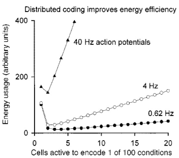
Attwell and Laughlin (2001) explain the efficiency of neural information processing by developing some ideas from Levy and Baxter (1996), constraining them through a detailed energy budget for brain signaling. In order to determine the impact of different coding strategies on neural energy consumption, the authors consider a system that must represent 100 different sensory or motor conditions. A purely local coding strategy is to represent each of the 100 conditions by 1 different active cell to denote each condition (i.e., using 100 neurons to represent 100 conditions). Attwell and Laughlin estimate the energy expenditure of this coding regime by taking R to be the ATP (adenosine triphosphate, the molecule that carries the energy needed for neural signaling) usage per cell on the resting potential, and A the extra ATP usage per cell on active signaling (action potentials and glutamate-mediated signaling). This implies that the total ATP used by the system to signal 1 of 100 conditions under this local coding regime would be 100R + A. As soon as we begin to depart from this local coding regime towards a sparse one, an increase in energy efficiency is patent. If a condition is represented by the simultaneous firing of 2 cells (at the same rate, with the others not firing), only 15 neurons are needed to represent 100 conditions. This is given by the equation (which I will call the “capacity/code/components equation” or “3C equation”) that relates representational capacity or number of conditions represented (R) with the number of cells or components of the system (n) and number of cells active to represent a condition (np):

$R:n!/\left[\left(n-np\right)!\left(np\right)!\right]$

In our case, 3C implies that 15!/(13! 2!) = 105. When we use this code, the energy expenditure is 15R + 2A. If R and A are equal (the energy budget proposed by the authors suggests this is the case for neurons firing at 0.62 Hz), then this distributed representation gives a 6-fold reduction in energy usage for transmitting the same information. Similarly, if a condition is represented by 3 cells firing, 3C implies that only 10 cells are needed to represent 100 conditions (given that 10!/(7! 3!) = 120), and the energy expenditure is 10R + 3A, which (for R=A) is a further improvement of energy efficiency.

In this model, the different values of the variable np (the number of active cells encoding a condition) constitute different coding strategies. The number of conditions represented is a constraint determined by the relevant informational task. The amount of ATP invested in the representation of a condition at a given time is the design variable to be optimized. The model shows which is the optimal strategy by relating the strategies with the design variable. Attwell and Laughlin affirm that the energy used to encode a condition (R + A) is a function of n + np. As we saw, the 3C equation shows how these variables can be modified by switching the coding strategy. Sparse coding is efficient because it can produce a significant reduction of n (in comparison with local coding) by minimally increasing np.

We can now apply Chirimuuta’s criterion to characterize Attwell and Laughlin’s proposal. Although their assessment of the efficiency of sparse coding depends on empirical measurements of neural energy consumption (e.g. ATP consumption by a cell firing at a given rate and at resting potential) their reasoning is based on the mathematical fact implied by the 3C equation, namely, that the number of components required for encoding a given number of conditions dramatically decreases if we use more than one active component to encode each of those conditions. Energy consumption (the design variable) depends on the number of components of the system, which in turn depends on the coding regime in the way specified by 3C. We can say that if 3C were false, then local codes could be optimal for systems that, for example, encode 100 conditions. Given that 3C is a mathematical fact, if Attwell and Laughlin`s model implies this conditional then it also addresses w-questions that refer to non-causal difference-makers.

However, this model must also address the other kind of w-questions (i.e., the ones about alternative strategies). Attwell and Laughlin’s model determines which specific values the design variable (energy usage) has in the counterfactual situations in which an alternative strategy (a different coding regime) is employed. This is precisely what Figure 2 below shows. The graph shows that energy usage under sparse coding is lower than in the counterfactual situation in which local coding is implemented. The model explains the metabolic efficiency of neural representations by showing the optimality of sparse coding, which in turn is implied by what happens in these counterfactual situations.

Figure 2
From Attwell and Laughlin (2001), the graph represents the relation between coding regime and energy usage for neurons that represent 100 conditions firing at 0,62, 4 and 40 Hz.

These w-questions concerning alternative sub-optimal strategies do not involve non-causal difference-makers in Chirimuuta’s sense because they do not refer to situations in which the relevant mathematical relations are different from the actual ones. On the contrary, only if we presuppose that 3C obtains it follows that in the counterfactual situation in which a neural system employs a local code it will need much more components to represent the same conditions (and therefore energy consumption will rise to less than optimal levels). In order to address these w-questions we need to presuppose that the actual mathematical relations are not altered in the relevant counterfactual situations. In what follows I will assess what implications these w-questions have for the characterization of non-causal explanation.

3. NON-CAUSAL DIFFERENCE-MAKERS AND COUNTERFACTUAL SITUATIONS

In section 3.1 I explain why w-questions about alternative strategies are problematic for characterizing non-causal difference-makers. Although it seems that Chirimuuta’s criterion does not apply to strategies, we cannot affirm that they are causal difference-makers. In section 3.2 I suggest that, despite appearances, Chirimuuta’s proposal can be applied to these problematic cases.

3.1 Mathematical explanation and questions about possible situations

It is not obvious why the fact that efficient coding models address the w-questions mentioned in the previous section is problematic for Chirimuuta’s proposal. She affirms that causal and non-causal explanations are often complementary when they have closely related explanantia. For instance, a non-causal model can describe the optimal character of hybrid computation, whereas an etiological model can describe the selective pressures in the evolution of the brain that determined it to be efficient and reliable. The explanations are complementary because one can predict that the selective demand for efficiency and reliability would be optimally satisfied by hybrid processing. However, she maintains that this relation is not problematic because it is clear that the two explanantia are different and therefore, a purely mathematical or non-causal explanation can be isolated.

Moreover, Chirimuuta (2017) claims that even if the non-causal explanation could not stand alone, we could still isolate a non-causal part of an explanation⁴. Perhaps efficient coding models become explanatory only when they include information about the etiological processes that lead a system to the optimal strategy. Nonetheless, Chirimuuta insists that this would only imply a division of labor within the construction of a model. The causal part of the model is that concerned with etiology and the non-causal part is concerned with optimality or efficient information transmission.

The problem is that, as we saw, the purely efficient coding part of a model (one that does not include any information about etiology) needs to describe difference-makers that, prima facie, cannot be characterized as non-causal. As I mentioned, efficient coding explanation requires determining that the actual strategy is optimal and this can only be done by showing how the design variables would respond to alternative strategies. The set of w-questions about sub-optimal alternative strategies is the question about the optimality of the actual strategy. That is, that a strategy is optimal means that alternative strategies have sub-optimal values. If these w-questions do not refer to non-causal difference-makers then a non-causal part of the explanation cannot be isolated.

However, although strategies cannot be characterized as non-causal according to Chirimuuta’s criterion, they must be non-causal in some other sense. This is simply because very similar difference-makers described by Jansson & Saatsi (2017) can be found in paradigmatic cases of non-causal models. They argue that typical mathematical models explain in the same way as causal models do. They discuss proposals (such as the ones advanced by Lange 2013 and Pincock 2007) according to which mathematical models provide sui generis explanations. Their strategy is similar to Chirimuuta’s. They argue that Woodward’s proposal can be extended to mathematical explanation. They claim that the explanatory power of these models is determined by the fact that they describe difference-makers. However, the difference-makers they consider do not involve mathematically impossible situations. This is not a problem for them because they are not concerned with what makes an explanation non-causal but rather with what makes abstract models explanatory. This is why they do not offer a criterion to distinguish between causal and non-causal difference-makers. However, we do need this criterion if we accept that the mathematical difference-makers they describe play an explanatory role and that mathematical explanation is non-causal.

A simple example of a mathematical explanation (provided by Lange 2013) is the explanation of why a mother fails to distribute her strawberries evenly among her children without cutting any. This fact can be mathematically explained by the facts that she has three children and twenty-three strawberries, and that twenty-three cannot be divided evenly by three. Of course, in a genuine mathematical explanation this last fact depends in turn on more general mathematical principles. Here the relevant principles are that (1) b is a multiple of a if b = na for some integer n, that (2) when a and b are both integers, and b is a multiple of a, then a is divisor of b and (3) and a is a divisor of b only if dividing b by a leaves no remainder. These principles explain the failure of the mother in the actual situation because there is no integer that could be multiplied by 3 to obtain 23. Lange claims that an explanation of this kind is non-causal because the relevant mathematical principles have a stronger modal force than any physical law. That is, they are true even in worlds where all the physical laws are not. When a phenomenon is explained only by this kind of principles we have a purely mathematical explanation.

Chirimuuta (2017) claims that her proposal is a way to understand Lange’s idea in terms of difference-makers. For instance, the explanation I mentioned above would answer the question of what would happen if the relevant mathematical principles were false. If this were the case, twenty-three could be evenly divisible by three and the mother could distribute her strawberries evenly among her children without cutting any. This w-question refers to worlds which are farther from the actual one than those mentioned by causal w-questions. This is consistent with Lange’s idea that the modal strength of mathematical principles is relevant to understanding how non-causal models explain.

Jansson and Saatsi (2017) agree that mathematical models refer to principles that are modally stronger than physical laws, but they consider that this does not determine their explanatory power. They claim that mathematical models explain by addressing w-questions that, like the ones I mentioned in the previous section, do not refer to counterpossible situations. For instance, the mentioned explanation answers the question of what would happen if the mother had twenty-one strawberries. This alternative fact and the mentioned mathematical principles imply that the mother would be able to distribute the strawberries evenly among her children without cutting any. This is because there is an integer 7 that can be multiplied by 3 to obtain 21 and 3 and 21 are integers. From this it follows that 3 is a divisor of 21 and therefore dividing 21 by 3 leaves no reminder. This w-question shows that the number of strawberries is a difference-maker for the fact that the mother cannot distribute them evenly among her children. Jansson & Saatsi (2017) claim that difference-makers of this kind account for the explanatory power of mathematical models.

The same idea can be applied to other of the examples discussed by Lange (2013) and introduced by Pincock (2007). The explanation of the fact that no one has ever managed to cross all of the bridges in the city of Königsberg just once, without ever doubling back over a bridge, depends on the characterization of the set of bridges as a network of nodes and edges in graph theory. Here the relevant mathematical principle is that a necessary and sufficient condition for a Eulerian path (that is, the kind of path which allows one to pass through each node only once) is that the graph is connected (that is, there is a path between every pair of vertices) and that is has exactly zero or two nodes of odd degree (where the degree of a node is the number of edges incident to it). The impossibility of passing through all bridges by crossing them only once is explained by this principle and the fact that each of the four nodes in the graph that represents the configuration of the bridges is touched by an odd number of edges.

Euler´s principle is modally stronger than any physical principle and therefore provides a non-causal explanation in Lange’s sense. Also, this explanation has the implication that one could cross all the bridges just once if Euler’s principle were false. The explanation answers Chirimuuta’s w-questions about mathematically impossible situations. However, as Jansson and Saatsi (2017) point out, it also can be used to address the question of what would happen in the (mathematically possible) situation in which each of the four nodes was not touched by an odd number of edges. Euler’s principle implies that in this counterfactual situation if would be possible to pass through each bridge only once.

More generally, mathematical explanations always employ principles which include variables that can be modified in alternative but possible situations. Given that these hypothetical modifications affect the explanandum in some way, the actual values of these variables can be considered genuine difference-makers. However, it is clear that these difference-makers do not make these explanations causal. The mentioned examples are paradigmatic cases in which the explanans only describes mathematical relations. This means any adequate criterion must imply that these difference-makers are non-causal. In the next section I will suggest how Chirimuuta’s proposal can be applied to these cases.

3.2 A possible solution: Invariances and modulation

The key to understanding non-causal difference-makers lies in the close relation that variables and principles or generalizations have within Woodward`s proposal. The difference-making relations that constitute an explanation are characterized in terms of variables related by generalizations. An explanandum M is the statement that some variable Y takes the particular value y. In turn, the explanans E is constituted by the statement that some variable X takes a particular value x and also by a generalization G that relates the values of X and Y.

The condition that Woodward proposes for E to be minimally explanatory (besides the fact that x and y must be the actual values of X and Y, respectively) is that it must be the case that G determines what the value of Y is when X takes the value x and G correctly describes the value y' (where y' ≠ y) that Y would acquire if some intervention changes the value of X from x to x' (where x ≠ x') (Woodward 2003, pp. 202 and 203). That is, G must correctly describe the shape of the difference making relation between X and Y.

Woodward mentions that the generalization G that figures in an explanation has some degree of ‘invariance’ (Woodward 2003, ch. 6). Difference-making relations are about variations: they are constituted by the fact that a dependent variable (or set of variables) would change if the independent variable (or set of variables) is modified. However, these variations would not contribute to the control of the target system unless the relations themselves are stable or invariant (p. 253). The generalization G which specifies how the dependent variable is modified by the independent one must remain the same at least for some sub-set of counterfactual situations in which the independent variable is intervened on.

These considerations imply that the value of an output variable Y is determined both by the value of an input variable X and by a generalization G that shapes the relation between X and Y. One could wonder how G’s influence on the target system should be understood. A parsimonious answer to this question is implied by Chirimuuta`s proposal: not only the contribution of X but also the contribution if G is determined by non-actual (either counterfactual or counterpossible) situations. Invariances can also be understood in terms of variations. These two complementary contributions can be characterized by using the distinction, often found in neuroscience, between driving (or triggering) and modulating a response.

The response V ₁ of, for instance, a neuron (e.g. variations in its spike rate) can be said to be driven by a given variable V ₂ (e.g., the spike rate of another neuron or the charge of an electrode) according to a generalization G when changing the value of V ₂ causes the specific variations in V ₁ determined by G. In contrast, when variations in V ₁ are not caused by variations in a variable V ₂ but rather by changing G, we can say that the relation between V ₁ and its driving variable V ₂ is modulated (e.g., Silver 2010). Following this terminology, we can say that the value of an output variable Y is explained by two kinds of (counterfactual or counterpossible) conditionals: those that describe how Y is driven by modifying the input variable X and those that describe how the relation between X and Y can be modulated by modifying a generalization G.

A crucial aspect of these difference-makers is that although they can be modified independently, they are very closely related. We saw that the counterfactual conditionals that describe the difference-making relation between two variables also involve the generalization or invariance that relates them. It is G which determines that Y would have a non-actual value y' if the value of X was x'. Following the idea that invariances are simply difference-makers, we can understand this determination of Y by G as referring to the (counterfactual or counterpossible) conditional that if the generalization was G' (where G' ≠ G), then the value of Y would be y'' (y''≠ y') even if X was x'. This means that conditionals describing G’s modulation are presupposed by those that describe the driving relation between X and Y. That is, the driving relation implies a role for G which can be articulated in terms of a modulation process.

This characterization of the relation between driving and modulation can be used to understand how the problematic difference-makers characterized in the previous sections are, after all, non-causal in Chirimuuta`s sense. I argued that the conditionals that describe G’s modulation are part of the characterization of the difference-making relation between two variables X and Y that appear in G. When G is a mathematical principle, these conditionals refer to counterpossible situations. If counterpossible conditionals are the hallmark of non-causal relations, variables in mathematical principles can be said have relations of this kind. Their full characterization involves the variation of elements that cannot be manipulated.

The input-output relation between the spike rates R ₁ and R ₂ of two neurons in glutamatergic signaling is causal not only because R ₂ can be manipulated by manipulating R ₁ , but also because the shape of this relation (a generalization G) can be manipulated, for instance, by means of dopaminergic stimulation. Dopamine modulates this relation by changing the state of a post-synaptic receptor. The neurotransmitters required to drive (as opposed to modulate) the response of a neuron is either glutamate (often when the input is excitatory) or gamma-aminobutyric acid or GABA (usually, when the input is inhibitory). The N-methyl-D-aspartate (or NMDA) receptor is a glutamate receptor found in nerve cells. When the dopamine D1 receptors are activated in a neuron, its responses mediated by activation of NMDA receptors are often potentiated. That is, the same pre-synaptic input causes a stronger post-synaptic response. In other words, the shape of the input-output relation (i.e., a generalization G) is modified (Konradi et al. 2002, pp. 124, 125). As I mentioned, this modulatory process is a constitutive part of the driving relation between R ₁ and R ₂ . Given that in this case the modulation can result from the manipulation of the target system, we can say that the driving relation is purely causal.

In contrast, mathematical variables are non-causal difference-makers because their driving relations are constituted by non-manipulable generalizations. This idea can be applied to efficient coding explanations. The mathematical principles that relate a set of strategies to design variables cannot be manipulatively modulated. As we saw, In Attwell and Laughlin’s model 3C is an equation that determines how changes in coding strategy modify the number of components in the system. Given that 3C is purely mathematical, coding strategies are non-causal difference-makers. Their influence on the system is not only characterized by the counterfactual conditionals describing the relation between the variables in 3C, but also by the counterpossible conditionals describing the modulation of 3C. The later conditionals are presupposed by the former.

In Sarpeshkar’s model the idea is applied in a slightly different way. We saw that different computational strategies (different kinds of components) do not modify the values but rather the mathematical relation between design variables. That is, they determine different power/precision and area/precision equations. As I mentioned, the fact that the brain satisfies a given equation is not a mathematical necessity. If its components were purely digital it would satisfy the power/precision equation for digital computation. However, the fact that a given component type (digital, analog or hybrid) determines the instantiation of a given equation does depend on (necessary) information-theoretic definitions. For instance, the fact that digital systems have a power/precision equation with the form P_t = L_plog₂ (1 + S_N), depends in part on the definition of a digital component as one that only represents 1 bit of information at a given time, Shannon’s definition of information as - log_b (p) and the Shannon-Hartley theorem C = Blog₂(1+ S_N), which determines the maximum rate at which information can be transmitted over a communications channel of a specified bandwidth B. Given that in Sarpeshkar’s equation the relevant parameter is not bandwidth but power, B is replaced by L_p, which is determined by the definition of power consumption in a digital system as NfCV_DD ², where N is number of devices switching per clock cycle, f is the clock frequency, C is the average load capacitance and V_DD is power supply voltage. By modifying these kinds of theoretical definitions one can non-causally modulate the relation between computational strategies and resource/precision equations. These strategies are non-causal difference-makers because the way in which they determine the implementation of an equation must be partly characterized by a non-causal ‘modulation’ of relevant mathematical definitions.

More generally, strategies in efficient coding models are non-causal difference-makers because their driving relations are constituted by non-manipulable generalizations. That is, the must be characterized by counter-possible conditionals. This means that, following Chirimuuta, we can say that efficient coding models provide non-causal explanations.

4. CONCLUSION

Chirimuuta (2017) proposes an interesting middle ground between pluralism and monism about explanation (and specifically, about neurocomputational explanation). On the one side, (unlike Lange’s and Pincock’s proposals) she claims that there is a common element which makes both causal and non-causal models explanatory (i.e., difference-makers). On the other side, (unlike Jannson and Saatsi’s approach) she affirms that these models can be distinguished by the kind of difference-maker they describe. I argued that efficient coding models describe difference-makers that prima facie cannot be characterized as non-causal in her sense. However, given that (as Jansson and Saatsi point out) these figure in paradigmatic mathematical models, they must be characterized as non-causal in some sense.

I argued that, despite appearances, Chirimuuta’s view can be applied to these cases if it is complemented with some neglected aspects of Woodward’s proposal. Specifically, I proposed that the difference-making relations between variables presuppose the counterfactual or counterpossible conditionals required to characterize the role of the relevant invariances. This means that we can follow Chirimuuta in the idea that counterpossible conditionals are the hallmark of non-causal relations. There is no difference-making relation in a mathematical explanation which does not presuppose them in some way.

REFERENCES

• ATTWELL, D. and LAUGHLIN, S. B. An Energy Budget for Signaling in the Grey Matter of the Brain. Journal of Cerebral Blood Flow and Metabolism 21:1133-1145, 2001.
• BATTERMAN, R. On the explanatory role of mathematics in empirical science. British Journal for the Philosophy of Science 61, 1-25, 2010.
• _____ and C. Rice Minimal model explanations. Philosophy of Science 81(3), 349-376, 2014.
• BECHTEL, W. Mental Mechanisms: Philosophical Perspectives on Cognitive Neuroscience. London: Routledge, 2008.
• _____ Mechanism and biological explanation. Philosophy of Science 78(4), 533-557, 2011.
• _____ y Abrahamsen, A. “Mechanistic Explanation and the Nature-Nurture Controversy,” Bulletin d'Histoire Et d'pistmologie Des Sciences de La Vie 12: 75-100, 2005.
• BOONE, W. y PICCININI, G. “The cognitive Neuroscience Revolution,” Synthese: 1-26. Published online, DOI: 10.1007/s11229-015-0783-4, 2015.
  » https://doi.org/10.1007/s11229-015-0783-4
• _____ and _____ “Mechanistic Abstraction,” Philosophy of Science, DOI: 10.1086/687855, 2016.
  » https://doi.org/10.1086/687855
• CHIRIMUUTA, M. “Minimal models and canonical neural computations: The distinctness of computational explanation in neuroscience,” Synthese, 191(2), 127-154, 2014.
• _____ “Explanation in Computational Neuroscience: Causal and Non-causal,” British Journal for the Philosophy of Science. doi: 10.1093/bjps/axw034, 2017.
  » https://doi.org/10.1093/bjps/axw034
• CRAVER, C. F. Explaining the brain: Mechanisms and the mosaic unity of neuroscience, Oxford: Oxford University Press, 2007.
• _____ & Darden, L. Discovering mechanisms in neurobiology: The case of spatial memory. In P.Machamer, R.Grush, & P.McLaughlin (Eds.), Theory and method in the neurosciences. Pittsburgh: University of Pittsburgh Press, 2001.
• JANSSON, L. and SAATSI J. Explanatory abstractions, British Journal for the Philosophy of Science. Published online: https://doi.org/10.1093/bjps/axx016, 2017.
  » https://doi.org/10.1093/bjps/axx016
• KAPLAN, D. M. “Explanation and description in computational neuroscience,” Synthese, 183(3), 339- 373, 2011.
• _____ and W. Bechtel Dynamical models: An alternative or complement to mechanistic explanations? Topics in Cognitive Science 3, 438-444, 2011.
• _____ & CRAVER, C. F. “The explanatory force of dynamical and mathematical models in neuroscience: A mechanistic perspective,” Philosophy of Science, 78, 601-627, 2011.
• KONRADI, C., CEPEDA, C. and LEVINE, M. S. Dopamine-glutamate interactions. In: DI CHIARA, G. (editor) Handbook of Experimental Pharmacology. Vol. 154. Springer Verlag; Berlin. pp. 117-133, 2002.
• LANGE, M. What Makes a Scientific Explanation Distinctively Mathematical British Journal for the Philosophy of Science, 64(3):485-511, 2013.
• LEVY, W.B. & BAXTER, R.A. Energy-efficient neural codes. Neural Computation 8, 531-543, 1996.
• LEVY, A. and BECHTEL, W. Abstraction and the Organization of Mechanisms. Philosophy of Science 80 (2):241-261, 2013.
• PINCOCK, C. A Role for Mathematics in the Physical Sciences. Noûs 42: 253-275, 2007.
• RICE, C. Optimality explanations: a plea for an alternative approach. Biology and Philosophy 27, 685-703, 2012.
• _____ Moving beyond causes: Optimality models and scientific explanation. Noûs 49(3), 589-615, 2015.
• ROSS, L. N. Dynamical models and explanation in neuroscience. Philosophy of Science 82(1), 32-54, 2015.
• SARPESHKAR, R. Analog versus digital: Extrapolating from electronics to neurobiology. Neural Computation 10, 1601-1638, 1998.
• SILVER, R., A. Neuronal arithmetic. Nature Reviews Neuroscience 11: 474-489, 2010.
• SILBERSTEIN, M. and A. CHEMERO Constraints on localization and decomposition as explanatory strategies in the biological sciences. Philosophy of Science 80(5), 958-970, 2013.
• WOODWARD, J. F. Making Things Happen, New York: Oxford University Press.
• WOODWARD, J. F. Mechanistic explanation: its scope and limits, Proceedings of the Aristotelian Society, Supplementary Volume 87, 39-65, 2013.
• _____ Causation and Manipulability, in Edward N. Zalta (ed.), The Stanford Encyclopedia of Philosophy (Winter 2016 Edition), URL = https://plato.stanford.edu/archives/win2016/entries/causation-mani/, 2016.
  » https://plato.stanford.edu/archives/win2016/entries/causation-mani/
• _____ (forthcoming) “Explanation in neurobiology: An interventionist perspective,” in D. M. Kaplan (Ed.), Integrating Psychology and Neuroscience: Prospects and Problems. Oxford: Oxford University Press.

• 1
  For example, Machamer et al. (2000), Craver & Darden (2001), Craver (2007), Bechtel (2008), Kaplan & Craver (2011)
• 2
  I do not claim that efficient coding models are a kind of optimality model. My aim is only to exploit some rough similarities between them in order to characterize efficient coding explanations.
• 3
  See Sarpeshkar (1998), pp. 1613-1616 for the detailed characterization of the equations.
• 4
  This was a point also made by Lange (2013) regarding the explanation of the hexagonal shape of honeycombs (Lange 2013, pp. 499-500).

• 5
  Article info CDD: 153.4

Publication Dates

• Publication in this collection
  02 Apr 2019
• Date of issue
  Jan-Mar 2019

History

• Received
  28 May 2018
• Reviewed
  07 Feb 2019
• Accepted
  27 Mar 2019