GREEN ROOF: SIMULATION OF ENERGY BALANCE COMPONENTS IN RECIFE, PERNAMBUCO STATE, BRAZIL

ABSTRACT

Green roof is a technology that consists of the use of soil and vegetation installed in the roof of buildings, being a great solution to combat heat islands. Thus, this study aimed to compare micrometeorological changes and their effect on the energy balance of non-vegetated (slab) and vegetated building roofs by means of a simulation model calculated as a function of the reference evapotranspiration (ETo), determined by the Penman-Monteith method. This research was developed between February 1 and September 30, 2016, in the Charles Darwin Building's Parking Garage, Rio Ave Empreendimentos, Recife, PE, Brazil. For this, a weather station was installed on the external building slab. On the slab, sensible, latent, and soil heat fluxes corresponded to 75, 22, and 3%, respectively, of the energy balance. In the simulated green roof, these fluxes reached values of 6, 87, and 7%, respectively. The simulation model allowed determining the energy balance for the green roof, indicating a lower sensible heat flux (69%) and a higher latent heat flux (55%) when compared to those found in the slab.

KEYWORDS
radiation balance; urban climate; energy fluxes

INTRODUCTION

Rapid urbanization and consequent land cover change are dynamically related to urban climate change (Jenerette et al., 2016). Radiation balance determination involves net radiation quantification, which corresponds to short- and longwave balances. Energy balance, on the other hand, involves net radiation for estimating soil, sensible, and latent heat fluxes.

Vegetation cover affects, directly and indirectly, energy balance in cities. It directly influences the microclimate by reducing the air temperature near the interaction surface, which, in turn, affects air temperatures in wider areas. It also indirectly influences the microclimate by reducing heat transfer in occupied spaces, which minimizes the need for artificial thermal conditioning, electric power demand, and anthropogenic heat emissions. Evapotranspiration process can be increased by adding vegetation and/or water bodies to an urban area, which reduces the Bowen's ratio due to evaporative cooling (Gunawardena et al., 2017).

Evapotranspiration is influenced by several factors such as energy availability. Annual global evapotranspiration is estimated to consume about 22% of the available solar radiation at the top of the Earth's atmosphere (Qiu et al., 2013). Reference evapotranspiration (ETo) can be directly measured by micrometeorological methods or estimated by mathematical models. Among the methods used to estimate ETo, the Penman-Monteith method stands out, being recommended by the Food and Agriculture Organization of the United Nations (Fanaya Júnior et al., 2012).

Urban heat island effect is widely recognized as a phenomenon of thermal energy accumulation, which is the most obvious feature of the urban climate, caused by constructions and human activities. Its effects are intensified in the center of large metropolises, where low-reflection materials are more concentrated and, as we move away from the center, the tendency is a decreasing temperature (Santana, 2014). Heat islands in climates or relatively warm seasons can increase discomfort and potentially increase the threat of thermal stress and mortality (Stewart & Oke 2012). Thus, one of the solutions to minimize heat island phenomenon is to replace the vegetation that was removed, being an alternative the use of green roof.

Green roof can provide an efficient and sustainable solution to comfort issues such as internal temperature variation during summer and winter, drainage and retention of rainwater and, at an urban scale, CO₂ absorption, mitigation of heat island effect, and a sensible contribution to biodiversity and natural landscape (Gargari et al., 2016). In recent studies in Scotland, Emmanuel & Loconsole (2015) predicted that an increase in green space of 20% above the current level could eliminate one third and a half of the expected heat island effect in 2050.

In the city of Recife, Pernambuco State, green roofs became mandatory according to the Law No. 18.112/2015 for inhabited buildings with more than four floors or uninhabited buildings, such as parking garages with more than 400 m² of covered area.

Thus, this study aimed to compare micrometeorological changes and their effect on the energy balance of non-vegetated and vegetated building roofs by means of a simulation model calculated as a function of ETo, determined by the Penman-Monteith method.

MATERIAL AND METHODS

The monitoring period was between February 1 and October 31, 2016, in the Charles Darwin Building's Parking Garage of the Rio Ave Empreendimentos, located in Recife, PE, Brazil (8.05° S, 34.95° W, and altitude of 33.30 m), where an extensive green roof will be installed in an area of 2,800 m² (Figure 1). Regional climate is classified as As’ according to Köppen, i.e. a tropical rainy climate (Pereira et al., 2002).

FIGURE 1
Location of the Charles Darwin Building's Parking Garage, Rio Ave Empreendimentos, in Recife, PE, Brazil.

A complete automatic weather station was installed on the external building slab. In order to allow the station to remain as long as possible exposed to solar radiation and avoid the shadow of the surrounding buildings to interfere with the recorded data quality, a shadow study of the proposed scenario was carried out by means of computer simulations at 12, 15, and 17 h during 3 days of each month over the year, which generated 36 images and indicated the ideal location for installing the weather station. The meteorological data were recorded every 10 minutes over the experimental monitoring.

The weather station registered the global solar radiation (Qg, W m^-2; MJ m^-2 day^-1), shortwave radiation (SWB, W m^-2; MJ m^-2 day^-1), longwave radiation (LWB, W m^-2; MJ m^-2 day^-1), precipitation (PREC, mm), wind speed and its direction (WS, m s^-1), and atmospheric pressure (Patm, mbar; kPa). Measurements of air temperature (Tair, °C) and relative air humidity (RH, %) were performed at two levels above ground (20 and 160 cm). The values of soil heat flux (G, MJ m^-2 day^-1) followed the recommendations by Pereira et al. (2002), who considered G value as being around 3% of the net radiation (Rn) value.

Energy balance was calculated for the nonvegetated building roof (slab) by the Bowen ratio method and for the simulated vegetated building roof (simulated green roof, GRs) by ETo, determined by the Penman-Monteith method. Energy balance estimation on the external slab of the Charles Darwin Building's Parking Garage was obtained in accordance with the meteorological elements Rn, WS, RH, Tair, Qg, and PREC recorded by the automatic weather station. By considering G as 3% of Rn, energy balance for the non-vegetated building roof (slab) was calculated by means of the Bowen ratio method.

The Bowen ratio is the relationship between the sensible (H, MJ m^-2 day^-1) and latent (LE, MJ m^-2 day^-1) heat fluxes, being calculated according to eqs (1) and (2).

(1) $$\text{β}=\frac{\mathrm{H}}{\text{LE}}$$

(2) $$\text{β}=\gamma \frac{\Delta \text{Tair}}{\Delta \text{ea}}$$

Where,

β is the Bowen ratio;

H is the sensible heat flux (MJ m^-2 day^-1);

LE is the latent heat flux (MJ m^-2 day^-1);

ΔTair is the difference in air temperature between two levels (Tair_{160 cm} - Tair_{20 cm}; °C);

Δea is the difference in water vapor pressure between two levels (ea_{160 cm} - ea_{20 cm}; kPa), and

γ is the psychrometric constant (0.0626 kPa °C^-1).

Energy balance was calculated by [eq. (3)], which was combined with LE and H in eqs (4) and (5).

(3) $$\text{Rn}=\mathrm{H}+\text{LE}+\mathrm{G}$$

(4) $$\mathrm{H}=\frac{\mathrm{\beta }}{1+\text{β}}\times (\text{Rn}-\mathrm{G})$$

(5) $$\text{LE}=\text{Rn}-\mathrm{G}-\mathrm{H}$$

Where,

Rn is the net radiation (MJ m^-2 day^-1);

H is the sensible heat flux (MJ m^-2 day^-1);

LE is the latent heat flux (MJ m^-2 day^-1);

G is the soil heat flux (MJ m^-2 day^-1), and

β is the Bowen ratio.

Reference evapotranspiration (ETo) simulated by the Penman-Monteith model was considered as the characteristic curve of LE dissipation by GRs. Thus, ETo was considered as LE, obtained as a function of the meteorological elements measured by an automatic weather station. The weather station provided the meteorological elements Qg, Patm, WS, RH, and Tair. In addition to the data provided by the station, constant values were adopted for G as being 3% of Rn, grass albedo (r) as 0.25, insolation (n; h), and the number of days of the year (NDY).

Net radiation (Rn) was calculated by [eq. (6)].

(6) $$\text{Rn}=\text{SWB}+\text{LWB}$$

Where,

Rn is the net radiation (MJ m^-2 day^-1);

SWB is the shortwave balance (MJ m^-2 day^-1), and

LWB is the longwave balance (MJ m^-2 day^-1).

Shortwave balance (SWB) was calculated by [eq. (7)].

(7) $$\text{SWB}=\text{Qg}\times (1-\mathrm{r})$$

Where,

SWB is the shortwave balance (MJ m^-2 day^-1);

Qg is the global solar radiation (MJ m^-2 day^-1), and

r is the grass albedo (0.25).

Longwave balance (LWB) was calculated by [eq. (8)].

(8) $$\text{LWB}=-[4.903\times {10}^{-9}\times {\mathrm{T}}^4\times (0.56-0.25\times \sqrt{\text{ea}})\times (0.1+0.9\times \mathrm{n}/\mathrm{N})]$$

Where,

LWB is the longwave balance (MJ m^-2 day^-1);

T is the average daily air temperature (K);

ea is the current average daily vapor pressure (kPa);

n is the insolation (h), and

N is the photoperiod (h).

Photoperiod (N) was calculated by [eq. (9)].

(9) $$\mathrm{N}=0.134\times \text{hn}$$

Where,

N is the photoperiod (h), and

hn is the hour angle at sunrise.

The hour angle at sunrise (hn) was calculated as a function of solar declination (δ), as shown in eqs (10) and (11).

(10) $$\text{hn}=\text{arcsen}[-\tan (\varphi )\times \tan (\text{δ})]$$

(11) $$\mathrm{\delta }=23.45\text{sen}\times \left[\frac{360}{365}\times (\text{NDY–80})\right]$$

Where,

hn is the hour angle at sunrise;

ϕ is the latitude (°);

δ is the solar declination (°), and

NDY is the number of days of the year.

Reference evapotranspiration (ETo, mm) was estimated by using the Penman-Monteith model (FAO 56), according to [eq. (12)].

(12) $$\text{ETo}=\frac{0.408\times \Delta \times (\text{Rn}-\mathrm{G})+\gamma \times \frac{900}{\text{Tair}+273}\times \text{ws}\times \text{(es}–\text{ea)}}{\Delta +\gamma \times (1+0.34\times \text{SW})}$$

where,

ETo is the reference evapotranspiration (mm);

Rn is the net radiation (MJ m^-2 day^-1);

G is the soil heat flux (3% of Rn; MJ m^-2 day^-1);

Tair is the average daily air temperature (°C);

WS is the average daily wind speed at 2 m in height (m s^-1);

es is the average daily vapor saturation pressure (kPa);

ea is the current average daily vapor pressure (kPa);

Δ is the slope of the vapor pressure curve at the temperature point (kPa °C^-1), and

γ is the psychrometric constant (kPa °C^-1).

The slope of the vapor pressure curve (Δ, kPa °C^-1) was calculated by eqs (13) and (14) and the psychrometric constant (γ, kPa °C^-1) was obtained by [eq. (15)].

(13) $$\Delta ={\left(\frac{40.98\times \text{es}}{237+\mathrm{T}}\right)}^2$$

(14) $$\mathrm{T}=\frac{\text{Tm}ax+\text{Tm}\mathrm{i}\mathrm{n}}{2}$$

(15) $$\text{γ}=0.665\times {10}^{-3}\text{Patm}$$

Where,

Δ is the slope of the vapor pressure curve (kPa °C^-1);

es is the average daily vapor saturation pressure (kPa);

γ is the psychrometric constant (kPa °C^-1);

Tmax is the maximum air temperature (°C);

Tmin is the minimum air temperature (°C), and

Patm is the atmospheric pressure (kPa).

RESULTS AND DISCUSSION

Table 1 shows the average monthly variation of Qg, PREC, and Tair recorded over the monitoring period and considering the 1961-1990 climatological normal period (INMET, 2016). Qg presented the lowest value in June (13.30 MJ m^-2 day^-1) and the highest value in February (22.03 MJ m^-2 day^-1). The values found were close to the climatological average of the period.

TABLE 1
Monthly average variation of global solar radiation (Qg), average air temperature (Tair), accumulated monthly precipitation (PREC), and climatological normal.

MONTH	Qg	Qg normal	PREC	PREC normal	Tair	Tair normal
	(MJ m-2 day-1)	(MJ m-2 day-1)	(mm)	(mm)	(°C)	(°C)
Feb.	22.03	21.5	44.7	148.2	28.02	26.5
Mar.	20.88	20.2	119.8	256.9	28.03	26.4
Apr.	17.1	17.7	162.56	337.6	28.04	25.9
May	13.52	15.9	349.51	318.5	27.97	25.2
June	13.3	14.5	93.05	337.9	27.96	24.5
July	13.47	14.6	43.18	338.1	27.97	23.9
Aug.	16.97	18.5	32.01	204.8	27.98	23.9
Sept.	22.01	20.5	16.76	122	27.99	25.6

The accumulated precipitation values of the climatological normal from April to July, the characteristic rainy period in the region, was 1330 mm. When comparing the values recorded in 2016, we observed that the accumulated precipitation was lower than the 30-year average, which indicates that 2016 was an atypical year, with monthly totals far below the expected values, corroborating the APAC (2017) climate report for June 2016.

According to APAC (2016), July is the month with the highest precipitation in the Metropolitan Region of Recife. However, we observed that May was the rainiest month and presented an accumulated precipitation equivalent to 40.5% of the whole period. This indicates a tendency of concentration and anticipation of precipitation, which may be due to the intense urbanization.

Tair did not show significant variation during the monitoring period, when April presented the highest average (28.04 °C) and June the lowest average (27.97 °C), with a difference of only 0.08 °C. The average Tair variation recorded on the slab was 2.75 °C higher than that observed for the climatological normal, which is due to the energy balance promoted by the thermal characteristics of the concrete surface such as low thermal resistance and high thermal capacity (Laberts et al., 2014).

Nevertheless, based on the climatic history (Table 1), we can observe that June and July presented the lowest Tair values (24.5 and 23.9 °C, respectively), which is probably due to the highest indices of accumulated precipitation (337.9 and 338.1 mm, respectively). However, Tair values were higher when compared to those of the climatological normal due to a reduction in the accumulated precipitation in June and July 2016 (93.05 and 43.18 mm, respectively).

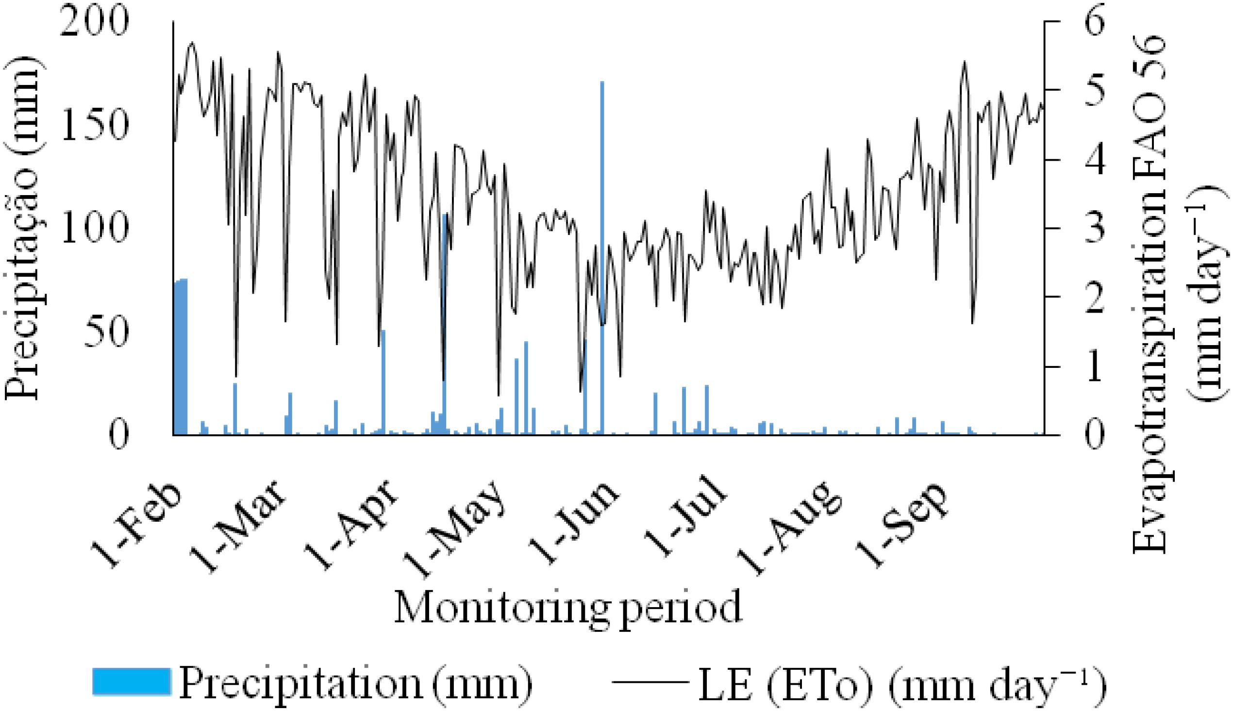
Figure 2 shows the average daily variation of Qg over the monitoring period. The highest and lowest average value of Qg was observed on February 5 and May 5, respectively, concomitantly to precipitation and cloudiness variation, allowing characterizing the days of clear (27.8 MJ m^-2 day^-1) and cloudy (4.58 MJ m^-2 day^-1) sky.

FIGURE 2
Variation of the average global solar radiation (Qg) and accumulated daily precipitation (B) over the monitoring period.

The accumulated total precipitation was 862 mm over the monitoring period, which means an intense precipitation associated with a low solar radiation availability. On May 30, the accumulated precipitation in only 6 hours was 170 mm, which represents 19.7% of the total period (Figure 2). According to INPE (2017), episodes of easterly wave disturbances (EWD) favored excessive rainfall between the states of Parana and Pernambuco in May 2016. However, total precipitation was lower than the historical average for almost all the eastern band of the Northeast region.

Rn values ranged from 5.71 to 37.87 MJ m^-2 day^-1, with an average of 22.82 MJ m^-2 day^-1. LE values ranged from 1.15 to 20.83 MJ m^-2 day^-1, with an average of 5.21 MJ m^-2 day^-1. The lowest LE values are due to cloudiness with low levels of global solar radiation (Figure 3). H values ranged from −0.21 to 30.87 MJ m^-2 day^-1, with an average of 17.38 MJ m^-2 day^-1, while G presented an average value of 0.23 MJ m^-2 day^-1, ranging from 0.05 to 0.37 MJ m^-2 day^-1.

FIGURE 3
Daily variation of the energy balance components net balance (Rn), sensible heat flux (H), latent heat flux (LE), and soil heat flux (G) over the monitoring period on the non-vegetated slab.

The variation of monthly average daily values of H and LE measured in the non-vegetated slab is shown in Figure 4. H presented the highest monthly value in February (22.82 MJ m^-2 day^-1) and the lowest monthly value in June (12.28 MJ m^-2 day^-1). In addition, the highest LE value was observed in April (6.55 MJ m^-2 day^-1) and the lowest LE value was observed in September (6.55 MJ m^-2 day^-1). Over the monitoring period, energy demand for LE was higher than that observed for H, with minimum values at the beginning of the rainy season gradually increasing until reaching the maximum values in the dry season.

FIGURE 4
Monthly variation of the average values of sensible (H) and latent (LE) heat fluxes over the monitoring period in the non-vegetated slab.

The variation of evapotranspiration and precipitation over the experimental period on the simulated green roof is shown in Figure 5. The average daily evapotranspiration was 3.57 mm day^-1, with a minimum of 0.60 mm day^-1 in May and a maximum of 5.87 mm day^-1 in February, which is due to a higher Qg availability and a high Tair. These results are in accordance with those found by Machado et al. (2016) in Cuiabá, MT, who observed a maximum evapotranspiration of 5.7 mm day^-1 in the undergrowth vegetation area.

FIGURE 5
Precipitation (mm) and average evapotranspiration (LE) (mm day^-1) over the monitoring period on the simulated green roof.

Regarding the energy balance components in the simulated green roof, Rn values ranged from 0.64 to 17.11 MJ m^-2 day^-1 over the monitoring period (Figure 6). These values are in accordance with those found by Oliveira (2012), who analyzed the energy balance in a pasture area in Tapacurá, PE, and found Rn values between 1.2 and 16.5 MJ m^-2 day^-1.

FIGURE 6
Daily variation of the energy balance components net radiation (Rn), sensible heat flux (H), latent heat flux (LE), and soil heat flux (G) over the monitoring period on the simulated green roof.

Figure 6 shows that the minimum and maximum H values were −2.79 and 3.21 MJ m^-2 day^-1, respectively. LE values varied from 1.48 to 14.38 MJ m^-2 day^-1.

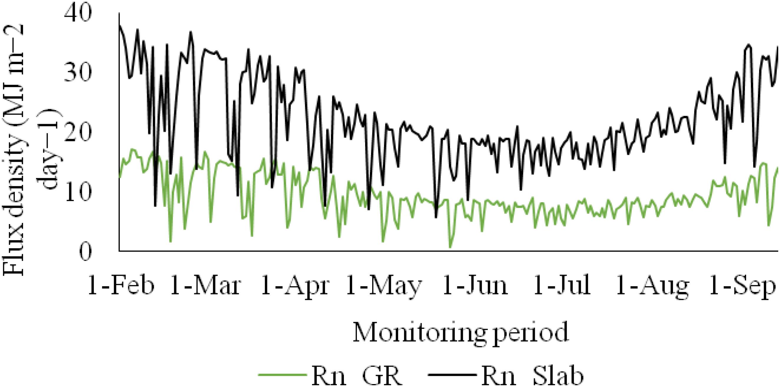
The average monthly net radiation in February presented the highest values for slab and simulated green roof (29.47 and 12.98 MJ m^-2 day^-1, respectively) (Figure 7). In general, Rn values are slightly higher when compared to those observed in adjacent rural regions due to the combined effect of short- and longwave radiation (Callejas et al., 2012). Brest (1987) pointed out that the presence of vegetation in urban areas reduced net radiation on the surface mainly because the effective albedo of a vegetated surface was higher than that found on a surface without vegetation.

FIGURE 7
Daily variation of net radiation (Rn) over the monitoring period on the slab and simulated green roof (GR).

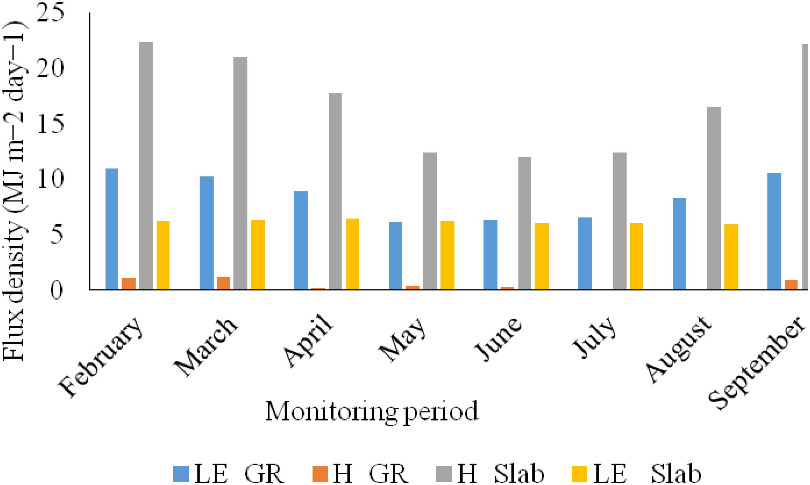
Over the monitoring period, H on the simulated green roof was lower than that observed on the slab, i.e. presented values of 1.29 and 22.82 MJ m^-2 day^-1 in February, 1.36 and 21.45 MJ m^-2 day^-1 in March and 18.15 MJ m^-2 day^-1 in April, 0.55 and 12.70 MJ m^-2 day^-1 in May, 0.41 and 12.28 MJ m^-2 day^-1 in June, 0.11 and 12.71 MJ m^-2 day^-1 in July, 0.22 and 16.81 MJ m^-2 day^-1 in August, and 1.15 and 22.59 MJ m^-2 day^-1 in September for the simulated green roof and slab, respectively (Figure 8).

FIGURE 8
Monthly variation of latent (LE) and sensible (H) heat fluxes over the monitoring period on the simulated green roof (GR) and slab.

When analyzing areas with and without vegetation in a city of southern Ceara State, Arraes et al. (2012) observed that vegetation removal resulted in an increased H, which reinforces the energy flux effect on the air heating in urban areas.

LE presented higher values for the simulated green roof over the monitoring period, except in May. The highest variation between simulated green roof and slab was observed in February (4.94 MJ m^-2 day^-1) and September (4.89 MJ m^-2 day^-1) due to the high Qg availability (Table 1). In contrast, the lowest difference between LE in the simulated green roof and slab was observed in May (0.07 MJ m^-2 day^-1).

In terms of percentages, H was the dominant term in the slab over the analyzed period, corresponding to 75% of the energy balance. LE corresponded to 22% over the monitoring period. Because it is a concrete surface and due to its thermal characteristics such as low thermal resistance and high thermal capacity (Laberts et al., 2014), G corresponded to 3% (Figure 9A). In the simulated green roof (Figure 9B), H, LE, and G corresponded, respectively, to 7, 87, and 7% of the energy balance.

FIGURE 9
Percentage variation of soil (G), sensible (H), and latent (LE) heat fluxes on the slab (A) and simulated green roof (B).

CONCLUSIONS

Simulation model allowed determining the energy balance for the green roof, being determined and quantified modifications in the micrometeorological elements with a consequent change in the energy balance.

Energy balance for the simulated green roof indicated that the sensible heat flux was 69% lower than that observed for the slab and 55% higher for the latent heat flux.

ACKNOWLEDGMENTS

To CAPES - Coordination for the Improvement of Higher Level Personnel for granting the scholarship and to the Construtora Rio Ave for the partnership and providing the experimental area to conduct this research.

REFERENCES

• APAC - Agencia Pernambucana de Águas e Clima. Informe climático de junho de 2016. Available in: http://www.apac.pe.gov.br/arquivos_portal/informes/Informe_Climatico_junho_2016.pdf Accessed: Jan 20, 2017.
  » http://www.apac.pe.gov.br/arquivos_portal/informes/Informe_Climatico_junho_2016.pdf
• APAC. Available in: http://www.apac.pe.gov.br/meteorologia Accessed: Jan 21, 2017.
  » http://www.apac.pe.gov.br/meteorologia
• Arraes FDD, Andrade EM, Silva BB (2012) Dinámica do balanço de energia sobre o agude Orós e suas adjacências. Revista Caatinga 25(1):119-127.
• Brest CL (1987) Seasonal albedo of an urban/rural landscape from satellite observations. Journal of Climate and Applied Meteorology 26:1169-1187.
• Callejas IJA, Durante LC, Oliveira AS, Nogueira MCJA (2012) Uso do solo e Temperatura Superficial em Área Urbana. Mercator 10(23):207-223.
• Emmanuel R, Loconsole A (2015) Green infrastructure as anadaptation approach totacklingurbanoverheating in the Glasgow Clyde Valley Region, UK. Landscape Urban and Planing 138:71-86.
• Fanaya Júnior ED, Lopes AS, Jung LH, Oliveira GQ (2012) Métodos empíricos para estimativa da evapotranspiração de referência para Aquidauana-ms. Irriga 17(4):418-434.
• Jenerette GD, Harlan SL, Buyantuev A, Stefanov WL, Declet-Barreto J, RuddellBL, Myint SW, Kaplan S, Li X (2016) Micro-scale urban surface temperatures are related to land-cover features and residential heat related health impacts in Phoenix, AZ USA, Landscape Ecology 31(4):45-760.
• Gargari C, Bibbiani C, Fantozzi F, Campiotti CA (2016) Simulation of thethermal behavior of a building retrofitted with a green roof: optimization of energy efficiency with reference to Italian climatic zones. Agriculture and Agricultural Science Procedia 8:628-636.
• Gunawardena K R, Wells M J, Kershaw T (2017) Utilising green and bluespace to mitigate urban heat island intensity. Science of the Total Environment 584:1040-1055.
• INMET - Instituto Nacional de Meteorologia (2016) Banco de dados meteorológicos. Available in: http://www.inmet.gov.br/portal/index.php?r=empo/graficos Accessed in: Jun 1, 2016.
  » http://www.inmet.gov.br/portal/index.php?r=empo/graficos
• INPE - Instituto Nacional de Pesquisas Espaciais (2017) Boletim de Prognóstico Climático. INPE/PROGCLIMA. Available in: http://infoclima1.cptec.inpe.br/index_prog.shtml Accessed: Jan 22, 2017.
  » http://infoclima1.cptec.inpe.br/index_prog.shtml
• Laberts R, Dutra L, Pereira FOR (2014) Eficiencia energética na arquitetura. Rio de Janeiro, ELETROBRAS/PROCEL, 3ed. 366p.
• Machado NG, Biudes MS, Angelini LP, Souza DMS, Nassarden DCS, Bilio RS, Silva TJ, Neves GAR, Arruda PHZ, Nogueira JS (2016) Sazonalidade do Balanço de Energia e Evapotranspiração em Área Arbustiva Alagável no Pantanal Mato-Grossense. Revista Brasileira de Meteorologia 31(1):82-91.
• Oliveira IA (2012) Balanço de Energia em área urbana na cidade de Recife-PE. Tese, Departamento de Energia Nuclear, Universidade Federal de Pernambuco.
• Pereira AR, Angelocci LR, Sentelhas PC (2002) Agrometeorologia: fundamentos e aplicações práticas. Guaíba, Agropecuária, 478p.
• Qiu GY, Li HY, Zhang QT, Chen W, Liang XJ, Li XZ (2013) Effects of evapotranspiration on mitigation of urban temperature by vegetation and urban agriculture. Journal of Integrative Agriculture 12:1307-1315.
• Santana NC (2014) Investigação de Ilhas de Calor em Brasilia: Análise Multitemporal com Enfoque na Cobertura do Solo. Revista Brasileira de Geografia Fisica 7:1030-1044.
• Stewart ID, Oke TR (2012) Local climate zones for urban temperature studies. Bulletin of the American Meteorological Society 93(12):1879-1900.

Publication Dates

• Publication in this collection
  May-Jun 2018

History

• Received
  31 Oct 2017
• Accepted
  05 Apr 2018