
Abstract
In the present paper we discuss the development of "wave-front", an instrument for determining the lower and higher optical aberrations of the human eye. We also discuss the advantages that such instrumentation and techniques might bring to the ophthalmology professional of the 21st century. By shining a small light spot on the retina of subjects and observing the light that is reflected back from within the eye, we are able to quantitatively determine the amount of lower order aberrations (astigmatism, myopia, hyperopia) and higher order aberrations (coma, spherical aberration, etc.). We have measured artificial eyes with calibrated ametropia ranging from +5 to -5 D, with and without 2 D astigmatism with axis at 45º and 90º. We used a device known as the Hartmann-Shack (HS) sensor, originally developed for measuring the optical aberrations of optical instruments and general refracting surfaces in astronomical telescopes. The HS sensor sends information to a computer software for decomposition of wave-front aberrations into a set of Zernike polynomials. These polynomials have special mathematical properties and are more suitable in this case than the traditional Seidel polynomials. We have demonstrated that this technique is more precise than conventional autorefraction, with a root mean square error (RMSE) of less than 0.1 µm for a 4-mm diameter pupil. In terms of dioptric power this represents an RMSE error of less than 0.04 D and 5º for the axis. This precision is sufficient for customized corneal ablations, among other applications.
Optical aberrations; Corneal topography; Zernike polynomials; Refractive surgery
Braz J Med Biol Res, November 2002, Volume 35(11) 1395-1406
Measuring higher order optical aberrations of the human eye: techniques and applications
L. Alberto V. Carvalho1, J.C. Castro1 and L. Antonio V. Carvalho2
1Grupo de Óptica, Instituto de Física de São Carlos, Universidade de São Paulo, São Carlos, SP, Brasil
2Departamento de Matemática, Universidade Estadual de Maringá, Maringá, PR, Brasil
References
Abstract
In the present paper we discuss the development of "wave-front", an instrument for determining the lower and higher optical aberrations of the human eye. We also discuss the advantages that such instrumentation and techniques might bring to the ophthalmology professional of the 21st century. By shining a small light spot on the retina of subjects and observing the light that is reflected back from within the eye, we are able to quantitatively determine the amount of lower order aberrations (astigmatism, myopia, hyperopia) and higher order aberrations (coma, spherical aberration, etc.). We have measured artificial eyes with calibrated ametropia ranging from +5 to -5 D, with and without 2 D astigmatism with axis at 45º and 90º. We used a device known as the Hartmann-Shack (HS) sensor, originally developed for measuring the optical aberrations of optical instruments and general refracting surfaces in astronomical telescopes. The HS sensor sends information to a computer software for decomposition of wave-front aberrations into a set of Zernike polynomials. These polynomials have special mathematical properties and are more suitable in this case than the traditional Seidel polynomials. We have demonstrated that this technique is more precise than conventional autorefraction, with a root mean square error (RMSE) of less than 0.1 µm for a 4-mm diameter pupil. In terms of dioptric power this represents an RMSE error of less than 0.04 D and 5º for the axis. This precision is sufficient for customized corneal ablations, among other applications.
Key words: Optical aberrations, Corneal topography, Zernike polynomials, Refractive surgery
Introduction
The ophthalmology professional of the 21st century is living a silent revolution, one which started at the University of Heidelberg (1994) with the Ph.D. thesis of Liang (1). Many scientists throughout the history of physiological optics have attempted to precisely measure the optical aberrations of the human eye (2). Scheiner in 1619 (3), published the work "Oculus, sive fundamentum opticum" where he announced the invention of a disc with a centered and a peripheral pinhole that was placed before the eyes of a subject to view a distant light source (Figure 1). If the subject saw a single spot he was an emmetrope, if he saw two inverted spots, he was a myope and if he saw two upright spots, a hyperope. This device was the first qualitative refractor and became known as Scheiner's disc. After Scheiner, many scientists attempted to construct more precise refractors. Tscherning (4) in 1894 used a four-dimensional spherical lens with a grid pattern on its surface to project a regular pattern on the retina (Figure 2). He would then ask the patient to sketch drawings of the pattern. Depending on the pattern's distortion, Tscherning was able to obtain a semiquantitative measurement of the patient's aberrations. It was only at the beginning of the 1960s that Howland (5) devised a quantitative version of the Tscherning aberroscope by attaching an imaging system and implementing rigorous mathematical analysis of the collected data. Of course, low resolution quantitative systems (autorefractors) have been developed in parallel throughout the last quarter of the last century. We will not discuss the principle of these instruments here, which has been recently reported elsewhere (6-9), but we will compare the precision of our results with those of autorefractors in general.
The instruments devised by Scheiner, Tscherning and later by Howland, all had a specific disadvantage. They were developed in a "non-computerized age". Although there were computers back in the 1960s, the microcomputer "revolution" started only in the mid-1980s. The same occurred with the devices for measuring corneal curvature (videokeratoscopes). Although Plácido (10) developed the technique still used nowadays more than a century ago other devices with magnifying optics and photographic cameras were only possible later in the 20th century. These improvements culminated in the development of well-known keratometers and the photokeratoscope. But these were still limited techniques. The keratometer is still used today, but it only measures the steepest and the flattest meridians at the central 3 mm of the cornea; the photokeratoscope photographs had to be developed and analyzed manually, a process that could take hours, if not days. And even after a careful analysis, few techniques were available for displaying these results in a comprehensive and compact fashion. There were no fast methods for Scientific Visualization (11) (a term referring to a relatively new field in computer graphics, initiated in the mid-1980s, with the objective of developing more didactic techniques for visual presentation and analysis of scientific data). Since the mid-1980s, with the microcomputer "revolution", computer power became accessible enough so as to be incorporated into traditional photokeratoscopes. Thus, the photokeratoscope became the modern computerized videokeratoscope, which is an example of the improvement allowed by the integration of computers and medical devices. The photographic cameras were replaced by modern semiconductor charge coupling devices (CCD) and the tiresome analysis of the Plácido images was replaced by fast and semiautomated image processing algorithms (12,13) and sophisticated mathematical models of the human cornea (14,15). Nowadays the whole process of corneal analysis takes only a few seconds and at the end the eye-care professional may have a multitude of visualization options at a click of the mouse, with the aid of special tools, such as indexes for keratoconus screening (16,17), contact lens fitting modules (18) and special displays of corneal parameters (19). These displays may go from simple corneal slices, difference maps for pre- and postsurgical analysis, up to rotating three-dimensional corneal maps.
It is our very strong belief that the refraction techniques available nowadays have many limitations, analogous to the photokeratoscopes back in the 1950s. Although the conventional autorefractors available today have sophisticated accommodation devices and electronics, like linear CCD for signal processing and microprocessors for dedicated tasks, they still measure refractive errors in only three meridians. The output is usually on a sheet of paper with two lines or a few more, indicating the ametropia in the conventional spherocylindrical form: sphere + cylinder at axis. Until today, the autorefraction and the conventional trial lens procedure have been sufficiently precise to prescribe spectacles and contact lenses, and patients have been reasonably satisfied. With the advent of refractive surgery and the possibility of contact lenses with customized anterior shapes, the conventional refraction instrumentation is no longer precise enough. And this precision has no relation to how precisely these instruments can measure the best spherocylinder surface that approximates the eye's ametropia; it is the lack of resolution that makes these instruments obsolete for modern applications. For customized corneal ablation there is an intrinsic need to know the refractive errors at several points over the entrance pupil. This happens because the modern laser beams (20) have enough resolution to independently ablate specific regions of the cornea.
In fact, although there have been low priced computers since the mid-1980s, no quantitative technique for measuring eye aberrations with high resolution was applied until 1994. Liang et al. (1) applied to the human eye an idea originally applied to general optical instruments such as astronomical telescopes since the 1950s (21). Because of atmospheric turbulence and subtle changes in air temperature, astronomical images are usually composed of several optical aberrations, which cause considerable image degradation, preventing astronomers from performing a thorough analysis of these images. In order to diminish or eliminate these effects, a field of optics, called Adaptive Optics (22), studies methods for measuring and compensating for these aberrations. The sensor used to measure these aberrations was first developed by Hartmann in 1900 (23) and later improved by Shack in 1971 (24). This sensor became known as the Hartmann-Shack sensor, abbreviated HS sensor.
We present here the development and preliminary results obtained with an HS sensor constructed at the Instituto de Física de São Carlos, USP (25), that was used to measure artificial eyes with different aberrations. Our claim is that the HS sensor may be applied to the human eye with more precision than traditional refraction techniques.

[View larger version of this image (14 K JPG file)]

[View larger version of this image (17 K JPG file)]
Material and Methods
Optical configuration
The diagram in Figure 3 shows a simplified scheme of the instrument.
A fiber optic infrared light source generates a non-coherent bundle of rays which are collimated by a system of lenses and a diaphragm. This small diameter (0.5 mm) bundle of rays enters the eye through the optical center of the entrance pupil. This bundle of rays focuses a small spot over the retina because of very little refraction and negligible aberration. The diffuse reflection at the eye fundus generates a cone of light rays that leaves the retina in the direction of the lens and pupil. The light rays that leave the eye hit a beam splitter and a set of relay lenses. After that, they go through a set of micro-lenses which compose the HS sensor (Figure 4). The HS sensor is simply an array of uniformly distributed very small lenses analogous to those of an insect eye (such as the Drosophila fly). There are many possible sizes and configurations for HS sensors (26). Our "home-made" HS sensor is composed of a grid of 15 x 15 micro-lenses. At the focal plane of the micro-lens array there is a high sensitivity monochromatic CCD. We explain the HS principle in the diagram in Figure 5. For a plane wave-front the focusing position on the CCD plane is exactly at the intersection of the axis of the micro-lens with the CCD plane; on the other hand, for an aberrated wave-front, light focuses on a slightly shifted spot. For a set of micro-lenses the same principle applies and we will have uniformly spaced spots for a plane wave and non-uniformly distributed points for aberrated waves. The amount of displacement of the spots permits us to determine the exact amount of wave-front aberration. We will present the mathematical procedures in the "Calculating optical aberrations from Zernike polynomials" subsection. In Figure 6 we present an example of an HS image obtained for an artificial eye calibrated with zero dioptric power (no aberrations).

Optical configuration used to measure optical aberrations of the eye. An infrared source [1] with 200 µW is focused towards the eye through spherical lenses [6] and [16]. A filament light source [5] is used to illuminate a light diffuser, which is attached to a reticule containing a balloon picture [4] (this is simply a psychological advantage that calls the patient's attention during accommodation). This accommodation system shall be tested during the second phase of this project, in which measurements will be made on human eyes. The image formed by lens [3] and beam splitter [2] is located at a far point from the patient in order to induce the accommodation of the crystalline. Approximately 1% of the incident light scattered at the back of the eye (retina) is reflected back to the beam splitter [7], goes through spherical lenses [8] and [9], a stop [10] located at the focal point of lenses [9] and [11] for elimination of undesired reflections at the cornea [17] and finally hits the Hartmann-Shack (HS) sensor [12]. A charge coupling device (CCD) [13] is placed on the focal plane of the HS micro-lenses, and attached to a "frame-grabber" [14] installed in an IBM compatible computer, where the HS images are processed [15] and the optical aberration is calculated.
[View larger version of this image (23 K JPG file)]
 E, width and height; A, depth of the non-lenticular base; D, depth of each micro-lens; R, radius of each micro-lens, and C, micro-lens diameter.
[View larger version of this image (41 K GIF file)]
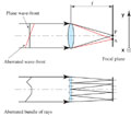 Upper diagram, A plane wave-front hits a single micro-lens and focuses at a point P located over the optical axis and at a distance f from the lens; for the same micro-lens an aberrated wave-front focuses at point A, also on the focal plane but shifted away from the optical axis. Lower diagram, For a set of micro-lenses, an aberrated wave-front will focus on unevenly spaced points (shifted away from the optical axis of each micro-lens) over the focal plane. It is the quantification of the individual shifts that allows one to determine the local slopes of the wave-front and then, from this information, retrieve the entire wave-front surface. The x,y arrows to the right of the upper diagram show the coordinate system directions (y is pointing upwards and x is coming outside from the page) used according to Equations 7 and 8.
[View larger version of this image (34 K JPG file)]

Hartmann-Shack image obtained with our instrument for an artificial mechanical eye calibrated with no aberration (zero diopter), i.e., emmetropic.
[View larger version of this image (111 K JPG file)]
Image processing
In order to calculate the wave-front aberration, we must extract the information on the Cartesian positions of each spot from the digitized images using image processing techniques (12,13). The image processing of the HS patterns is the first step towards the quantification of aberration. We start by digitizing the HS image in Windows bitmap 8 bit format with an IBM compatible computer with a Pentium III 800 MHz Intel processor. This is accomplished with an attached frame-grabber (model Meteor, Matrox Electronic Systems, St. Regis Dorval, Quebec, Canada). The goal is to find the "center of mass" of each spot. We start by analyzing the distribution of gray levels for horizontal and vertical lines along the image. From this distribution we determine a set of grids in such a way that each cell contains a spot. From the gray level distribution inside each cell we determine the centroid of the spot by using equations:
(Equation 1)

(Equation 2)
where m and n are the horizontal and vertical pixels inside the considered cell, x and y are the horizontal and vertical positions of the pixel in mn, and g is the intensity of gray level in an 8-bit gray scale image (0 means totally black and 255 means totally white).
Column A in Figure 7 shows the results of image processing for all calibrated aberrations, with centroids marked with a cross. As stated before, from the difference in centroid position for a plane wave and an aberrated wave, it is possible to calculate the wave-front aberration (commonly called the wave-front function and represented by W) using special polynomials called Zernike polynomials (27) and mean square interpolation. We will now describe the mathematical procedures used for this purpose.
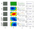 A, Hartmann-Shack (HS) images for all five aberrations showing HS spots with superimposed "centers of mass" (gray crosses) detected by our image processing algorithm. B, Two-dimensional view of the wave-fronts calculated from the Zernike coefficients retrieved from the HS spots in A and from Equations 6 to 13. C, Same as in B, but plotted as three-dimensional (x, y, z) graphs. D, Zernike coefficient values for each aberration. Notice that for the plane wave-front they are all zeros, as expected. These are the Zernike coefficients which are added to Equation 9 in order to retrieve the wave-fronts plotted in B and C.
[View larger version of this image (68 K JPG file)]
Calculating optical aberrations from Zernike polynomials
Although Seidel polynomials are extensively used in the description of optical aberrations they have certain limitations that are not present in Zernike polynomials (see a list of the first 15 Zernike polynomials in Table 1). The five conventional Seidel aberrations are classified as spherical aberration, coma, astigmatism, curvature of field (or focus shift), and distortion (or tilt). If we look carefully at Table 1, we may see that terms 13, 8 and 9, 4 and 6, 5, 2 and 3, correspond, respectively, to the Seidel aberrations. So this is the first advantage: the Seidel aberrations are contained in the Zernike polynomials; another advantage is that the Zernike polynomials form a complete and normalized set of functions over the unit circle (x2 + y2£1) and also have certain properties of invariance which are desirable in terms of symmetry and mathematical elegance, i.e., simplicity. Since a thorough and detailed discussion of Zernike polynomials and its properties is not within the scope of this article, we address the reader to what is, to our knowledge, one of the most complete discussions on the subject: appendix VII of Ref. 27, pages 905-910. We next describe some basic aspects of these polynomials. Zernike polynomials are a set of maps in the z-axis with domain at the unit disc x2 + y2£1 of the x,y-plane, which have the desirable property that their combinations can be found to fit well the surface shapes of reasonably "well-behaved" (28) wave-front aberrations. In polar coordinates, Zernike polynomials are the product of a radial polynomial and an azimuthal map:
(Equation 3)
where l may be any integer number and n may be any positive integer and zero. When l is greater than or equal to zero, the sine function is used and when it is smaller than zero the cosine function is used. The radial components of the Zernike polynomials are given by:
(Equation 4)
The Zernike polynomials are thus a set of orthogonal maps defined in the unit circle. Their orthogonallity condition is expressed by:

where d is the Kronecker Delta, i.e.,
(Equation 6)
for integer values of p.
The main motivation for using Zernike polynomials is that they describe the shapes of four conventional Seidel aberrations with high precision. Because there is no limit to the number of terms that may be used, many higher order aberrations can be described by Zernike polynomials, among them coma, 3rd order spherical aberration, etc. The choice of exactly how many terms to use has been discussed at a specific meeting (29) of Vision Scientists, and the convention adopted was to use the first 15 Zernike terms, which are shown in Table 1. Actually, this choice is based on the fact that it is enough to use the first 15 linearly independent Zernike polynomials in order to obtain a highly accurate description of the most common aberrations found in human eyes (29). These polynomials, in mathematical terms, comprise a set of linearly independent polynomials in two indeterminates with a degree of 4 or less, which are orthonormal with respect to the inner product given in Equation 5.
We mention in the section "Optical configuration" the possibility of calculating the wave-front aberration from the wave-front slopes. Based on Figure 5, we may write the slopes in the x and y directions as:


where (xa, ya) is the coordinate of a spot from an aberrated wave-front, (xc, yc) is the coordinate of the reference spot, i.e., a non-aberrated, plane wave-front, and f is the focal length of the micro-lenses. If we use a single index k as a function of n and l (the indexes of Equations 3-5), namely,

then we may write the wave-front as:
(Equation10)
and its partial derivatives as
(Equation 11)
(Equation 12)
Note that k is the number of the Zernike term according to Table 1. In order to find the Zernike coefficients for a specific wave-front, we perform a minimum square fit for all i, j centroids which form the HS image. This procedure consists of minimizing the sum (see Equation 13) relative to each Zernike coefficient, and therefore we have to find dS/dCt = 0 for t = 1, ...., k (see Equation 14) from where we extract a square linear system AC = b with k equations and k unknown values of C. By solving this linear system through conventional procedures (LU decomposition and Gaussian elimination method) (30) we find 15 values of C for each measured eye. For a flat wave-front the partial derivatives dW/dx and dW/dy are zero, and we therefore obtain a C = 0 solution, which by the general equation (10) yields W(xij, yij) = 0, a plane wave on the x,y-plane. Now for wave-fronts that are not flat we obtain values of partial derivatives different from zero, and therefore the linear system will not have a trivial solution. The coefficients that contribute most to a specific aberration will have greater values. For example, if the measured eye has a large amount of coma the eighth and ninth coefficients will have higher values than others. In contrast, if there is a greater amount of astigmatism at 45º, the fourth term will predominate. In the next section we show results for several calibrated aberrations on an artificial eye.


Results
Measurements were made on a mechanical (artificial) eye which was calibrated with five different types of ametropia: zero dioptric (D) power, i.e., emmetropic (0 D), hyperopic (+5 D), myopic (-5 D), and 2 D astigmatism with axis at 45º and 90º. Image processing was accomplished separately for each aberration (see Figure 7, column 1) and results were plotted in several different outputs.
In Figure 7, from the left to the right column, we may see results for the image processing, two-dimensional color-coded maps for the wave-front, surface maps and, finally, the Zernike coefficients for each of the 15 terms in Table 1. A qualitative analysis of the first row (0 D) shows regularly spaced dots, a color map with one color, a plane of height zero, and coefficients all with a zero value. This is obviously in accordance with the expected values for a zero dioptric eye, i.e., with no aberrations, therefore resulting in a plane wave leaving the eye.
The same qualitative analysis for the other eyes shows the validity of the results. For example, in the cases of +5 D and -5 D, we know that the wave-front should look like a dome-shaped surface, facing downwards for the myopic and upwards for the hyperopic eye. This is in agreement with the expected shapes of wave-fronts leaving eyes with different low order aberrations (Figure 8).
It is possible to relate the wave-front measurements to those of autorefractors. Regardless of the typical high resolution data of HS, it is still possible to retrieve conventional dioptric power values for the best spherocylinder lens that describes the eye's lower order aberrations. If we consider the spherocylindrical lens as

(Equation 15)
the sphere (fD), cylinder (fA) and axis (a) may be written as:
(Equation 16)
(Equation 17)

(Equation 18)
where d is the diameter of the entrance pupil.
The root mean square errors for the measurements shown in Figure 7 were as follows: 0.04 D for sphere and cylinder and 4º for axis. It is known that autorefractors have typically errors of 0.12 D for sphere and cylinder and 5º for axis. We may see from these preliminary measurements that the wave-front device allows for more precise examination. We believe this precision is reproducible for eyes of the general population (preliminary tests are currently being conducted in our laboratory (31)).
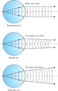
Differently shaped wave-fronts leaving three types of eye: myopic, hyperopic, and emmetropic. This is simply an alternate view of these common eye aberrations, which are usually explained by drawing paraxial rays from outside to inside the eye. Here we do the contrary: a point light source directed at the retina generates a spherical wave-front which leaves the eye. Because the
[View larger version of this image (71 K JPG file)]
Discussion
We have demonstrated the precision of the HS wave-front sensor in measuring optical aberrations of an artificial calibrated eye. Tests on real eyes should be conducted to verify and validate the technique.
One common difficulty of instruments when attempts at measuring refractive errors are made occurs during accommodation. It is not always possible to repeat the measurements with the crystalline lens at exactly the same dioptric power. This certainly makes the reproducibility of these instruments much lower than expected. Our intention here was not to compare the precision of the whole refractive instrumentation and therefore we did not consider accommodation (our artificial eyes do not have a lens). Our intention was to provide insight about how promising the wave-front technique may be when compared to conventional autorefractors in terms of resolution and precision. An accommodating system, when well functioning, may be applied to either type of instrument, permitting absolute precision comparisons for daily measurements in the human population. We are currently building a genuine accommodation device using a micro-controlled moveable optical system, which is electronically controlled by a software through the parallel port interface of an IBM-compatible PC. The principle of this accommodation system is based on the optical diagram shown in Figure 3 (32).
An important factor is the amount of micro-lenses in the HS sensor. If we double the number of micro-lenses in the row and column, the resolution is multiplied by a factor of 4. On the other hand, for highly distorted corneas this might be a disadvantage. In a previous study (33), by implementing computer simulations of HS patterns for several corneal topographies, we have shown that for eyes with severe curvature changes on the corneal surface (such as keratoconus) the HS spots may overlap, reducing the capacity of the software for image processing and data analysis. In these specific cases, conventional trial lens tests with autoprojectors or Snellen tables may still be necessary.
We strongly believe that the wave-front technology represents the next generation of refractors which will gradually replace conventional refractors, much in the same way that computerized corneal topography replaced the traditional keratometer and the photokeratoscope. Moreover, the wave-front will permit precise corneal ablations, resulting in algorithms that may execute what is being called "customized corneal ablations" (34).
Acknowledgments
We would like to thank Dr. Wallace Chamon, Dr. Paulo Schor and Dr. Rubens Belfort Jr., Escola Paulista de Medicina, UNIFESP, for valuable insights.
Address for correspondence: L. Alberto V. Carvalho, Grupo de Óptica, IFSC, USP, 13560-900 São Carlos, SP, Brasil. E-mail: lavcf@ifsc.sc.usp.br
Research partially supported by FAPESP (Nos. 01/03132-8 and 00/06810-4). L. Antonio V. Carvalho is partially supported by CNPq (No. 304041/85-8). Received June 28, 2001. Accepted June 10, 2002.
- 1. Liang J, Grimm B, Goelz S & Bille JF (1994). Objective measurement of wave aberrations of the human eye with the use of a Hartmann-Shack wave-front sensor. Journal of the Optical Society of America, 11: 1949-1957.
- 2. Thibos LN (2000). Principles of Hartmann-Shack aberrometry. Journal of Refractive Surgery, 16: 540-545.
- 3. Scheiner C (1619). Oculus, sive fundamentum opticum. Innspruk, Austria.
- 4. Tscherning M (1894). Die monochromatischen Aberrationen des menschlichen Auges. Zur Physiologischen Psychologie der Sinnesorgane, 6: 456-471.
- 5. Howland B (1960). Use of crossed cylinder lens in photographic lens evaluation. Applied Optics, 7: 1587-1588.
- 6. Campbell FW & Robson JG (1959). High speed infrared optometer. Journal of the Optical Society of America, 49: 268-272.
- 7. Charman WN & Heron G (1975). A simple infra-red optometer for accommodation studies. British Journal of Physiological Optics, 30: 1-12.
- 8. Cornsweet TN & Crane HD (1976). Servo-controlled infrared optometer. Journal of the Optical Society of America, 60: 548-554.
- 9. Shikawa YY (1988). Eye refractive power measuring apparatus. US Patent No. 4755041, July 5.
- 10. Plácido A (1880). Novo instrumento de exploração da córnea. Periodico d'Oftalmologia Pratica, 5: 27-30.
- 11. Oliveira MCF & Minghim R (1997). Uma introdução à visualização computacional. XVI Jornada de Atualização em Informática, Brasília, DF, Brazil, August 2-8, 85-127.
- 12. Gonzalez RC & Woods RE (1992). Digital Image Processing Addison Wesley Publishing Company, Reading, MA, USA.
- 13. Carvalho LA, Silva EP, Santos LER, Tonissi SA, Romão AC & Castro JC (1996). Detecção de bordas de imagens refletidas pela superfície anterior da córnea. III Fórum Nacional de Ciência e Tecnologia em Saúde, Campos de Jordão, SP, Brazil.
- 14. Mandell RB & St Helen R (1971). Mathematical model of the corneal contour. British Journal of Physiological Optics, 26: 183-197.
- 15. Halstead MA, Barsky BA, Klein SA & Mandell RB (1995). A spline surface algorithm for reconstruction of corneal topography from a videokeratographic reflection pattern. Optometry and Vision Science, 72: 821-827.
- 16. Rabinovitz YS (1998). Keratoconus. Survey of Ophthalmology, 42: 297-319.
- 17. Rabinovitz YS & Rasheed K (1999). KISA% index: A quantitative videokeratography algorithm embodying minimal topographic criteria for diagnosing keratoconus. Journal of Cataract and Refractive Surgery, 25: 1327-1335.
- 18. Donshik PC, Reisner DS & Luistro AE (1996). The use of computerized videokeratography as an aid in fitting rigid gas permeable contact lenses. Transactions of the American Ophthalmological Society, 94: 135-143.
- 19. Budak K, Khater TT, Friedman NJ, Holladay JT & Koch DD (1999). Evaluation of relationships among refractive and topographic parameters. Journal of Cataract and Refractive Surgery, 25: 814-820.
- 20. Carvalho Luis Alberto V, Castro JC, Chamon W, Schor P & Carvalho Luis Antonio V (2001). Wave-front measurements of the human eye using the Hartmann-Shack sensor and current state-of-the-art technology for excimer laser refractive surgery. Lasik and beyond Lasik. Chapter 31. In: Boyd BF (Editor), Highlights of Ophthalmology Pergamon Press, Oxford, England.
- 21. Babcock HW (1953). The possibility of compensating astronomical seeing. Publications of the Astronomical Society of the Pacific, 65: 229 (Abstract).
- 22. Tyson RK (1997). Principles of Adaptive Optics 2nd edn. Academic Press, San Diego, CA, USA.
- 23. Hartmann J (1900). Bemerkungen über den Bau und die Justierung von Spektrographen. Zeitschrift für Instrumentenkunde, 20: 47.
- 24. Shack RV & Platt BC (1971). Production and use of a lenticular Hartmann screen. Journal of the Optical Society of America, 61: 656.
- 25. Junior FS, Yasuoka F, Santos J, Carvalho LA & Castro JC (2001). Desenvolvimento de um sistema para medidas de aberrações ópticas do olho humano usando a técnica de Hartmann-Shack. XXIV Encontro Nacional de Física da Matéria Condensada, Óptica (Lasers e Instrumentação Óptica), São Lourenço, MG, Brazil, May 15-19, 457.
- 26. Geary JM (1995). Introduction to wave-front sensors. In: O'Shea DC (Editor), Tutorial Texts in Optical Engineering Vol. TT 18. SPIE Press, New York, NY, USA.
- 27. Born M (1975). Principles of Optics Cambridge University Press, UK (ISBN: 0521642221, 7th edn., October 1999), 464-466.
- 28. Cournant R & Hilbert D (1953). Methods of Mathematical Physics Vol. 1. 1st English Edition. Interscience Publishers, New York, NY, USA.
- 29. Thibos LN, Applegate RA, Schwiegerling JT & Webb R (2000). VSIA Standards Taskforce members. Report from the VSIA taskforce on standards for reporting optical aberrations of the eye. Journal of Refractive Surgery, 16: S654-S655.
- 30. Press WH, Flannery BP, Teukolsky SA & Vetterling WT (1989). Numerical Recipes in Pascal - the Art of Scientific Computing Cambridge University Press, Cambridge, UK, 37-39.
- 31. Santos JB, Scannavino Jr FA, Carvalho LAV, Filho RL & Castro JCN (2001). Sensor Hartmann-Shack para uso oftalmológico. XXIV Encontro Nacional de Física da Matéria Condensada, Óptica (Lasers e Instrumentação Óptica), São Lourenço, MG, Brazil, May 15-19, 457.
- 32. Scannavino Jr FA, Filho RL, Santos JB, Carvalho LAV & Castro JCN (2001). Instrumento eletro-óptico para medidas automatizadas da acomodação do olho humano (in vivo) durante medidas refrativas. XXIV Encontro Nacional de Física da Matéria Condensada, Óptica (Lasers e Instrumentação Óptica), São Lourenço, MG, Brazil, May 15-19, 458.
- 33. Carvalho LA, Castro JC, Schor P & Chamon W (2000). A software simulation of Hartmann-Shack patterns for real corneas. International Symposium: Adaptive Optics: From Telescopes to the Human Eye Murcia, Spain, November 13-14.
- 34. Klein SA (1998). Optimal corneal ablation for eyes with arbitrary Hartmann-Shack aberrations. Journal of the Optical Society of America, 15: 2580-2588.
Correspondence and Footnotes

Publication Dates
-
Publication in this collection
05 Nov 2007 -
Date of issue
Nov 2002
History
-
Accepted
10 June 2002 -
Received
28 June 2001
