
ABSTRACT
Previous work has established that an appreciation of the real effective exchange rate (REER) contributes to premature deindustrialization, less productive investment and dependence on commodity booms and busts in emerging markets economies (EME). From the literature, it is less clear, however, what the most important drivers for the cyclical REER movements in EME are. The aim of this study is to provide empirical evidence about the determinants of the REER movements of 15 emerging markets during the last two decades, using statistical analysis and a dynamic panel fixed effects model approach. Our analysis shows that although “commodity” and “industrial” EME are heterogeneous, REER volatility tends to be higher among the former. EME that had more stable REER fared better than those that had a depreciating or appreciating trend (with the notable exception of China). As theoretically expected, commodity prices are an important structural driver of REER movements in “commodity EME”. Moreover, the results confirm the existence of the Harrod-Balassa-Samuelson effect, and show the importance of financial inflows. Further, the interventions of central banks were partially successful to avoid more substantial appreciations (depreciations). Finally, we find that lower country risk and, at least in some periods, growing broad money in OECD countries has led to REER appreciations in our sample countries.
KEYWORDS:
Real exchange rate; foreign exchange rate policy; commodity prices; capital inflows; global risk
RESUMO
Trabalhos anteriores estabeleceram que uma apreciação da taxa de câmbio efetiva real (REER) contribui para a desindustrialização prematura, investimento menos produtivo e dependência de ciclos de expansão e contração de commodities nas economias de mercados emergentes (EME). Na literatura, é menos claro, no entanto, quais são os fatores mais importantes para os movimentos cíclicos de REER no EME. O objetivo deste estudo é fornecer evidências empíricas sobre os determinantes dos movimentos REER de 15 mercados emergentes nas últimas duas décadas, usando análise estatística e uma abordagem de modelo de efeitos fixos em painel dinâmico. Nossa análise mostra que, embora EME “commodity” e “industrial” sejam heterogêneos, a volatilidade do REER tende a ser maior entre os primeiros. EME que tiveram REER mais estáveis se saíram melhor do que aqueles que tiveram uma tendência de depreciação ou valorização (com a exceção notável da China). Como teoricamente esperado, os preços das commodities são um importante fator estrutural dos movimentos do REER no “EME das commodities”. Além disso, os resultados confirmam a existência do efeito Harrod-Balassa-Samuelson e mostram a importância dos ingressos financeiros. Além disso, as intervenções dos bancos centrais foram parcialmente bem-sucedidas para evitar apreciações mais substanciais (depreciações). Por fim, descobrimos que o menor risco país e, pelo menos em alguns períodos, o aumento de dinheiro nos países da OCDE levaram a apreciações de REER em nossos países da amostra.
PALAVRAS-CHAVE:
Taxa de câmbio real; política de taxa de câmbio; preços de mercadorias; entrada de capital; risco global
INTRODUCTION
Real effective exchange rates (REER) are considered as indicators for the average price competitiveness of all firms of an economy. Emerging Market Economies (EME) are considered here middle-income countries which are in transition to advanced countries but still incorporate many features of developing countries. Their price - and non-price competitiveness needs to improve in order to catch-up with advanced countries. Hence, their REER seems to be important for further development. Standard development economics and growth theories more or less ignore the role of exchange rates for development and growth. Yet, there is widespread agreement that overvalued REER hamper growth, in many cases even persistently.
Most prominently, the theoretical framework of “New Developmentalism” holds that overvalued REER, temporarily or chronically, are a key determinant of underdevelopment, because they hamper investment, industrialisation, technical progress and growth. For promoting industrialisation (or reverting premature deindustrialisation) an “industrial REER” is required; i.e., a stable reduced value of the currency compared to the commodity currency value (Bresser-Pereira, 2019Bresser-Pereira, L.C. (2019). “From classical developmentalism and post-Keynesian macroeconomics to new developmentalism”. Brazilian Journal of Political Economy, 39(2): 187-210.). However, a closer look shows that EME are a quite diverse group of countries and the role of REER for growth and development is not clear-cut. In this paper, we want to shed more light on these issues1 1 Please see Goda & Priewe (2019) for a more detailed description of the main tenets of “New Developmentalism” regarding exchange rates issues, and an extended overview on the existing literature regarding exchange rates in EME. .
Let us first clarify the key terms, REER and EME. REER are defined as inflation-adjusted nominal exchange rates against the main trading partners. Traditional exchange rate theories hold that the real equilibrium exchange rate is determined by absolute or relative purchasing power parity (PPP), which is measured with prices for tradables under competitive conditions (adjusted for transaction costs). Alternatively, the equilibrium nominal exchange rate (NER) gravitates towards nominal interest rate parity (IRP), whereby idiosyncratic country risks have to be accounted for. Deviations stem mainly from expectations regarding future interest rates and country risks.
The term EME was initially invented as a group of developing countries capable to absorb commercial financial inflows from first-world financial investors. The term has never been clearly defined and is often used arbitrarily; it often includes countries like Korea, Hong Kong, Taiwan or Israel, which we consider on all counts developed. Here we adapt the term for a sample of 15 mainly upper middle-income countries, which comprises seven countries from Asia, seven from Latin America, and South Africa. These countries account for 29% of world GDP and 84% of middle-income countries’ GDP (WDI, 2019).
Graph 1 shows that, from our sample, India, Indonesia and the Philippines are classified by the World Bank as lower middle-income countries (below the threshold of US$ 3,895) and Chile and Argentina as high-income countries (not far above the threshold of US$ 12,055). China, India and Indonesia performed with the highest GDP-growth in the period 1996-2016, while Argentina, Brazil and South Africa had the lowest growth (around 2.5% p.a.). Graph 2 shows that China is by far the largest country in our sample (accounting for over 50% of the total GDP of all sample countries), followed by India (10%), Brazil (8%), Russia (6%) and Mexico (5%). All of these data illustrate the heterogeneity of this country group.
The remainder of this paper tries to unravel the main determinants of recent REER movements in the 15 EME of our sample. To achieve this aim, we use first descriptive statistical analysis and then dynamic panel fixed effects regression. This contribution is important insofar existing research has left many questions open regarding EME. These questions comprise mainly the following issues:
-
Are the REER over the long haul of two decades by and large stable, with ups and downs, or is there in some countries a clear upward or downward trend?
-
In what way does the REER of “industrial EME” differ from that of “commodity EME”? Are the REER of “industrial EME” more stable?
-
Are the REER of advanced countries more stable than that of EME? Does the REER of the group of “commodity EME” co-move with the REER of the three main advanced commodity producers Australia, New Zealand and Norway?
-
In currencies with strong overvaluation episodes, do capital inflows matter? Are there peculiar boom periods with high capital inflows and sudden stop episodes with capital flight?
-
What are the main features of countries with a bad rating and above average rating?
-
Are exchange rate regimes, capital controls, and FX-interventions effective?
What is the role of monetary expansion in advanced countries and global risk perceptions?
This paper addresses these questions, and is structured as follows. In the next section, we present an overview on the literature regarding REER of EME. The third section illustrates key data regarding the 15 EME, using descriptive statistical analysis. The fourth section presents the methodology used to test econometrically the main determinants of the REER in the EME of our sample, and then analyses the regression results. The last section concludes.
THE STATE OF EXCHANGE RATE THEORY ON EME CURRENCIES
Contemporary exchange rate theories, as presented in modern advanced textbooks that incorporate recent research, pay hardly any special attention to developing countries or EME. The traditional approaches to exchange rate determination are based on the monetary, PPP and IRP approach, and elaborate on several variants in each category (see, e.g., Isard, 2008Isard, P. (2008). Exchange Rate Economics. Cambridge: Cambridge University Press .; Pilbeam, 2013Pilbeam, K. (2013). International Finance. Houndsmills, New York: Palgrave Macmillan.). However, the so-called PPP - and forward-premium puzzles have not been solved, i.e., strong and persistent deviations of exchange rates from PPP (with long reversion time) and deviation from covered as well as uncovered IRP. Hence, these theories have not been able to provide robust empirical results that allow exchange rate forecasts that are better than random walk.
Keynesian approaches emphasize the role of expectations, uncertainty and speculation. Behavioural approaches, similar to Keynesian, focus often on microeconomic behaviour and practices of forex traders (“money managers”), often in the form of information seeking activities that feed into the formation of expectations or backward-looking expectation in face of uncertainty for the future combined with herding behaviour. An important offspring of IRP is the portfolio balance approach, which assumes that financial assets differ among countries, so that the same assets are imperfect substitutes due to different currency (including time-varying risk perception and liquidity preferences similar to Keynes’s animal spirits).
Some strands in this area also analyse country-specific risks, which lead to higher risk premia and the existence of a currency hierarchy in the global economy. Besides depreciation risks, elements of country-specific risks relevant for EME (and developing countries in general) are: balance of payments deficits, currency mismatches due to “original sin”, fiscal policy risks regarding public debt in foreign currency, underdeveloped bond markets, fragility of the financial sector and its prudential supervision, inflation risks, and distributional conflicts in face of economic inequality.
Regarding currencies of developing and emerging market currencies, there has been substantial empirical research that has shed light on many aspects. The main peculiarity of developing countries’ currencies is seen in their status as “commodity currency” since most developing countries, including many emerging economies, are predominantly commodity producers. The terms-of-trade fluctuation and related Dutch Disease are the key issues in this part of the literature. Another more recent thematic area focuses on financial flows related to portfolio-balance models and changing risk perception of financial investors in the centres of the world economy. Moreover, post-Keynesian approaches stress the importance of financial flows in the context of carry trade and related derivates (see, e.g., Andrade & Prates, 2013Andrade, R.P. & Prates, D.M. (2013). “Exchange rate dynamics in a peripheral monetary economy: a Keynesian perspective”. Journal of Post-Keynesian Economics, 35(3): 399-416,; Kaltenbrunner, 2015Kaltenbrunner, A. (2015). “A post Keynesian framework of exchange rate determination: a Minskyan approach”. Journal of Post Keynesian Economics, 38(3): 426-448.; Ramos & Prates, 2018Ramos, R.A. & Prates, D.M. (2018). “The Post-Keynesian view on exchange rates: towards the consolidation of the different contributions in the ABM and SFC frameworks”. UNICAMP Texto para Discussão, No. 352.).
Commodity prices and exchange rates
The vast literature on Dutch Disease has identified a clear causal link between natural resource prices and REER. Venables (2016Venables, A.J. (2016). “Using natural resources for development. Why has it proven so difficult?” Journal of Economic Perspectives, 30(1): 161-184.) gives a recent summary of this literature, with the key insight that Dutch Disease countries are conspicuously different from agricultural commodities. He concludes that almost all resource-rich countries with non-renewable sub-soil commodities have suffered low growth in the long-run (besides some high-growth episodes in commodity booms). Dutch Disease based on persistently overvalued REER is a pervasive feature of all these countries, with the notable exception of Botswana, Chile and to some extent Venezuela. The blessing of rich and scarce natural resources is mixed since prices are volatile, crowding-out of non-resource tradeable production - mainly manufacturing- is prevailing, and prudent governance of resource rents is difficult and demanding with regard to institutional capacities.
Venables does not elaborate on the main differences between sub-soil mineral and renewable agricultural resources, but these are clear-cut: the former are much scarcer and allow reaping very high rents; they are often state-owned; global competition is mostly oligopolistic (hence countries are not necessarily price takers); their comparative advantage relative to manufacturing is extreme (making it difficult and extremely ambitious to produce non-resource tradable exports profitably); their price hikes are a multiple of agriculture-based price surges; and, in contrast to agricultural commodities, their prices did not have a declining trend during the last five decades. Therefore, the term Dutch Disease has to be used carefully.
Finally, some recent research argues that the REER may not only be affected by the traditional “spending” and “relocation” effects of Dutch Disease but also by massive inflows of external capital that are used to finance the exploitation of raw materials. More specifically, Bresser-Pereira (2009Bresser-Pereira, L.C. (2009): “The tendency to the overvaluation of the exchange rate”. In Bresser-Pereira, L.C. (ed.): Globalization and Competition. Cambridge: Cambridge University Press, 125-147.) argues that commodity boom related financial inflows can generate an overvaluation of the REER that causes a decline in the industrial sector. This argument is corroborated by studies like Ibarra (2011Ibarra, C.A. (2011). “Capital flows and real exchange rate appreciation in Mexico”. World Development, 39(12): 2080-2090.), Naceur et al. (2012Naceur, S.B., Bakardzhieva, D. & Kamar, B. (2012). “Disaggregated capital flows and developing countries’ competitiveness”. World Development, 40(2): 223-237.), Goda & Torres García and Botta (2017Botta, A. (2017). “Dutch Disease-cum-financialization booms and external balance cycles in developing countries”. Brazilian Journal of Political Economy, 37(3): 459-477.) that show that commodity boom related FDI and FPI inflows have led to an appreciation and higher volatility of the REER in “commodity EME”, which, in turn, has had negative effects on their manufacturing sector.
Financial flows and exchange rates
It is well known that the term EME originated in the notion of emerging financial markets in middle-income countries, thus making them attractive for financial investors from core currency countries. The fact that in most EME “original sin” is prevalent, i.e., the necessity to issue securities in hard currencies (mainly USD) increases the appeal to first-world financial investors - although increasingly financial assets are also denominated in EM-currency with high yield. Financial globalisation with relatively open financial accounts and low transaction costs for capital mobility contribute to increasing cross-border capital flows.
These complex financial interlinkages among currencies of different quality certainly affect REER. FX transactions in EM-currencies are small and shallow compared to those where advanced countries’ currencies are traded (mainly the USD, EUR and Yen): EM-currencies account for 10.5% of global transactions, whereas the USD alone has a share of 43.8% (BIS, 2016BIS (2016): Triannual Central Bank Survey. Foreign Exchange Turnover in April 2016. Basle: Bank of International Settlement.). This implies that portfolio shifts in global stocks of financial assets can cause heavy exchange rate changes with severe repercussions on all EM financial markets.
Forbes and Warnock (2012Forbes, K. & Warnock, F. (2012), “Capital flow waves: surges, stops, flight and retrenchment”. Journal of International Economics, 88(2): 235-251.) call for looking at gross capital in - and outflows. The vast majority of capital flows are gross flows that do not touch the current account since double-entry booking occurs within the financial account. An example could be carry trade, i.e., hard currency inflows that are exchanged into local currency; the latter is kept on deposits or used to purchase other financial assets in local currency. The EME increase their liabilities to non-residents but earn foreign currency. Thus gross inflow surges and stops, capital flight and capital retrenchment affect the REER, although they often offset each other to some extent.
A part of capital inflow surges is related to boom phases of EME, for instance phases with commodity booms in case of “commodity EME” or industrial booms for “industrial EME”. Such upswings normally trigger asset price hikes on local security markets (as well as real estate markets) that attract foreign investors. These traditional avenues affect REER as long as inflation differentials and nominal exchange rate changes diverge. In principle, appreciation pressure can be mitigated by FX-interventions (sterilised or non-sterilised purchase of foreign currency). In contrast to core countries, many EME practice these interventions to smooth short-run exchange rate fluctuations with the aim to stabilise also long-run trends. Most interventions are considered successful; otherwise, managed floating would probably not be conducted (see, e.g., Blanchard et al., 2015Blanchard, O., Adler, G. & de Carvalho Filho, I. (2015). “Can foreign exchange intervention stem exchange rate pressures from global capital flow shocks?”. IMF Working Paper, No. 15/159.; Fratzscher et al., 2017Fratzscher, M., Gloede, O., Menkhoff, L., Sarno, L. & Stöhr, T. (2017). “When is foreign exchange intervention effective? Evidence from 33 countries”. DIW Discussion Paper, No. 1518 (revised).; Menkhoff, 2013Menkhoff, L. (2013). “Foreign exchange intervention in emerging markets: A survey of empirical studies”. World Economy, 36: 1187-1208.).
Capital inflows to EME can be quite volatile. In the early 2000s, they experienced an enormous wave of inflows of gross foreign finance (Deutsche Bundesbank, 2017Deutsche Bundesbank (2017). „Globale Liquidität, Devisenreserven und Wechselkurse von Schwellenländern“. Deutsche Bundesbank Monatsbericht, Oktober: 13-27.) - Asian EME absorbed half of these inflows, while the other half was almost completely flowing to Eastern Europe and Latin America (in similar proportions). In 2008, a sudden stop occurred when investors pulled out their finance, which led to massive currency depreciation in EME. In 2010 financial investors returned to EME, after most core economies had recovered somewhat and Quantitative Easing in many OECD countries had provided ample liquidity. In 2013, “tapering talk” emerged which induced expectations of rising interest rates and less liquidity provision in core countries, which led again to a retreat from EME. According to Deutsche Bundesbank (2017Deutsche Bundesbank (2017). „Globale Liquidität, Devisenreserven und Wechselkurse von Schwellenländern“. Deutsche Bundesbank Monatsbericht, Oktober: 13-27.), the change in inflows has caused (massive) Exchange Market Pressure (EMP)2 2 EMP can be measured (among other indicators) by the change rate of nominal EM-exchange-rates (foreign currency per local currency unit) and by the change of central banks’ currency reserves. that lead to (strong) appreciations or depreciations.
Hence, many researchers affirm that a great part of global capital flows is determined by monetary policy in core countries (mainly the US) and by behavioural changes of financial investors that is influenced by changing perception of risks and changes in risk-taking attitudes. The risk-taking channel refers to changes in attitudes towards taking risk, be it risk-aversion in critical times or more “risk-appetite” in tranquil periods. This observation refers implicitly to Hyman Minsky’s theory of financial cycles (Minsky, 1986Minsky, H. (1986). Stabilizing an Unstable Economy. New York: McGraw-Hill.). Low or high funding liquidity influences the scale of investing abroad. At least for the period since the outbreak of the global financial crisis evidence for such waves exists (see, e.g., Adrian et al., 2015Adrian, T., Etula, E. & Shin, H.S (2015). “Risk Appetite and Exchange Rates”. Federal Reserves Bank of New York Staff Reports, No. 361.; Chen et al. 2015Chen, Q., Filardo, A., He, D. & Zhu, F. (2015). “Financial crisis, us unconventional monetary policy and international spillovers”. IMF Working Paper, No. 15/85.; Aizenman et al., 2016Aizenman, J., Chinn, M. & Ito, H. (2016). “Monetary policy spillovers and the trilemma in the new normal: periphery country sensitivity to core country conditions”. Journal of International Money and Finance, 68: 298-330.), but whether these financial investments flow to all EME or are selective is still open to empirical research.
Hélène Rey (2018) interprets the new global finance situation much more rigorous than others. She argues for the existence of a global financial cycle that is driven by the core countries of the world economy (mainly the US). The VIX as an indicator for risk aversion is the pacemaker of cross-border capital flows, with excessive liquidity and credit growth, high leverage and excessive inflows to EME - independent from their macroeconomic situation and the specific exchange rate regime. Such excessive financial flows are good predictors of subsequent financial crises. Due to this process, EME central banks lose the traditional option to conduct sovereign monetary policy if they allow for fully floating exchange rates. Thus, the traditional macroeconomic trilemma of combining only two out of the three free targets, namely capital mobility, sovereign monetary policy and exchange rate stability, shrinks to a dilemma: “[…] independent monetary policies are possible if and only if the capital account is managed” (2018: 1).
DESCRIPTIVE OVERVIEW ABOUT RECENT REER TRENDS IN 15 EME
In this section, we illustrate the main macroeconomic structural features and key data regarding exchange rates for our sample of 15 EME for the period 1996-2016. The period includes a number of severe shocks: Asian crisis 1997-8, Russia’s balance-of-payments-crisis 1998, Brazil’s and Colombia’s financial crisis 1999, Argentina’s crisis 2001, Turkey’s crisis 2001, global financial crisis 2007-9, end of the global commodity boom 2012, and sharp changes in the US monetary policy 2013-4.
First, it is important to mention some country specific structural features of our sample, which are summarized in Table 1. Brazil, Colombia, Peru, Turkey and South Africa have - on average in this period - sizable negative current account balances, and thus negative international investment positions (NIIP). The only countries with a positive NIIP are China, Argentina, Malaysia and Russia (due to their long-lasting current account surpluses). The sample is also quite heterogeneous with respect to the nominal short-term interest rate differentials with the USA. These differentials are high in Turkey, Russia, Argentina, Brazil, Indonesia and Colombia, and low in Thailand, Chile, Peru and China.
During the period, most countries have had an average rating by Standard & Poor’s (S&P) that is below investment grade or slightly above a BBB rating. Those that have an investment grade, have a narrow distance to lose it, with the notable exception of China, Chile, Thailand and Malaysia. Most exchange rate arrangement are floating (and even fully floating in Chile, Mexico and Russia), whereas China and Malaysia report special targets. The countries with a floating regime report inflation targeting as monetary policy regime. All countries but Argentina have increased their currency reserves considerably (especially China, Malaysia, Russia, Peru and Indonesia). This suggests that they intervene frequently in FX-markets, and that appreciations (depreciations) would have been more pronounced without these interventions.
Finally, an important distinction among the countries is their GDP share of manufacturing value added, which ranges from 13% (Brazil) to 31% (China). Next to China, Thailand, Indonesia, Malaysia and the Philippines have a relatively high share, whereas Brazil, Chile, Russia and Colombia have a very low share for being a middle-income country. Most commodity countries in our sample increased their concentration on commodities over time. Hence, it makes sense to distinguish between commodity producers and those with relatively low commodity orientation.
For this distinction, we use two criteria both of which have to be fulfilled: primary exports as a share of merchandise exports (the threshold is 46%, which represents the mean across the sample countries during 1996-2016), and the median growth of the commodity terms of trade during the boom period 2002-2012 (27%). According to these criteria, six of our countries are “commodity EME” (see the first section). For simplicity, we name the other countries “industrial EME”, although not all of them have a strong industrial sector but rather a large service sector (please note that Indonesia and South Africa are close to the threshold and thus can be seen as hybrids).
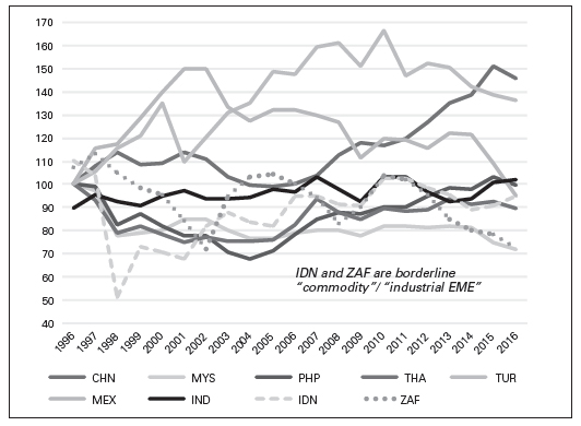
Graph 3 shows the REER performance of “industrial EME”. We index the base year of the data on 1996 as 100, just before the Asian crisis. This implies that the recovery of the Mexican Peso from the peso crisis in December 1994 appears as a great appreciation. Two strongly appreciating countries stand out: Turkey and China. Turkey followed a growth-boom based on current account deficits and building up trade and financial ties with the European Union. China pegged its currency firmly to the USD until 2005, with conspicuous undervaluation of the RMB against the USD and even more against the Euro (which was overvalued against the dollar until 2008). In face of excessive current account surplus, in 2005 the Chinese authorities embarked on a regime change toward managed appreciation against the USD and Euro. Mexico is the only country of this group that followed a real depreciation trend after 2002. The other countries hovered around a more or less horizontal trend of REER.
In contrast, the REER of “commodity EME” tends to be more volatile. Argentina followed a straight downward trend after the 2001 crisis but experienced a significant appreciation after 2009 (due to its relatively high inflation rates)3 3 To account for the well-known underreporting of its official inflation rates in the last years of our sample, Argentina’s REER series represents BIS (2019) data until 2009 and from 2010 onwards it is based on an own calculation. These consider NER data and trade weights from BIS, inflation rates that are reported from the provinces Tucumán, San Luis, Neuquén and Mendoza (simple average), and IFS CPI data of the main trading partners. ; Brazil and Colombia tend to co-move and depreciated heavily until 2003 and are then captured by the commodity boom until 2011 and 2012, respectively. Similarly, Russia’s REER performs in line with the oil price boom until 2013 (as one would predict from Dutch Disease theory), whereas Peru and Chile enjoy surprisingly stable real exchange rates that are similar to the two “industrial EME” India and Indonesia. The benchmark group of commodity-heavy advanced countries, namely Australia, New Zealand and Norway, shows a co-movement with the pattern of the 6 EME (especially with Russia and Colombia), though with a smaller amplitude. The seminal commodity boom is illustrated in Graph 5 with strong differentials between the mining and energy sector and food prices (e.g., the meat price index differs not much from normal inflation).
Most country’s value their currency against the USD, the prime currency on the globe. In Graph 6 we see the nexus between the nominal dollar-rate of an EM-currency in the aggregated “commodity EME” group, the real exchange rate against the USD (RER), the nominal effective exchange rate (NEER) and the REER. The commodity-currencies, grouped together, devalued strongly against the USD until the early 2000s; but their inflation adjusted RER devalued much less. The NEER performs like the NER against the USD, illustrating that the main trade partners co-move strongly against the USD. The bulk of the trade partners is represented by three blocs: the USA, European Union and China (the rest are mainly regional neighbours).
The RER and the REER co-move, but the REER is flatter because different movements within the bloc are neutralised, especially through divergent performance of the USD and Euro. While the REER is relevant for the price competitiveness of companies, the NER against the USD is important for financial flows, given that most financial assets are denominated in this currency. Since nowadays finance tends to have much more influence on exchange rates than trade, the NER to the USD can be considered the main driver for the REER.
Interestingly, the aggregated group performance for the nine “industrial EME” shows a very similar performance (Graph 7). The main difference against the Commodity-EME is that the REER and the other indicators as well are more stable. Again, the grouping hides and neutralises differences within the group (that are visible in the Graphs 3-4).
Looking at the volatility of the REER of the EME (measured by the standard deviation), compared to selected advanced countries, including commodity-prone exporters, we observe a higher volatility for the “commodity EME” with the notable exceptions Chile and Peru, whereas Argentina displays the highest volatility. For the “industrial EME” it is striking that India, Thailand and Malaysia enjoy less volatility than some advanced countries (Graph 8). Using quarterly data, volatility is higher across all countries, but short-term volatility might be less problematic than longer swings. For the EME-15, the mean REER wing-spread (maximum - minimum, as percent of the mean) is 47% over all years and all countries, ranging from only 14% in India to 109% in Argentina. For most EME, the swing-range of EME is much higher than in the USA (29%) and the Euro Area (33%).
With regard to country groups, the descending order of volatility of annual REER is “commodity EME”, advanced commodity producing countries, “industrial EME” and G7 countries - the latter comprises three Euro area countries, which reduces the volatility (Graph 9). It is also important to note that some non-commodity producing advanced countries’ REER is fairly volatile (i.e., Canada and Japan). Finally, Graph 10 shows that the volatility of the NER to the USD is on average higher, and that the ranking amongst countries differs somewhat.
Regarding financial inflows, we use data about annual flows of financial liabilities. We are not sure whether all financial flows can be captured correctly with this indicator. Yet, financial inflows average at 3.4% of GDP, with highest values in Chile and lowest in Indonesia and Thailand (Table 2). The volatility differs across the countries, with a relatively low average of 3.4, compared to an average REER volatility of 11.7. This looks like relatively stable capital inflows but may not capture all the “hot money” flows like those from carry trade.
Finally, it is important to note that the growth performance of our sample countries differs strongly. Graph 11 illustrates the superior performance of most Asian countries, with the exception of Peru and Chile that are in the middle of the ranking. That is to say, “industrial EME” perform significantly better in this respect (except South Africa, Mexico and Thailand). Without the commodity boom, the diverging growth trends would be even bigger.
We summarise tentative answers to the research questions mentioned in the introduction, as far as they can be derived from the descriptive statistical analysis, as follows:
-
Typical sudden stop episodes have been present during the Russian, Brazilian and Argentinian financial crises, in Turkey and Mexico several times, probably amplified by capital flight. Less extreme drops in REER occurred in 2009 and at the beginning of the 2010s.
-
“Commodity” and “industrial” EME groups are heterogeneous. Yet, on average, REER volatility is higher among commodity producers.
-
Russia’s REER trend can be considered as a prototype of classical fossil energy Dutch Disease; the REER of the other “commodity EME” behave similar but less extreme (with the exception of Argentina).
-
There is some co-movement of REER of the commodity EME with commodity-heavy advanced countries like Australia, New Zealand and Norway, but the amplitude of the swings is much bigger. Capital flows could be an amplifier of these swings.
-
Mexico is the only country with a long-trended REER depreciation, China and Turkey tend to appreciate long-term, and the REER of the rest of the countries is relatively flat (with some up - and downswings).
-
Comparing the GDP growth trends with the REER trends indicates that those countries that had relatively stable REER fared much better than those that had a depreciating/appreciating trend. This is true for both “commodity” and “industrial” EME. The notable exception is China.
-
Countries most likely to have depreciation pressure in the future are Argentina, Turkey, Brazil, South Africa and Indonesia (considering their poor S&P rating and macro indicators). The critical point is that expectations on financial crises can easily become self-fulfilling.
REGRESSION ANALYSIS
Methodology
To establish econometrically the main determinants of the above-analysed REER movements in the 15 EME, we use a dynamic panel fixed effects model. We chose a dynamic model on the grounds that it is appropriate to account for the well-known fact that the present value of the REER depends in part on their own lagged value5 5 Some previous studies have used GMM estimators to study the determinants of REER. However, this approach is not viable in our case because the sample has a relatively large T (60 quarters) and small N (15 countries). ; while the incorporation of fixed-effects is important to capture potential unexplained variations at the country level. This approach is broadly in line with studies like Ibarra (2011Ibarra, C.A. (2011). “Capital flows and real exchange rate appreciation in Mexico”. World Development, 39(12): 2080-2090.) and Goda and Torres García (2015Goda, T. & Torres García, A. (2015). “Flujos de capital, recursos naturales y enfermedad holandesa: el caso colombiano”. Ensayos sobre Política Económica, 33(78): 197-206.), which use Autoregressive Distributed-lagged (ARDL) models to determine the REER determinants for Mexico and Colombia, respectively.
The general form of our model is the following:
where t indicates the current period, i is country, ∆ is the difference operator, REER is a real effective exchange rate index, X’ is a set of explanatory variables, a is an unobservable country-specific effect and m is an error term. To account for potential heteroscedasticity and spatial and temporal dependence, we use Driscoll-Kraay standard errors in the regressions (see Hoechle, 2007Hoechle, D. (2007). “Robust standard errors for panel regressions with cross-sectional dependence”. Stata Journal, 7(3): 281-312.).
The period analysed in the regressions spans from 2002Q1-2016Q4. The end of 2016 is the last observation to ensure that the sample is as balanced as possible and considering that at the time of writing the exchange rate regime variable is only available until the end of that year. Meanwhile 2002 has been chosen as starting date because during 1996 and 2001 EME were afflicted by various strong financial crises (as discussed in the third section). The concentration of so many crises in a relatively short time span generates a lot of “noise” that is difficult to control for in an accurate manner. Especially considering that the crises not only had a direct impact on most of the sample countries (Mexico, Asia, Russia, Ecuador, Brazil, Colombia, Argentina and Turkey) but most likely also produced spillover effects.
In accordance with the theoretical and empirical observations from above, and previous studies like Cashin et al. (2004), Nassif et al. (2011Nassif, A., Feijó, C. & Araújo, E. (2011). “The long-term “optimal” exchange rate and the overvaluation trend in emerging countries”. UNCTAD Discussion Paper, No. 206.) and Lartey et al. (2012Lartey, E.K., Mandelman, F.S. & Acosta, P.A. (2012). “Remittances, exchange rate regimes and the Dutch disease: A panel data analysis”. Review of International Economics, 20(2): 377-395.), we consider the commodity terms of trade and real GDP growth rates of each country as potential “structural determinants” of the REER. Real GDP growth rates are intended to proxy the existence of the Harrod-Balassa-Samuelson proposition that rapid productivity growth raises the price of nontradable goods, which in turn appreciates the REER6 6 Please note that Nassif et al. (2011) and Lartey et al. (2012) use real GDP per capita. Given that GDP per capita is not available with quarterly frequency, we choose real GDP as second-best option. . The country-specific commodity terms of trade represent a net export price index for 45 individual commodities that are weighted by the ratio of net exports to total commodity trade. A rise (decline) in commodity prices leads to a rise (decline) in the commodity terms of trade of commodity exporters, whereas it leads to a decline (rise) of the commodity terms of trade of commodity importers (i.e., the “industrial EME” of our sample). To distinguish between potential differential effects that commodity prices have on “commodity” and “industrial” EME, we also employ an interaction term that is derived by multiplying the commodity terms of trade with a dummy that has the value 1 for “commodity EME” and the value 0 for the other countries.
Next to these “structural determinants”, we also consider the following variables: (i) current account balance, (ii) financial account liabilities, (iii) changes in international reserve holdings, (iv) exchange rate regime, (v) VIX, (vi) S&P country ratings (called here “country risk”), and (vii) M3 of OECD countries. In line with the discussions from above, the respective variables are supposed to proxy potential Dutch Disease effects and the impact of current account deficits [(i)], the impact of financial gross inflows due to interest rate differentials, carry trade or investor sentiments [(ii)] - unfortunately we are not aware of publicly available data that allows to consider carry trade directly, nor capital “retrenchment”-, the impact of government exchange rate interventions [(iii))], global risk [(v)], country risk [(vi)], and the impact of monetary policy in core countries [vii)]. To distinguish the peak of the expansionary monetary policies in OECD countries from the other years of the sample period, we create moreover an interaction term that is derived by multiplying the broad money variable with a dummy variable that has the value 1 in all quarters of the years 2008-2010. Finally, we also employ a dummy that accounts for country specific currency crises.
Table 3 summarizes the variables used and their respective data sources, while Table 4 presents the descriptive statistics of these variables. As can be seen, the sample is nearly balanced, with a maximum of 900 observation. The REER index varies between a minimum of 46 and a maximum of 179 index points. However, the variables with the highest standard deviation are the country-specific commodity terms of trade (especially in the case of “commodity EME”) and the OECD broad money index. Furthermore, real GDP growth (from - 16.3% to 16.2%,) the balance of payments variables and the country risk have a considerable range (some countries in some quarters have a “selective default” rating). This shows that not only a lot heterogeneity between countries exist, although all of them are EME, but also that important changes within countries have taken place during the period considered. Finally, it is important to mention that the highest correlation among the variables is 0.52, which indicates that all variables can be included simultaneously in the model without causing multicollinearity issues.
Results
Table 5 shows the regression results. Model (i) considers the “structural forces” of the REER, namely real GDP growth and each country’s commodity terms of trade, and a currency crisis dummy. The results indicate that the cycle of commodity prices plays a significant role for the six commodity producing countries of our sample but has no significant effect on the “industrial EME”. That is to say, increasing (decreasing) commodity prices lead to an appreciation (depreciation) of “commodity EME” currencies, whereas they have no effect on the currencies of “industrial EME”. This finding is in line with the presented hypotheses and the empirical evidence of third section.
The positive and statistically significant coefficient of real GDP growth confirms the existence of the Harrod-Balassa-Samuelson effect, which is reported by various previous studies that analyze the REER determinants of EME (see, e.g., Lartey, 2011Lartey, E.K. (2011). “Financial openness and the Dutch disease”. Review of Development Economics, 15(3): 556-568.; Nassif et al., 2011Nassif, A., Feijó, C. & Araújo, E. (2011). “The long-term “optimal” exchange rate and the overvaluation trend in emerging countries”. UNCTAD Discussion Paper, No. 206.; Ibarra, 2011Ibarra, C.A. (2011). “Capital flows and real exchange rate appreciation in Mexico”. World Development, 39(12): 2080-2090.; Goda & Torres García, 2015Goda, T. & Torres García, A. (2015). “Flujos de capital, recursos naturales y enfermedad holandesa: el caso colombiano”. Ensayos sobre Política Económica, 33(78): 197-206.). However, the statistical significance is not very strong (10%-level). Moreover, the currency crisis dummy is also significant and has the expected negative sign (i.e., a currency crisis leads to a depreciation of EME currencies). It is important to note, that this basic model explains nearly 40% of the REER movements of our sample.
Model (ii) considers the aforementioned “structural forces” and includes additionally balance of payment variables. The previous results stay robust when including these variables. With regard to the other variables, an improvement (deterioration) of the current account balance and financial gross inflows have an appreciating (depreciating) effect, whereas an increase (decrease) in foreign reserves has a depreciating (appreciating) effect. The finding regarding the current account is in line with the Dutch Disease literature, and moreover backs the empirical evidence of third section that substantial current account deficits weaken EME currencies. The result that financial gross inflows appreciate EME currencies is in line with our hypotheses and recent theoretical and empirical evidence (Bresser-Pereira, 2009Bresser-Pereira, L.C. (2009): “The tendency to the overvaluation of the exchange rate”. In Bresser-Pereira, L.C. (ed.): Globalization and Competition. Cambridge: Cambridge University Press, 125-147.; Cardarelli et al., 2010; Ibarra, 2011Ibarra, C.A. (2011). “Capital flows and real exchange rate appreciation in Mexico”. World Development, 39(12): 2080-2090.; Goda & Torres García, 2015Goda, T. & Torres García, A. (2015). “Flujos de capital, recursos naturales y enfermedad holandesa: el caso colombiano”. Ensayos sobre Política Económica, 33(78): 197-206.; Botta, 2017Botta, A. (2017). “Dutch Disease-cum-financialization booms and external balance cycles in developing countries”. Brazilian Journal of Political Economy, 37(3): 459-477.). The negative sign of the foreign reserve variable suggests that the interventions of EME Central Banks to avoid more substantial appreciations (depreciations) were at least partially successful.
Finally, Model (iii) controls for the effect of financial openness, global risk, country risk and the amount of broad money that is in circulation in OECD countries. In this specification, the variables real growth and “commodity EME” terms of trade become more significant. As expected, we also find that an increase (decrease) in country risk leads to a REER depreciation (appreciation). Interestingly, global risk and the broad money stock of OECD countries have no statistically significant effect on EME currencies. However, when only considering the period of the global recession and the peak of the accommodating monetary policies in OECD countries (2008 to 2010) the increase in broad money had the expected appreciating effect. This result is in line with previous findings that the monetary policies of core countries has some spillover effects on peripheral countries (Aizenman et al., 2016Aizenman, J., Chinn, M. & Ito, H. (2016). “Monetary policy spillovers and the trilemma in the new normal: periphery country sensitivity to core country conditions”. Journal of International Money and Finance, 68: 298-330.).
CONCLUSIONS
The aim of this paper was to study the determination of REER in 15 EME. The results of this exercise indicate that EME are heterogenous, especially “commodity” and “industrial” EME. REER volatility tends to be higher among the former. Yet, REER volatility between emerging and advanced countries does not differ much, apart from a few EME. Countries that had a more stable REER fared better than those that had a depreciating or appreciating trend (with the notable exception of China). As theoretically expected, commodity terms of trade are an important structural driver of REER movements in “commodity EME”. However, the experiences of countries that are dependent on mining and energy commodities tend to be somewhat different than that of agriculture-dependent countries.
Moreover, it is crucial to consider financial inflows when studying EME REER movements. Unfortunately, it is difficult to control for important factors like carry-trade. Better data and more research on the topic is needed. The results also confirm the existence of the Harrod-Balassa-Samuelson effect, and the partial success of countries that intervene in the FX-market to avoid more substantial appreciations (depreciations). Furthermore, we find that lower country risk and, at least in some periods, growing broad money in OECD countries has led to REER appreciations in EME.
In line with the propositions of “New Developmentalism”, the data also suggests that EME with a relatively stable REER and current account surpluses fared much better in terms of overall macroeconomic indicators than those that had not. However, the examples of China and Mexico show that for upper-middle countries the concept of competitive “industrial REER” needs further investigation (China has a growing manufacturing sector and a REER with an appreciating trend, whereas Mexico has a depreciating trend and a declining manufacturing sector). Several of the better performing EME were able to demobilise their monetary policy rates without endangering their currency stability (sometimes thanks to capital controls). Finally, the problem of high interest rates in EME needs more attention in future research. With a permanent GDP growth rate far below the interest rate, credit markets tend to be a big barrier to growth.
REFERENCES
- Adrian, T., Etula, E. & Shin, H.S (2015). “Risk Appetite and Exchange Rates”. Federal Reserves Bank of New York Staff Reports, No. 361.
- Aizenman, J., Chinn, M. & Ito, H. (2016). “Monetary policy spillovers and the trilemma in the new normal: periphery country sensitivity to core country conditions”. Journal of International Money and Finance, 68: 298-330.
- Andrade, R.P. & Prates, D.M. (2013). “Exchange rate dynamics in a peripheral monetary economy: a Keynesian perspective”. Journal of Post-Keynesian Economics, 35(3): 399-416,
- BIS (2016): Triannual Central Bank Survey. Foreign Exchange Turnover in April 2016. Basle: Bank of International Settlement.
- Blanchard, O., Adler, G. & de Carvalho Filho, I. (2015). “Can foreign exchange intervention stem exchange rate pressures from global capital flow shocks?”. IMF Working Paper, No. 15/159.
- Botta, A. (2017). “Dutch Disease-cum-financialization booms and external balance cycles in developing countries”. Brazilian Journal of Political Economy, 37(3): 459-477.
- Bresser-Pereira, L.C. (2009): “The tendency to the overvaluation of the exchange rate”. In Bresser-Pereira, L.C. (ed.): Globalization and Competition. Cambridge: Cambridge University Press, 125-147.
- Bresser-Pereira, L.C. (2019). “From classical developmentalism and post-Keynesian macroeconomics to new developmentalism”. Brazilian Journal of Political Economy, 39(2): 187-210.
- Chen, Q., Filardo, A., He, D. & Zhu, F. (2015). “Financial crisis, us unconventional monetary policy and international spillovers”. IMF Working Paper, No. 15/85.
- Deutsche Bundesbank (2017). „Globale Liquidität, Devisenreserven und Wechselkurse von Schwellenländern“. Deutsche Bundesbank Monatsbericht, Oktober: 13-27.
- Forbes, K. & Warnock, F. (2012), “Capital flow waves: surges, stops, flight and retrenchment”. Journal of International Economics, 88(2): 235-251.
- Fratzscher, M., Gloede, O., Menkhoff, L., Sarno, L. & Stöhr, T. (2017). “When is foreign exchange intervention effective? Evidence from 33 countries”. DIW Discussion Paper, No. 1518 (revised).
- Goda, T. & Priewe, J. (2019). “Determinants of real exchange rate movements in 15 emerging market economies”. CIEF Working Paper, No. 19-13.
- Goda, T. & Torres García, A. (2015). “Flujos de capital, recursos naturales y enfermedad holandesa: el caso colombiano”. Ensayos sobre Política Económica, 33(78): 197-206.
- Hoechle, D. (2007). “Robust standard errors for panel regressions with cross-sectional dependence”. Stata Journal, 7(3): 281-312.
- Ibarra, C.A. (2011). “Capital flows and real exchange rate appreciation in Mexico”. World Development, 39(12): 2080-2090.
- IMF (2019). World Economic Outlook Database (July). https://www.imf.org/external/pubs/ft/weo/2019/01/weodata/index.aspx
» https://www.imf.org/external/pubs/ft/weo/2019/01/weodata/index.aspx - Isard, P. (2008). Exchange Rate Economics. Cambridge: Cambridge University Press .
- Kaltenbrunner, A. (2015). “A post Keynesian framework of exchange rate determination: a Minskyan approach”. Journal of Post Keynesian Economics, 38(3): 426-448.
- Lartey, E.K. (2011). “Financial openness and the Dutch disease”. Review of Development Economics, 15(3): 556-568.
- Lartey, E.K., Mandelman, F.S. & Acosta, P.A. (2012). “Remittances, exchange rate regimes and the Dutch disease: A panel data analysis”. Review of International Economics, 20(2): 377-395.
- Menkhoff, L. (2013). “Foreign exchange intervention in emerging markets: A survey of empirical studies”. World Economy, 36: 1187-1208.
- Minsky, H. (1986). Stabilizing an Unstable Economy. New York: McGraw-Hill.
- Naceur, S.B., Bakardzhieva, D. & Kamar, B. (2012). “Disaggregated capital flows and developing countries’ competitiveness”. World Development, 40(2): 223-237.
- Nassif, A., Feijó, C. & Araújo, E. (2011). “The long-term “optimal” exchange rate and the overvaluation trend in emerging countries”. UNCTAD Discussion Paper, No. 206.
- Pilbeam, K. (2013). International Finance. Houndsmills, New York: Palgrave Macmillan.
- Ramos, R.A. & Prates, D.M. (2018). “The Post-Keynesian view on exchange rates: towards the consolidation of the different contributions in the ABM and SFC frameworks”. UNICAMP Texto para Discussão, No. 352.
- Rey, H. (2015, revised 2018). “Dilemma and Not Trilemma: The Global Financial Cycle and Monetary Policy Independence”. NBER Working Paper, No. 21162.
- Venables, A.J. (2016). “Using natural resources for development. Why has it proven so difficult?” Journal of Economic Perspectives, 30(1): 161-184.
-
1
Please see Goda & Priewe (2019Goda, T. & Priewe, J. (2019). “Determinants of real exchange rate movements in 15 emerging market economies”. CIEF Working Paper, No. 19-13.) for a more detailed description of the main tenets of “New Developmentalism” regarding exchange rates issues, and an extended overview on the existing literature regarding exchange rates in EME.
-
2
EMP can be measured (among other indicators) by the change rate of nominal EM-exchange-rates (foreign currency per local currency unit) and by the change of central banks’ currency reserves.
-
3
To account for the well-known underreporting of its official inflation rates in the last years of our sample, Argentina’s REER series represents BIS (2019) data until 2009 and from 2010 onwards it is based on an own calculation. These consider NER data and trade weights from BIS, inflation rates that are reported from the provinces Tucumán, San Luis, Neuquén and Mendoza (simple average), and IFS CPI data of the main trading partners.
-
4
For the calculation of Argentina’s RER, we use here inflation rates for Argentina by the IMF (2019). For a few years, the IMF provides only GDP deflators, not CPI. In these cases, we use the GDP deflator instead of CPI.
-
5
Some previous studies have used GMM estimators to study the determinants of REER. However, this approach is not viable in our case because the sample has a relatively large T (60 quarters) and small N (15 countries).
-
6
Please note that Nassif et al. (2011Nassif, A., Feijó, C. & Araújo, E. (2011). “The long-term “optimal” exchange rate and the overvaluation trend in emerging countries”. UNCTAD Discussion Paper, No. 206.) and Lartey et al. (2012Lartey, E.K., Mandelman, F.S. & Acosta, P.A. (2012). “Remittances, exchange rate regimes and the Dutch disease: A panel data analysis”. Review of International Economics, 20(2): 377-395.) use real GDP per capita. Given that GDP per capita is not available with quarterly frequency, we choose real GDP as second-best option.
-
7
JEL Classification: F6; F31; F41; O11; O57; P52.
-
***
We thank Cristhian Larrahondo for his excellent research assistance, and the participants of the 4th FGV Workshop on New Developmentalism for their helpful comments.
Data availability
Data citations
IMF (2019). World Economic Outlook Database (July). https://www.imf.org/external/pubs/ft/weo/2019/01/weodata/index.aspx
Publication Dates
-
Publication in this collection
17 Apr 2020 -
Date of issue
Apr-Jun 2020
History
-
Received
19 July 2019 -
Accepted
01 Aug 2019

 Source: WDI (2019).
 Source: WDI (2019).
 Source:
  Source:
  Source:
 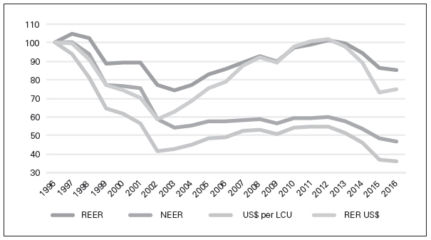 Source:
  Source:
  Source:
  Source:
 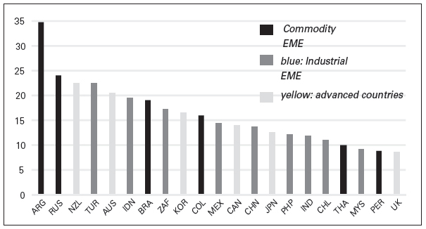 Source: BIS, own calculations.
 Source: WDI (2019)