Welfare Consequences of Persistent Climate Prediction Errors on Insurance Markets against Natural Hazards

Abstract

This paper studies the welfare consequences of the friction between two groups, those with and those without rational expectations, in an incomplete insurance market. We validate this friction empirically and test the existence of additional heterogeneity in the probability of belonging to the group which makes persistent mistakes on the anticipation of climate events using econometric models. The econometric models further suggest that the probability of belonging to this group varies significantly by sociodemographic attributes of respondents and by the geophysical attributes of their places of residence. Based on this evidence, we develop a two-period model of private insurance under uncertainty with endogenous prices. By including a central planner providing a technology for access to accurate information, our example illustrates that public intervention (via taxation) would only be feasible if public expenditure in the provision of this technology did not exceed 9.188% of the aggregate income earned by agents with inaccurate expectations.

Keywords
Climate uncertainty; Risk aversion; Insurance Contracts; River flooding; Subjective probability

Resumo

Este artigo estuda as consequências da fricção entre dois grupos de agentes econômicos, com e sem expectativas racionais, sobre o bem-estar econômico em um mercado de seguro incompleto. Utilizando modelagem econométrica, validamos essa fricção empiricamente e testamos a existência de heterogeneidade adicional na probabilidade de pertencimento ao grupo que comete erros persistentes sobre a antecipação de eventos climáticos futuros.

Os modelos econométricos sugerem adicionalmente que essa probabilidade varia significativamente por atributos sociodemográficos dos indivíduos e por atributos geofísicos de seus locais de residência. Com base nessas evidências, desenvolvemos um modelo de seguro privado de dois períodos sob incerteza com preços endógenos. Ao incluir um planejador central, o qual provê uma tecnologia para obtenção de informação precisa, nosso exemplo ilustra que a intervenção pública (via tributação) somente seria factível se o gasto público na provisão dessa tecnologia não excedesse 9.188% da renda agregada gerada pelos agentes com expectativas adaptativas.

Palavras-Chave
Incerteza climática; Aversão ao risco; Contratos de Seguro; Inundação fluvial; Probabilidade subjetiva

1. Introduction

Climate change has altered agents' ability to anticipate the future occurrence of events with high degree of accuracy (Parker 2010; Dasgupta 2008; Regan et al. 2005). This subjective anticipation may be inaccurate, leading to Pareto inferior choices when compared to a situation where agents have rational expectations (Savage 1951; Yohe et al. 2004; Prato 2008). In this case, market equilibrium and demand for insurance are better understood using models that explicitly incorporate agents' heterogeneity in the degree of prediction accuracy.

Until now most models used in insurance economics with heterogeneous agents have tried to explain market allocation of insurance using differential information. These models' results focus on issues related to adverse selection and moral hazard (Mirlees 1971; Atkison and Stiglitz 1972; Laffont and Tirole 1987). These types of heterogeneity, as used in Crocker and Snow's (1985) and Picard's (1987) models, consider differences in the consumer's information structure, but not in their subjective probabilities directly. In this case, market failures arise due to a supply shortage caused by negative profit or demand shortage as a consequence of excessively high prices.

In markets where contractual insurance is not available, moral hazard and adverse selection are of little relevance for market allocation. Many studies that analyze the trade-off between the demand for insurance, self-insurance, and self-protection¹ reinforce this argument, by either looking at agents' reservation price or by taking insurance price as actuarily fair (Ehrlich and Becker 1972, Dionne and Eeckhoudt 1985, Lakdawalla and Zanjani 2005, Snow 2011, Alary et al. 2013).

Most of the previous models look at the effect of information asymmetry on the demand for insurance using a representative agent. By assuming homogeneity in agents' preferences, they ignore the influence of this effect on equilibrium prices, which would be the most interesting economic problem to be studied. The scarcity of studies on insurance models with endogenous prices is mainly explained by the difficulty in obtaining the price solutions.²

Another important issue to be considered in insurance models is the role played by a central planner to attenuate the effect of information asymmetry in market allocation (Caillaud et al. 1988). Arnott and Stiglitz (1990), for instance, show that taxation and subsidization policies providing incentives to avoid and reduce losses are not effective in markets in which moral hazard arises from information asymmetry. When public intervention is used to solve the insurability problem using increased taxation (as discussed by Mangan 1995), risk can increase in the long run. Additional pressure on the government to increase coverage, keeping the risk premiums unaltered, is also a likely moral hazard consequence of taxation (Dionne et al. 2000). This situation is similar to a market with mandatory insurance acquisition, with premiums partially financed by the government. However, we show that it is still possible to implement a public technology supported by a tax levy to correct information asymmetry represented by errors in the probabilities on natural events. Since intervention affects information on selected groups instead of on insurance directly, the problem of moral hazard is irrelevant and can be ignored.

This paper has four main goals. First, we study the welfare consequences of the friction between two groups, those with and those without rational expectations, in an incomplete insurance market. We validate this friction by seeking empirical evidence of persistent errors in a subsample of individuals regarding their perception of change in local climate parameters. Second, we test the existence of additional heterogeneity in the probability of belonging to the group which makes persistent mistakes on the anticipation of climate events using econometric models. Third, we develop a two-period model of private insurance under uncertainty with endogenous prices³ to explain how the coexistence of these groups may deviate market prices from the fundamentals, leading to a reduction in social welfare in the long run. Our proposed model differs from that of Rotschild and Stiglitz (1976) by considering heterogeneous beliefs and income taxation to correct market failures (information asymmetry). The tax burden⁴ is employed to finance a public technology that provides accurate information to those agents making persistent mistakes.⁵ The levy only on agents without rational expectations is a way to avoid moral hazard behavior among those with rational expectation (Mirlees 1971; Atkison and Stiglitz 1972). Finally, we solve the proposed model algebraically with a closed form solution and simulate the taxation threshold as a proportion of the agents' income that Pareto improves any market allocation without government intervention.

Based on novel survey data, we identified the existence of a group of individuals making persistent errors in the anticipation of climate events. Our econometric models further suggest that the probability of belonging to this group varies significantly by sociodemographic attributes of respondents and by the geophysical attributes of their places of residence. This empirical finding of heterogeneity within and between groups helps explain why there is no market supply of information on natural events.

The absence of firms providing this type of information occurs because price discrimination via product differentiation is economically unfeasible in private markets. Therefore, we propose a theoretical model with heterogeneous agents and taxation to finance a public technology providing information on natural events.

Results from our insurance model with incomplete markets show that the group with accurate expectations price the insurance as the economic fundamentals (Rotschild and Stiglitz 1976), while agents with inaccurate expectations distort insurance prices in the long run. The closed form solution suggests that agents making persistent mistakes in the process of anticipation of climate events are not driven out from the market, as in Blume and Easley (2006). By including a central planner providing a technology for access to accurate information, our example illustrates that public intervention (via taxation) would only be feasible if public expenditure in the provision of this technology did not exceed⁶ 9.188% of the aggregate income earned by agents with inaccurate expectations. This threshold is computed based on a relative measure of social welfare that is robust to scale transformations.

2. Empirical Evidence on Agents' Heterogeneity

2.1 Climate Data

To understand the evolution of objective climate parameters we use climate data (precipitation and temperature) from all the six meteorological stations located in the municipality of Governador Valadares, Brazil. Data were provided by the Center for Weather Forecast and Climate Studies (CPTEC), at the Brazilian Institute for Spatial Research (INPE), and by the Brazilian Institute of Meteorology (INMET). Different stations were pooled together, since not all had valid information for the same time window. Station data pooling allowed us to recreate the time series of climate information after some forecasting and data smoothing.

Some decision rules were taken to interpolate the data: (1) when there was only one piece of information available for a climate parameter (from 1 station only), this information was used to create the time series; (2) when more than one station provided data for the same parameter at the same date, the average of these measures were used. The spatial location of meteorological stations shows no geophysical barrier⁷ (such as the Ibituruna Peak in the outskirts of the city), which could affect climate parameters through heat island or humidity alteration effects. Thus, simple average for the parameters could be used with no significant estimation bias (Ashraf, Loftis and Hubbard 1997).

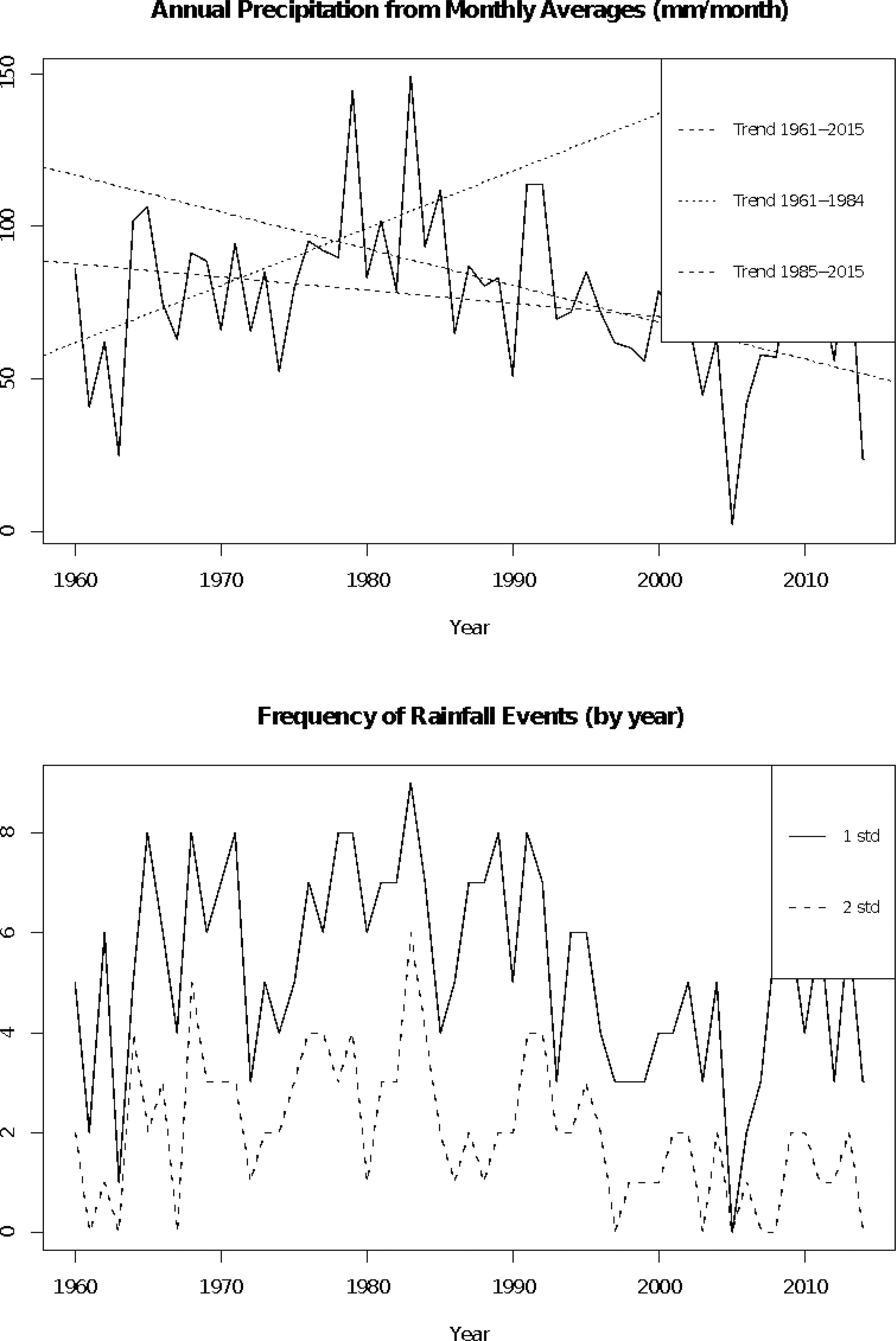
Despite many climate parameters available in the climate data, we selected only temperature and precipitation for this study. These data were measured on a daily basis, with different temporal gaps per station. The decision rules previously described allowed us to recreate historical climate series data from 1960 to 2014 for precipitation. Daily data were transformed into monthly averages. Precipitation data were classified by: (a) intensity and (b) frequency (Figure 1). Precipitation intensity was measured as the annual average of monthly precipitation (in mm/month). Precipitation frequency was measured as the number of monthly precipitation events higher than 1 or 2 standard deviations of the annual average.⁸ Figure (1) suggests an increase in rainfall intensity and frequency from 1960 to 1983, followed by decreased parameters from 1983 to 2014.

Figure 1
Average Monthly Precipitation Intensity and Frequency - Governador Valadares, Brazil - 1960 to 2014

Since we compare perceptions of local climate change with objective climate data to proxy the agents' prediction errors, we may incur the risk of perceptions related to long periods backward being contaminated by memory bias. Thus, assuming that memory bias is small from 1990 onward (only 25 years of contrasts), trends in climate parameters look different. Figure (1) reveals that between the late 1990s and 2005 rainfall frequency and intensity declined, with the opposite trend being observed for the more recent period (2005 to 2014). This recent trend mirrors the trend observed from 1960 to 1983. Our analyses then were based on three time windows: full memory (1960-1983 / 1984-2004 / 2005-2015), long-term memory (1960-1983 / 1984-2014) and short-term memory (1990-2004 / 2005-2014). The empirical results using these three time windows suggest different degrees of precision in the anticipation of the true probabilities. This justifies the analysis of a spectrum of errors in the probabilities of our numerical example (described later in the text).

Historical data on temperature is less reliable than data on precipitation, with more missing records over the period considered here. Daily data from 1960 to 2015 were transformed into monthly averages. After transformation, several months had missing information for select years. To smooth the time series, we used a structural model, as described in Harvey and Todd (1983). The main advantage of the structural model for time series is the use of the series in level (instead of the differenced series, such as the traditional ARIMA models). This feature avoids using less information due to differencing, especially when the gaps are considerably large and located in different points over the time range. We can describe the model as follows.

Let 𝑦_t be an observed variable. The basic structural model has the form:

${\mathit{y}}_{\mathit{t}}={\mathit{\mu }}_{\mathit{t}}+{\mathit{\gamma }}_{\mathit{t}}+{\mathit{\varepsilon }}_{\mathit{t}},\mathit{where}\mathit{t}=1,\cdots ,\mathit{T}$

where 𝜇_t, 𝑦_t and 𝜖_t represent the trend, seasonality, and error terms, respectively. The generating process for the trend component is defined as:

${\mathit{\mu }}_{\mathit{t}}={\mathit{\mu }}_{\mathit{t}-1}+{\mathit{\beta }}_{\mathit{t}-1}+{\mathit{\eta }}_{\mathit{t}},\mathit{where}{\mathit{\beta }}_{\mathit{t}}={\mathit{\beta }}_{\mathit{t}-1}+{\mathit{ç}}_{\mathit{t}},\mathit{for}\mathit{t}=1,\cdots ,\mathit{T}$

where 𝜂_t and 𝜍_t are normally distributed white noise independent processes, with mean 0 and variance 𝜎_𝜂² and 𝜎_𝜍². A key feature of this model is that it is a local approximation of a linear trend. The level and the slope change smoothly according to a random walk mechanism. The generating process for the seasonal component is given by:

${\mathit{\gamma }}_{\mathit{t}}=\sum _{\mathit{j}=1}^{\mathit{s}-1}{\mathit{\gamma }}_{\mathit{t}-\mathit{j}}+{\mathit{\omega }}_{\mathit{t}},\mathit{where}\mathit{t}=1,\cdots ,\mathit{T}$

where ${\mathit{\omega }}_{\mathit{t}}\sim \mathit{NID}\left(0,{\mathit{\sigma }}_{\mathit{\omega }}^2\right)$ and is the number of seasons. The seasonal pattern evolves smoothly by a mechanism that assures the sum of seasonal components over time, in any consecutive time periods, be 0 (expected value) with constant variance over time. The disturbances 𝜂_t, 𝜍_t and 𝜔_t are cross-independent and the error component is a normally distributed white noise process, that is, ${\mathit{\varepsilon }}_{\mathit{t}}\sim \mathit{NID}\left(0,{\mathit{\sigma }}^2\right)$.

From the 56-year window (1960 to 2015) we obtained reliable data (complete or with high levels of prediction accuracy) for the following subperiods: 1960-1978, 1995-2004, 2007, and 2010-2015. The gaps between these subperiods were smoothed by applying the structural model for time series on the temperature data.⁹ Treated temperature data series shows a tendency of local cooling until 1980 (and a new cooling period between 1995 and 2005), followed by average temperature increase after the mid-2000s (Figure 2).

Figure 2
Average Yearly Temperature - Governador Valadares, Brazil - 1960 to 2014

These local climate data were used as an objective criterion for comparison with individuals' perception of local climate change for Governador Valadares. Perceptions were derived from survey data collected in the region. These two sources of climate data combined proxy parameters from our theoretical model (described further in the text), represented by the objective (𝜋^𝜄_S) and subjective (𝜋^𝑖_S) probabilities, respectively. These contrasts were used within an econometric framework to seek evidence

of a subgroup of sampled individuals making persistent mistakes in the anticipation of occurrence of natural events.

2.2. Survey Data

Our theoretical model of choice under climate uncertainty assumes subjective beliefs regarding the probability of future event occurrence. An interesting aspect of agents' adaptive behavior is to understand the sociodemographic profile that explains the observed variability on these subjective priors, which lead some agents to make persistent mistakes when objective and subjective patterns of change in local climate parameters differ. Furthermore, understanding which population subgroups are more likely to perceive a divergent climate trend may help tailor better risk management strategies at the local level.

To seek empirical evidence of this type of heterogeneity, we make use of novel survey data collected in Governador Valadares, Brazil. The survey data used here come from a pioneering research project in Brazil addressing environmental attitude, awareness, and behavior at the local level, with detailed questions on climate change perception and adaptive measures under risk of flooding. Data are part of the research project entitled "Migration, Vulnerability, and Environmental Change in the Rio Doce Valley", funded by the Minas Gerais Research Foundation (FAPEMIG Grant CSA-APQ-00244-12, FAPEMIG Grant CSA-PPM-00305-14, and FAPEMIG Grant CSA-APQ-01553-16), the Brazilian Research Council (CNPq Grant 4837/2012-7, CNPq Grant 472252/2014-3, CNPq Grant 431872/2016-3, and CNPq Grant 314392/2018-1), and the Brazilian Network on Global Climate Change Research (FINEP/ Rede CLIMA Grant Number 01.13.0353-00). The project was approved by the Research Ethics Committee at the Universidade Federal de Minas Gerais (Protocol CAAE 12650413.0.0000.5149).

Face-to-face interviews were conducted in the urban area of Governador Valadares between 2014 and 2015, based on a questionnaire¹⁰ successfully applied in other countries (Terpstra and Lindell 2013) and for other hazards (Grothmann and Reusswig 2006; Kievik and Gutteling 2011; Zaalberg et al. 2009). The survey was based on a multi-stage sampling design. The first stage used clusters of neighborhoods, with clustering based on geographic proximity and socioeconomic status of the neighborhood. Within each cluster, sample was stratified by sex and age groups, and within each stratum households were randomly selected. A minimum sample size was estimated of 1,069 households, based on a significance level of 5% and a tolerance of 3% for sample proportions. Variance estimate was 0.25, yielding the most conservative minimum sample size (Groves et al. 2011). Because of additional budget resources granted, sample size was increased to 1,226 households.

2.3. Comparative Analysis

In order to compare the local climate parameters (temperature and precipitation) with their population perception we used the following items available in the survey questionnaire: (a) temperature: "In your opinion, since you started living in Governador Valadares, the city is: (1) as hot as in the past, (2) hotter than in the past, (3) cooler than in the past, (4) I don't know"; (b) precipitation: "In your opinion, since you started living in Governador Valadares, it rains: (1) as often and with same intensity, (2) more often, but with same intensity, (3) more often and more intensively, (4) less often, but with same intensity, (5) less often and less intensively, (6) more often, but with less intensity, (7) less often, but with same intensity, (8) it is impossible to know, (9) did not answer.

Based on these two questions and the climate data, we created a dummy variable for each climate parameter: (1) Perception and climate data differ (mismatch); (0) Perception and climate data converge (no mismatch). We ground our descriptive analysis on two different sets of dependent variables: (1) perception of any change (on both temperature and precipitation from survey data), and (2) perception mismatch (survey versus climate data). For the first set, we split the analysis into rain pattern and temperature change perception. The first discriminated the following rain pattern categories: more frequent, less frequent, more intense, less intense, and missing information. The second discriminated the following temperature pattern categories: same, hotter, cooler, and missing information. The second set comprises descriptive association between covariates and the dependent variable (mismatch) for the three time windows considered: full memory, long memory, and short memory.

We then moved to a regression-based association, with two main models: (1) model of perceived change (survey data only), and (2) models of mismatch (survey versus climate data). Since questions on perception of temperature and precipitation change were answered by the same respondent, they are probably correlated on unobserved determinants. Because of this potential conditional correlation, we model the two dummy variables within a bivariate probit system of equations. To estimate sociodemographic patterns related to the contrasts (convergence and divergence between perception and measurement), we used the following covariates: age, age variance of household members, sex, individual income, education, time of residence, network distance to the Doce River, if the household is located in a flood-prone area, if any household member was ever hit by a river flood in the city, and if there is serious lack of green areas in the household surroundings. The general econometric framework for the bivariate probit system of two equations can be summarized as:

$\begin{array}{c}{\mathit{y}}_{\mathit{P}}^{*}={\mathit{X}}_{\mathit{P}}{\mathit{\beta }}_{\mathit{P}}+{\mathit{\varepsilon }}_{\mathit{P}},\mathit{if}{\mathit{y}}_{\mathit{P}}^{*}>0,0\mathit{otherwise}{\mathit{y}}_{\mathit{T}}^{*}={\mathit{X}}_{\mathit{T}}{\mathit{\beta }}_{\mathit{T}}+{\mathit{\varepsilon }}_{\mathit{T}},\mathit{if}{\mathit{y}}_{\mathit{T}}^{*}>0,\\ 0\mathit{otherwise}\left({\mathit{\varepsilon }}_{\mathit{P}}{\mathit{\varepsilon }}_{\mathit{T}}\left|{\mathit{X}}_{\mathit{P}},{\mathit{X}}_{\mathit{T}}\right.\right)\sim \mathit{N}\left[\left(00\right),\left(1\mathit{\rho }\mathit{\rho }1\right)\right]\end{array}$

where 𝑦_P^* stands for a n × 1 vector of individual propensity¹¹ to perceive any change in the local precipitation pattern (or the propensity to mismatch perception with objective change from precipitation data); 𝑋_P is a 𝑛 × 𝑣 matrix of covariates¹² affecting the propensity; 𝛽_P is a 𝑣 × 1 vector of covariates effects on 𝑦_P^*, and 𝜖_P is the 𝑛 × 1 vector of disturbances. The matrices (or vectors) 𝑦_T^*, 𝑋_T, 𝛽_T and 𝜖_T are the analogous for the temperature model.

The model was estimated by maximum likelihood. Although the correlation parameter, ρ, is not directly estimated, it can be obtained by simple manipulation of the estimated parameter, atanh(ρ), also known as τ, given as:

$\mathit{\tau }=\mathit{a}\mathit{tanh}\left(\mathit{\rho }\right)=\frac{1}{2}\mathit{ln}\mathit{ln}\left(\frac{1+\mathit{\rho }}{1-\mathit{\rho }}\right)$

that is,

$\mathit{\rho }=\left[\mathit{exp}\mathit{exp}\left(2\mathit{\tau }\right)-1\right]/\left[\mathit{exp}\mathit{exp}\left(2\mathit{\tau }\right)+1\right]$

The ρ parameter, constrained to the interval [-1,1], represents the tetrachoric conditional correlation for two dummy variables, that is, the conditional correlation on unobservables. A Likelihood Ratio test (LR) can be performed for the non-zero ρ. The LR statistic can be obtained by comparing the bivariate solution for the maximum likelihood and the sum of univariate maximum likelihood solutions for each probit error, as follows:

${\mathit{\lambda }}_{\mathit{LR}}=2\left[\mathit{ln}{\mathit{L}}_{\mathit{BIVARIATE}}-\left(\mathit{ln}{\mathit{L}}_1+\mathit{ln}{\mathit{L}}_2\right)\right]\sim {\mathit{\chi }}^2\left(1\mathit{df}\right)$

If the parameter ρ is significantly different from zero, the coefficients' variance will be more efficient if estimated by the bivariate probit model.

2.4. Descriptive Results

Our survey data (Table 1) showed that 65.8% of respondents identify some change in the local temperature since they started living in Governador Valadares (58.3% think the temperature increased and 7.5% believe that the city is cooler than in the past). Only 26.7% perceived no change in local temperature over those years. Less than 8% of respondents did not answer the question.

Table 1
Descriptive analysis of sociodemographic attributes and its relation to perception of change in local climate parameters - Governador Valadares, Brazil, 2014/2015

Covariates	Rain Pattern
	More	Less	More	Less	Doesn't
	Frequent	Frequent	Intense	Intense	Know
Male	39.7	45.7	55.0	43.7	46.7
Age	38.9	41.0	38.5	40.9	34.8
Std. Dev. of age in household	15.0	15.6	15.0	15.5	12.4
Incomplete high school	34.5	31.3	27.5	33.1	16.7
Incomplete college	44.8	47.0	50.3	46.8	51.7
Complete college	20.7	21.7	22.1	20.0	31.7
Near distance to river (km)	1.7	1.4	1.6	1.4	1.2
Household in flood-prone area	22.4	19.8	20.8	19.2	25.0
Any in household ever hit by flood	29.3	27.9	28.9	24.4	1.7
Sample (%)	6.8	82.3	16.9	57.0	5.3
Covariates	Temperature
	Same	Hotter	Cooler	Doesn't Know
Male	46.4	44.1	48.1	48.8
Age	43.0	40.4	42.6	36.8
Std. Dev. of age in household	14.7	15.6	16.2	12.6
Incomplete high school	33.6	30.6	33.8	13.8
Incomplete college	44.2	47.7	40.3	60.0
Complete college	22.3	21.7	26.0	26.3
Near distance to river (km)	1.4	1.4	1.7	1.3
Household in flood-prone area	24.5	15.8	31.2	33.8
Any in household ever hit by flood	29.6	25.5	23.4	7.6
Sample (%)	26.7	58.3	7.5	7.5

Source: Authors' estimation based on Survey Data (Governador Valadares, 2014/2015).

The lower panel of Table 1 shows that sociodemographic patterns differ depending on how temperature change is perceived. On average, women, younger residents, those living longer in the city, the less educated, and those living closer to the Doce River, but out of the flood-prone areas, are more likely to perceive an increase in local temperature over their time of residence (compared to temperature cooling). Younger residents with a larger within-household age variance, more recent residents, those living further from the Doce River, and those not having been directly affected by the river floods are most likely to perceive any change (against no perception of change).

Descriptive data on perception of precipitation change also reveal interesting patterns: age is not very relevant, although those perceiving rainfall as more frequent and intense are slightly younger.¹³ While women perceive more frequent rainfall, men are more likely to perceive increase in rainfall intensity over their time of residence. Women, however, are more likely to perceive less frequent and intense rain than men over time. Time of residence seems to be linked to increased likelihood of temperature perception mismatch, regardless of the time window. For precipitation, however, newer immigrants are less likely to have a divergent perception for the shorter period, the opposite holding for the long time window. This is likely to reflect a mix of acclimatization and endogeneity between perception and place attachment (Grothmann and Patt 2005).

Women and those living in less educated households are less likely to perceive more intensive rain patterns; these patterns may reflect both vulnerability and exposure to worse locational conditions. Those living farther away from the Doce River, but within the flood-prone area, and those ever directly affected by a river flood in town are more likely to perceive increased intensity and frequency. These patterns may be explained by two quite different reasons: while those far from the river may seek environmental cues on change in the water level while raining, those directly affected by the experience with an extreme event may trigger what is known as the magnified perception of risk (Pidgeon, Kasperson and Slovic 2003). Those that are less likely to have noticed any change in precipitation patterns are quite younger, living in households with a smaller age variance of residents, more likely to reside in a more educated migrant household, located close to the Doce River, within flood-prone areas and with very low probability of ever having been hit by a river flood in town.

Although interesting by itself, the comparison of sociodemographic groups by type of perceived change is less likely to provide a more solid clue on agents' heterogeneity regarding the probability of perception mismatch. A better way to look at it descriptively is to analyze the perception mismatch directly. Table 2 presents bivariate summary measures for the three time windows previously discussed. If we look at persistent relations, regardless of the time window, we find that more educated men and those with some experience with floods from the Doce River are more likely to perceive a different trend in local climate parameters than what is suggested by the meteorological data. Age is only important for the full and long memory time windows, as older people are more likely to mismatch their perceptions with climate data. As anticipated, memory bias seems to be reduced for the short memory time window. These patterns hold for both precipitation and temperature.

Table 2
Descriptive analysis of sociodemographic attributes and its relation to divergence between perceived and objective change in local climate parameters - Governador Valadares, Brazil, 2014/2015.

Covariates	Rain Pattern		Temperature
	Mismatch	No Mismatch	Mismatch	No Mismatch
	Full Memory
Male	45.9	42.5	46.2	39.4
Age	43.9	29.7	41.0	39.7
Std. Dev. of age in household	15.3	16.1	15.6	14.4
Years continuously living in GV	30.4	20.4	30.4	15.8
Incomplete high school	31.9	30.6	31.8	30.3
Incomplete college	43.8	53.4	45.8	46.2
Complete college	24.4	16.1	22.4	23.5
Near distance to river (km)	1.5	1.4	1.4	1.7
Household in flood-prone area	20.0	19.2	18.8	25.8
Any in household ever hit by flood	27.3	24.9	26.9	26.5
Sample (%)	78.6	21.4	85.3	14.7
Covariates	Long Memory
Male	46.1	42.1	46.5	37.5
Age	44.1	30.6	40.8	41.1
Std. Dev. of age in aousehold	15.4	15.7	15.5	15.2
Years continuously living in GV	31.5	18.1	30.4	16.4
Incomplete highsSchool	32.8	27.8	32	29.4
Incomplete college	43.0	54.6	45.6	47.1
Complete college	24.2	17.6	22.4	23.5
Near distance to river (km)	1.5	1.4	1.4	1.7
Household in flood-prone area	19.0	22.2	19.1	23.5
Any in household ever hit by flood	27.8	23.6	27.1	25.0
Sample (%)	76.1	23.9	84.9	15.1
Covariates	Short Memory
Male	46.4	43.9	46.5	37.5
Age	40.4	41.2	40.8	41.1
Std. Dev. of age in household	15.2	15.7	15.5	15.2
Years continuously living in GV	25.2	31.4	30.4	16.4
Incomplete high school	28.8	34.5	32.0	29.4
Incomplete college	45.3	46.4	45.6	47.1
Complete college	25.9	19.1	22.4	23.5
Near distance to river (km)	1.5	1.4	1.4	1.7
Household in flood-prone area	22	17.6	19.1	23.5
Any in household ever hit by flood	29.2	24.3	27.1	25
Sample (%)	50.7	49.3	84.9	15.1

Source: Authors' estimation based on survey data (Governador Valadares, 2014/2015) and data from INPE/CPTEC (2015); INMET (2015)

When we look at the geophysical markers, however, some differences arise. Although not important for precipitation, those living further from the river seem to be more likely to match perception of temperature change. Since climate data suggest an increase in local temperature for recent years, proximity to the Doce River and its riverbank vegetation may exert a cooling effect, making it more difficult for nearby residents to perceive subtle changes over the years. Also coherent with the previous descriptive findings for perceived change, those living in river flood-prone areas and having experienced episodes of floods are more likely to mismatch precipitation change. It may be that the experience with floods may exacerbate the sensitivity to shorter, intense rainfall, causing the myopic bias effect typically seen in insurance demand behavior (Kunreuther et al. 2013).

2.5. Econometric Results

The descriptive results suggest that many sociodemographic groups perceive changes in the local climate in different ways. Most respondents perceive some change over time, although for precipitation patterns, those likely to live in worse environmental conditions or with a closer experience with environmental pressure and extreme events are more likely to perceive rainfall as becoming more intense. These findings, however, do not account for more general conditional expectations in the data. Our next table presents the results for the bivariate probit models of perceived change and perception mismatch.

Table 3 shows the bivariate probit coefficients using the same covariates described in Tables 1 and 2. Overall, the Wald test and LR test for a non-zero ρ were significant for both types of models, justifying the efficiency gain in the use of correlation on conditional unobservables for estimation purposes. When we look at the models for perceived change (no matter if matched with climate data), we found that younger individuals are less likely to identify change in precipitation, but more likely to perceive change in temperature. Education was only marginally significant. Those in river flood-prone areas are less likely to perceive change in temperature. In all, the model for perceived change fits very poorly and shed almost no insight on patterns related to agents' prior beliefs.

Table 3
Estimated Coefficients on the Probability of Perceived Change and Divergence between Perception and Objective Change in local Climate Parameters - Governador Valadares, Brazil, 2014/2015 (Bivariate Probit Models)

Covariates	Mismatch (Observed x Perceived)
	Any Perceived Change			Full Memory			Long Memory			Short Memory
	Rain Pattern	Temperature		Rain Pattern	Temperature		Rain Pattern	Temperature		Rain Pattern	Temperature
Sex (1=Male)	0.054	-0.042		0.146	0.167		0.157	0.212*		0.054	0.206+
	[0.137]	[0.088]		[0.104]	[0.107]		[0.100]	[0.106]		[0.086]	[0.106]
Age (years)	0.037+	-0.005+		0.028**	0.013*		0.031**	0.007		-0.009+	0.006
	[0.022]	[0.003]		[0.007]	[0.006]		[0.006]	[0.006]		[0.005]	[0.006]
Age Square	-0.0004+
	[0.000]
Std. Dev. of age in household	0.014+	0.006		-0.038*	0.038*		-0.018	0.023		-0.028*	0.022
	[0.008]	[0.005]		[0.016]	[0.016]		[0.015]	[0.016]		[0.013]	[0.016]
Interaction (Age x Std. Dev.)				0.001*	-0.001+		0.000	0.000		0.000+	0.000
				[0.000]	[0.000]		[0.000]	[0.000]		[0.000]	[0.000]
Incomplete college (Base = Incomplete	-0.101	0.025		0.204+	0.010		0.071	-0.057		0.094	-0.035
high school)	[0.174]	[0.106]		[0.122]	[0.128]		[0.119]	[0.127]		[0.102]	[0.127]
Complete college (Base = Incomplete	-0.342+	0.041		0.422**	0.003		0.245+	-0.056		0.283*	-0.016
high school)	[0.190]	[0.123]		[0.154]	[0.150]		[0.146]	[0.148]		[0.120]	[0.148]
Near distance to the river (km)	-0.011	0.051		0.049	-0.136**		0.063	-0.136**		0.072+	-0.125*
	[0.067]	[0.042]		[0.050]	[0.052]		[0.048]	[0.051]		[0.041]	[0.051]
Household in flood-prone area	0.063	-0.247*		-0.052	-0.239+		-0.270*	-0.183		0.094	-0.143
(1=Yes)	[0.191]	[0.118]		[0.143]	[0.140]		[0.136]	[0.139]		[0.117]	[0.139]
Anyone in household ever hit by flood	-0.009	-0.043		0.010	0.130		0.157	0.166		0.114	0.144
(1=Yes)	[0.170]	[0.107]		[0.129]	[0.132]		[0.126]	[0.131]		[0.104]	[0.129]
Serious lack of green spaces in the					0.279*			0.288*			0.434**
household surroundings					[0.135]			[0.135]			[0.134]
Constant	0.798+	0.657**		-0.433			-0.651*	0.745*		0.237	0.706*
	[0.478]	[0.183]		[0.317]		[0.305]		[0.324]	[0.266]		[0.326]
Atanh-rho	0.304**			-0.092		0.347**			-0.363**
	[0.089]			[0.079]		[0.073]			[0.070]
Observations	940	940		891		891		891	891		891

Source: Authors' estimation based on survey data (Governador Valadares, 2014/2015) and data from INPE/CPTEC (2015); INMET (2015)

If we look, however, to the models for mismatch in perceived change, interesting patterns arise. For both long and short memory models, males are more likely to mismatch trends in local temperature, but not in rainfall. The descriptive results had pointed to that direction, as men were less likely to perceive the local temperature getting hotter over the years (Table 1), mirroring the findings in the literature (Shao et al. 2014). Also coherent with the descriptive findings, younger individuals are less likely to mismatch perception with climate trend. The age effect is more important for precipitation than for temperature and loses statistical significance in the short memory model, reinforcing the argument on memory bias. The weaker age effect on temperature may relate to that vulnerability to extreme temperature peaks on the younger and on the elderly, leading both age groups to be more sensitive to actual change in temperature conditions (Kahneman 1979; Hajat et al. 2014). The effect of education on perception mismatch is intriguing and might reflect the fact that more educated households are more adapted to climate change, being less sensitive to gradual local change in climate parameters. This type of result was also found in other studies, where individuals who are more educated are more likely to respond to climate change, but less likely to perceive further changes after adaptation (Sjogersten et al. 2013). It may be that education is also capturing a more general trend observed in macro studies, which suggest that education would be positively related to perceptions of climate change, inducing adaptation (Shao et al. 2014).

Among the geophysical attributes, we found significant effects for proximity to the Doce River and lack of green spaces in the surroundings. These are predominantly important for explaining mismatch on perceived temperature change and have opposite effects. Households closer to the river are more likely to mismatch temperature change, possibly reflecting the cooling effect of water bodies and riverbank forests. The lack of green spaces, on the other hand, increases the likelihood of mismatch. Although counter-intuitive, since we would expect those living in more urbanized areas to be more likely to perceive the increased temperature change in recent years, this effect may be explained by our own data construction strategy. Since we model the probability of mismatch and the temperature trend reflects a cooling period until the mid-1980s and increasing temperature since then, someone perceiving a continuous increased temperature would be classified as having a different perception of change. The almost double size of the coefficient for the short-memory model suggests that this would be the case, with those individuals projecting their amplified perception of a warming environment back in time. Thus, local climate change may be more salient for this group. Previous experience with floods was not statistically associated with perception mismatch.

In all, our empirical analysis found evidence of friction between two groups: one making persistent mistakes and another with accurate expectations. Even among those without rational expectations, we found additional evidence of heterogeneity. These findings provide us guidance in proposing a model of private insurance market with heterogeneous beliefs, described below.

3. The Model of Private Insurance Market

We describe a model of private insurance based on Rotschild and Stiglitz (1976). Our proposed model differs from Rotschild and Stiglitz's by considering endogenous insurance price, heterogeneous beliefs, and income taxation to correct information asymmetry.

Suppose a market described by a set of I individuals, with a typical element denoted by 𝑖 ∈ I. Assume that an agent has a utility function 𝑢^𝑖: R₊ → R₊ representing the benefit of consumption. Further assume that individuals have a periodic income, or endowment, denoted by 𝑒^𝑖. A finite set, S, includes all possible states of nature. In this study, this set represents the intensity of a natural disaster. Agents with inaccurate beliefs will be granted access to a certain public technology that provides information about the true probabilities of the states of nature, 𝜋^𝜄. This technology is implemented using a tax rate 𝜏^𝑖, measured as a fixed amount given in units of the good. At the optimal choices, agents with accurate expectations choose 𝜏^𝜄 = 0.

Write (𝜋^𝑖_S)𝑠∈S as the long run subjective probability distribution describing the law governing the realization of all possible states of nature. Assume that agents run a risk of a gross loss of 𝑙_𝑠 good units in each state, 𝑠 ∈ S, and that a certain contract (insurance, for instance) is available to transfer the total estate across states of nature. This contract has a unitary price 𝑝 ∈ R₊₊, taken as given. A unit of this contract allows the agent to receive an amount 𝑡_𝑠, conditioned on each realization of a state of nature, 𝑠.

According to these premises, the level of consumption depends on the realization of each state of nature. Hence, individuals choose the optimal consumption plan contingent to the realization of exogenous events. A contingent consumption plan, (𝑐^𝑖_𝑠)𝑠∈S, is said to be feasible, given the price 𝑝, when an amount of insurance units, 𝜃^𝑖, exists such that:

(1) ${\mathit{c}}_{\mathit{s}}^{\mathit{i}}+\mathit{p}{\mathit{\theta }}^{\mathit{i}}\le {\mathit{e}}^{\mathit{i}}-{\mathit{l}}_{\mathit{s}}-{\mathit{\tau }}^{\mathit{i}}+{\mathit{\theta }}^{\mathit{i}}{\mathit{t}}_{\mathit{s}}\mathit{for}\mathit{all}\mathit{s}\in \mathit{S}$

Write 𝑏^𝑖 (𝑝, 𝜏^𝑖) as the set of all feasible consumption plans and insurance choices. Agents' indirect utility¹⁴ is then defined as:

(2) ${\mathit{v}}^{\mathit{i}}\left({\mathit{\pi }}^{\mathit{i}},\mathit{p},{\mathit{\tau }}^{\mathit{i}}\right)=\left\{\sum _{\mathit{s}\in \mathit{S}}{\mathit{\pi }}_{\mathit{s}}^{\mathit{i}}{\mathit{u}}^{\mathit{i}}\left({\mathit{c}}_{\mathit{s}}\right):\exists {\mathit{\theta }}^{\mathit{i}}\in {\mathit{R}}_{+}\mathit{such}\mathit{that}\left({\mathit{c}}_{\mathit{s}}^{\mathit{i}},{\mathit{\theta }}^{\mathit{i}}\right)\in {\mathit{b}}^{\mathit{i}}\left(\mathit{p},{\mathit{\tau }}^{\mathit{i}}\right)\forall \mathit{s}\in \mathit{S}\right\}$

The value 𝑣^𝑖(𝜋^𝑖, 𝑝, 𝜏^𝑖) represents the optimal expected benefit among all feasible consumption plans, given price 𝑝, subjective probability 𝜋^𝑖 and tax rate 𝜏^𝑖. Here we assume that when there is no loss there is no transfer, that is, 𝑙'_𝑠 = 0 implies 𝑡'_𝑠 = 0 . The insurance is in net supply of 𝜗 units, offered inelastically by the firms. The agents' optimal choices are described by:

$\begin{array}{c}\left({\tilde{\mathit{c}}}^{\mathit{i}}\left({\mathit{\pi }}^{\mathit{i}},\mathit{p},{\mathit{\tau }}^{\mathit{i}}\right),{\tilde{\mathit{\theta }}}^{\mathit{i}}\left({\mathit{\pi }}^{\mathit{i}},\mathit{p},{\mathit{\tau }}^{\mathit{i}}\right)\right)\hfill \\ =\left\{\sum _{\mathit{s}\in \mathit{S}}{\mathit{\pi }}_{\mathit{s}}^{\mathit{i}}{\mathit{u}}^{\mathit{i}}\left({\mathit{c}}_{\mathit{s}}\right):\exists {\mathit{\theta }}^{\mathit{i}}\in {\mathit{R}}_{+}\mathit{such}\mathit{that}\left({\mathit{c}}_{\mathit{s}}^{\mathit{i}},{\mathit{\theta }}^{\mathit{i}}\right)\in {\mathit{b}}^{\mathit{i}}\left(\mathit{p},{\mathit{\tau }}^{\mathit{i}}\right)\forall \mathit{s}\in \mathit{S}\right\}\hfill \end{array}$

We present below the definition of equilibrium in which the consumption market clearing needs not be exhibited, because in a setting with two markets the equilibrium of the first implies the equilibrium of the second (Walras' Law).

Definition: The equilibrium is given by a profile of consumption, insurance choices, and taxation, (𝑐^𝑖, 𝜃^𝑖, 𝜏^𝑖)𝑖∈I, and a price such that:

$\begin{array}{c}1.{\Sigma }_{\mathit{i}\in \left\{1,2\right\}}{\tilde{\mathit{\theta }}}^{\mathit{i}}\left({\mathit{\pi }}^{\mathit{i}},\mathit{p},{\mathit{\tau }}^{\mathit{i}}\right)=\vartheta \hfill \\ 2.{\mathit{c}}^{\mathit{i}}\in {\tilde{\mathit{c}}}^{\mathit{i}}\left({\mathit{\pi }}^{\mathit{i}},\mathit{p},{\mathit{\tau }}^{\mathit{i}}\right)\mathrm{and}{\mathit{\theta }}^{\mathit{i}}\in {\tilde{\mathit{\theta }}}^{\mathit{i}}\left({\mathit{\pi }}^{\mathit{i}},\mathit{p},{\mathit{\tau }}^{\mathit{i}}\right)\hfill \end{array}$

Condition 1 implies that the net supply of insurance is 𝜗. Condition 2 represents the optimality choices. Given the model setting, we present an example with a closed form solution and exhibit a numeric threshold on the taxation to illustrate how the market failure resulted from information asymmetry can be corrected.

Example: Consider ${\mathit{u}}^{\mathit{i}}\left(\mathit{c}\right)=\mathit{ln}\left({\mathit{\alpha }}^{\mathit{i}}+\mathit{c}\right)$ and S = {1,2}, with 𝑠 = 1, with representing the state of low intensity for the natural disaster. Given that risk aversion is defined as ${\mathit{r}}_{\mathit{a}}\left(\mathit{c}\right)=\frac{-{{\mathit{u}}_{\mathit{i}}}^{″}\left(\mathit{c}\right)}{{{\mathit{u}}_{\mathit{i}}}^{\prime }\left(\mathit{c}\right)=1/\left({\mathit{\alpha }}^{\mathit{i}}+\mathit{c}\right)}$, we assign 𝛼^𝑖 = 0 for high risk-averse agents, 𝛼^𝑖 = 10 for agents with intermediate level of risk aversion, and 𝛼^𝑖 = 50 for those with a low level of risk aversion.

For the interior solution, Equation (1) becomes:

(3) ${\tilde{\mathit{c}}}_{\mathit{s}}^{\mathit{i}}\left({\mathit{\theta }}^{\mathit{i}},{\mathit{\tau }}^{\mathit{i}}\right)=\left({\mathit{t}}_{\mathit{s}}-\mathit{p}\right){\mathit{\theta }}^{\mathit{i}}+{\mathit{e}}^{\mathit{i}}-{\mathit{l}}_{\mathit{s}}-{\mathit{\tau }}^{\mathit{i}}\mathit{for}\mathit{all}\mathit{s}\in \mathit{S}$

The concavity of 𝑢^𝑖 assures that the first order condition (F.O.C.) on 𝜃^𝑖 is enough to find the optimal choice if it is an interior solution.¹⁵

If ̃𝜃 (𝜋^𝑖, 𝑝, 𝜏^𝑖) is the optimal insurance choice, then the optimal solution calculated at ̃𝜃 (𝜋^𝑖, 𝑝, 𝜏^𝑖) satisfies

(4) ${\Sigma }_{\mathit{s}\in \mathit{S}}\left({\mathit{t}}_{\mathit{s}}-\mathit{p}\right){\mathit{\pi }}_{\mathit{s}}^{\mathit{i}}{\mathit{u}}^{\prime }\left(\left({\mathit{t}}_{\mathit{s}}-\mathit{p}\right){\tilde{\mathit{\theta }}}^{\mathit{i}}\left({\mathit{\pi }}^{\mathit{i}},\mathit{p},{\mathit{\tau }}^{\mathit{i}}\right)+{\mathit{e}}^{\mathit{i}}-{\mathit{l}}_{\mathit{s}}-{\mathit{\tau }}^{\mathit{i}}\right)=0$

Assuming ${\mathit{u}}^{\mathit{i}}\left(\mathit{c}\right)=\mathit{ln}\left({\mathit{\alpha }}^{\mathit{i}}+\mathit{c}\right)\mathrm{and}\mathit{S}=\left\{1,2\right\}$ and , we get the following solution representing the optimal demand for insurance:

(5) ${\tilde{\mathit{\theta }}}^{\mathit{i}}\left({\mathit{\pi }}^{\mathit{i}},\mathit{p},{\mathit{\tau }}^{\mathit{i}}\right)=\frac{\left(\mathit{p}-{\mathit{t}}_{{\mathit{s}}_1}\right){\mathit{\pi }}_{{\mathit{s}}_1}^{\mathit{i}}\left({\mathit{\alpha }}^{\mathit{i}}+{\mathit{e}}^{\mathit{i}}-{\mathit{\tau }}^{\mathit{i}}-{\mathit{l}}_{{\mathit{s}}_2}\right)+\left(\mathit{p}-{\mathit{t}}_{{\mathit{s}}_2}\right){\mathit{\pi }}_{{\mathit{s}}_2}^{\mathit{i}}\left({\mathit{\alpha }}^{\mathit{i}}+{\mathit{e}}^{\mathit{i}}-{\mathit{\tau }}^{\mathit{i}}-{\mathit{l}}_{{\mathit{s}}_1}\right)}{\left(\mathit{p}-{\mathit{t}}_{{\mathit{s}}_1}\right)\left(\mathit{p}-{\mathit{t}}_{{\mathit{s}}_2}\right)}$

The optimal consumption is given by

$\begin{array}{c}{\tilde{\mathit{c}}}_{\mathit{s}}^{\mathit{i}}\left({\mathit{\pi }}^{\mathit{i}},\mathit{p}{\mathit{\tau }}^{\mathit{i}}\right)=\frac{\left({\mathit{t}}_{\mathit{s}}-\mathit{p}\right)\left[\left(\mathit{p}-{\mathit{t}}_{\mathit{s}1}\right){\mathit{\pi }}_{{\mathit{s}}_1}^{\mathit{i}}\left({\mathit{\alpha }}^{\mathit{i}}+{\mathit{e}}^{\mathit{i}}-{\mathit{\tau }}^{\mathit{i}}-{\mathit{l}}_{{\mathit{s}}_2}\right)+\left(\mathit{p}-{\mathit{t}}_{{\mathit{s}}_2}\right){\mathit{\pi }}_{{\mathit{S}}_2}^{\mathit{i}}\left({\mathit{\alpha }}^{\mathit{i}}+{\mathit{e}}^{\mathit{i}}-{\mathit{\tau }}^{\mathit{i}}-{\mathit{l}}_{{\mathit{s}}_1}\right)\right]}{\left(\mathit{p}-{\mathit{t}}_{{\mathit{S}}_1}\right)\left(\mathit{p}-{\mathit{t}}_{{\mathit{s}}_2}\right)}\hfill \\ +{\mathit{e}}^{\mathit{i}}-{\mathit{\tau }}^{\mathit{i}}-{\mathit{l}}_{\mathit{s}}\hfill \end{array}$

The equilibrium price, 𝑝, is given in the appendix. The relative welfare loss, 𝑤𝑙, is evaluated as

$\mathit{wl}=\frac{{\mathit{v}}^{\mathit{i}}\left({\mathit{\pi }}^{\mathit{i}},\mathit{p},{\mathit{\tau }}^{\mathit{\iota }}\right)-{\Sigma }_{\mathit{s}\in \mathit{S}}{\mathit{\pi }}_{\mathit{s}}^{\mathit{i}}{\mathit{u}}^{\mathit{k}}\left({\tilde{\mathit{c}}}_{\mathit{s}}^{\mathit{k}}\left({\tilde{\mathit{\theta }}}^{\mathit{k}}\left({\mathit{\pi }}^{\mathit{k}},\mathit{p},{\mathit{\tau }}^{\mathit{\iota }}\right)\right)\right)}{{\mathit{v}}^{\mathit{i}}\left({\mathit{\pi }}^{\mathit{i}},\mathit{p},{\mathit{\tau }}^{\mathit{\iota }}\right)}$

This measure represents the long run welfare loss when agents make persistent mistakes on the probabilities. By the Law of Large Numbers, the benefit of the agent with inaccurate expectations is given by the summation in the numerator of 𝑤𝑙 . Hence, represents the asymptotic welfare loss of the agent with inaccurate expectations relative to the one with rational expectations.

The optimal tax levy is the tax implemented by the government to assure at most the same level of welfare loss when agents with inaccurate beliefs adopt the accurate information bought at this optimal tax level. That is, it represents the tax that makes 𝑤𝑙^G = 𝑤𝑙, where:

${\mathit{wl}}^{\mathit{G}}=\frac{{\mathit{v}}^{\mathit{i}}\left({\mathit{\pi }}^{\mathit{\iota }},\mathit{p},{\mathit{\tau }}^{\mathit{\iota }}\right)-{\Sigma }_{\mathit{s}\in \mathit{S}}{\mathit{\pi }}_{\mathit{s}}^{\mathit{\iota }}{\mathit{u}}^{\mathit{k}}\left({\tilde{\mathit{c}}}_{\mathit{s}}^{\mathit{k}}\left({\tilde{\mathit{\theta }}}^{\mathit{k}}\left({\mathit{\pi }}^{\mathit{\iota }},\mathit{p},{\mathit{\tau }}^{\mathit{k}}\right)\right)\right)}{{\mathit{v}}^{\mathit{i}}\left({\mathit{\pi }}^{\mathit{\iota }},\mathit{p},{\mathit{\tau }}^{\mathit{\iota }}\right)}$

The optimal tax levy, 𝜏^𝑖, is obtained numerically.

We simulate the solution with the following parameters for all 𝑖 ∈ I = {𝜄, 𝜅}:

• total endowment: 𝑒^𝑖 = 1200

• risk aversion parameter: 𝛼^𝑖 = 0

• Insurance net supply: 𝜗 = 100

• level of gross loss for state 𝑠₂ ∶ 𝑙_𝑠2 = 800

• unitary transfer for state 𝑠₂ ∶ 𝑡_𝑠2 = 8

• true probabilities: 𝜋_𝑠1 = 0.7; 𝜋_𝑠2 = 0.3

• inaccurate probabilities: 𝜋_𝑠1 ∈ [0.1, 0.9]; 𝜋_𝑠2 = 1 − 𝜋_𝑠1

In the second and third simulations, we keep all the previous parameters constant, except for the decrease in the parameter of risk aversion (now set to 𝛼^𝑖 ∈ {10, 50} for intermediate and low levels, consecutively). This simulation was performed to check the sensitivity of the results when risk aversion changes among agents. The use of different levels of risk aversion in our simulations is based on many empirical findings for the USA (Light and Ahn 2010), the Netherlands (Tepstra and Lindell 2013), and Brazil (Guedes et al. 2015) that insurance, self-insurance and self-protection are sensitive to risk aversion.

Table 4 shows the numerical results. Simulated values for insurance demand present small differences because the parameters scale was chosen to preclude corner solutions. We call pessimistic agents those who attribute higher probability to the occurrence of natural disasters; the other agents are called optimistic. The computed relative welfare loss can be viewed as a type of deadweight loss because it was evaluated after the implementation of a tax levy to attenuate the information asymmetry in the insurance market.

Table 4
Optimal tax rate, price allocation, insurance choice, and welfare loss under varying inaccurate beliefs and levels of risk aversion

Panel A: high level of risk aversion [αi = 0; π𝜄 = (0.7; 0.3)]
Expectations (π2s1;π2s2)	Tax % (τ2)	Equilibrium Price (p)	Demand % (θ1;θ2)	Welfare loss %
(0.3; 0.7)	9.439	5.072	(49.967; 50.033)	5.000
(0.4; 0.6)	6.896	4.660	(49.976; 50.024)	2.718
(0.5; 0.5)	2.978	4.226	(49.989; 50.011)	1.217
(0.6; 0.4)	0.516	3.769	(49.998; 50.002)	0.319
(0.7; 0.3)	0.000	3.289	(50.000; 50.000)	0.000
(0.8; 0.2)	-1.039	2.789	(50.004; 49.996)	0.418
Panel B: intermediate level of risk aversion [αi = 10; π𝜄 = (0.7; 0.3)]
Expectations (π2s1;π2s2)	Tax % (τ2)	Equilibrium Price (p)	Demand % (θ1;θ2)	Welfare loss %
(0.3; 0.7)	8.936	5.056	(49.970; 50.030)	4.996
(0.4; 0.6)	6.179	4.645	(49.997; 50.023)	2.713
(0.5; 0.5)	2.934	4.211	(49.990; 50.010)	1.214
(0.6; 0.4)	0.511	3.755	(49.998; 50.002)	0.318
(0.7; 0.3)	0.000	3.277	(50.000; 50.000)	0.000
(0.8; 0.2)	-1.037	2.778	(50.004; 49.996)	0.412
Panel C: low level of risk aversion [αi = 50; π𝜄 = (0.7; 0.3)]
Expectations (π2s1;π2s2)	Tax % (τ2)	Equilibrium Price (p)	Demand % (θ1;θ2)	Welfare loss %
(0.3; 0.7)	6.989	5.000	(49.977; 50.023)	4.957
(0.4; 0.6)	6.039	4.589	(49.980; 50.020)	2.692
(0.5; 0.5)	2.767	4.157	(49.991; 50.009)	1.206
(0.6; 0.4)	0.494	3.705	(49.998; 50.002)	0.316
(0.7; 0.3)	0.000	3.231	(50.000; 50.000)	0.000
(0.8; 0.2)	-1.031	2.738	(50.003; 49.997)	0.409

Source: Authors' estimation based on numerical simulations (software Mathematica→ 10)

The table suggests four main findings. First, among pessimistic agents the higher the error in the probabilities the larger the welfare loss, regardless of the level of risk aversion. In this case, agents making larger errors would be willing to pay a higher tax rate relative to their income. Second, markets with higher levels of risk aversion yield higher insurance prices due to the increase in the reservation price. Third, when agents act optimistically government intervention becomes unfeasible. Welfare loss, in this situation, is higher than when the same agents act pessimistically with the same error magnitude. Finally, the average threshold for the tax rate would be 9.188% for the larger error in the probabilities. However, this upper limit varies by level of risk aversion. In our example, it ranges from 9.439% of aggregate agents' income (in a market with high levels of risk aversion) to 6.989% (when risk aversion is low).

4. Concluding Remarks

This paper studied the welfare consequences of the friction between two groups, one with and one without rational expectations, in an incomplete insurance market. We validated this friction by seeking empirical evidence of persistent errors in a subsample of individuals regarding the perception of change in local climate parameters. The data come from a representative sample of respondents in Governador Valadares, Brazil. The city has a long history of flooding, making it an ideal place to study preparedness behavior (self-protection) for an event that is highly salient for its residents. It has also an interesting setting regarding population settlement by socioeconomic status. Poor and rich neighborhoods are all located in the area under risk of flooding, along the Doce River. Since the Arrow-Pratt measure of risk aversion adopted in our theoretical model decreases with wealth, evidence of spatial SES heterogeneity in the data was key to make the model's premises feasible.

We found that 21% of residents perceive a different precipitation pattern from the trajectory revealed by the climate data since 1960. When we look at the trend bounded to a more recent period (from 2005 on), this proportion increases to 49%, consistent with a higher level of climate uncertainty in recent years. These figures reveal the persistence of individuals making errors even when we look at longer windows of observation.

We also found additional heterogeneity in the probability of belonging to the group who makes persistent mistakes. Men, older, and more educated individuals are more like to make prediction mistakes on climate trends. These findings are consistent with evidence from other contexts (Shao et al. 2014), including the counter-intuitive positive effect of education. The most accepted explanation is that more educated individuals stop perceiving changes after adapting to previous climate conditions (they are the most likely to adapt as pointed by Lutz et al. 2014). These sociodemographic differences in the probability of matching perception and actual trend justified the use of a subjective probability spectrum in our numerical example. It also helped us understand why there is no market supply of information on natural events. This supply shortage occurs exactly because price discrimination via product differentiation is economically unfeasible in private markets. Therefore, the only way to attenuate this information asymmetry is the use of a public technology, financed by a tax levy.

We developed a two-period model of private insurance under uncertainty with endogenous prices to explain how the coexistence of these groups may deviate market prices from the economic fundamentals, leading to a reduction in social welfare in the long run. Different from Rothschild and Stiglitz's (1976) model of private insurance, ours considered heterogeneous beliefs and income taxation to correct the information asymmetry. The tax burden is employed to finance a public technology that provides accurate information only to those agents making persistent mistakes. We derived a closed-form solution for the equilibrium price of insurance and simulated how much of the aggregate income a government could tax to Pareto improve the market allocation compared to an economy where the information asymmetry persists in the long run. Our simulation suggests a taxation threshold of up to 10% of the aggregate income. This threshold would be 2.5% lower among individuals with low levels of risk aversion.

In all, our results point to the growing challenge faced by risk managers, insofar as more and more individuals are likely to form subjective beliefs that differ from objective profiles of future event occurrence due to increasing climate uncertainty. We believe more emphasis on scientific communication, including more didactic explanation of complex climatological systems, may exert an important role in helping individuals to reduce their perception of climate and environmental uncertainty. This would lead to more efficient adoption of preventive measures, avoiding unnecessary loss in well-being brought by incomplete information. A tax levy would be an effective way to finance the necessary technology to correct this type of information asymmetry, insofar as the public expenditure did not exceed a certain threshold.

• 1
  In a seminal study, Ehrlich and Becker (1972) defined self-insurance as a reduction in the size of a loss and self-protection as a reduction in the probability of a loss. These private insurance choices occur when there are no firms providing contractual insurance to hedge against hazards. In certain situations, self-protection can lead to a reduction in the size of a loss, making these alternative choices intertwined. For instance, if a person moves from an area close to a river prone to floods to a neighborhood located in a hill, the potential loss is declined along with its probability. Note that the definitions given by the authors ignore the situation where agents make mistakes on the probability of the realization of the states of nature, the precise case studied in this paper.

• 2
  See the mathematical solution for the equilibrium price in our proposed model (^appendix). The solution was obtained using the Mathematica^® 10 software.

• 3
  Our model considers two periods in the long run in which we assume that at this point expectations are already stationary.

• 4
  The tax burden used in our theoretical model is not mandatory. Thus, only those in need of precise information would be willing to pay. Ex post, however, the tax burden becomes a tax levy for the agents without rational expectations, since this tax would Pareto improve the social welfare.

• 5
  The use of a model with taxation to attenuate information asymmetry is justified because agents without rational expectations are not driven out from the market (De Long et al. 1990). If nothing is done, a welfare loss would be observed in the long run because of inefficiencies in the insurance market.

• 6
  There is a small difference in the threshold when risk aversion is considered. For individuals with high level of risk aversion the threshold would be 9.439%, while 6.989% for those with low levels of risk aversion.

• 7
  To check this, we georeferenced all stations within QGIS and overlaid them with the satellite base image for the city. The station location map is available upon request.

• 8
  Additional analyses were performed, yielding a variance analysis with moving average of different window size (5, 10, and 12 years). Results suggest that precipitation variance increased until 1983, declining since then.

• 9
  For the sensitivity analysis of the predicted values in the smoothed time series for temperature, we compared the structural model with a parametric smoothing model (the one-step-ahead approach) and a differencing parametric model (ARIMA model). The first approach combines a moving average component with a short-memory trend of the differenced series. Although it smooths the series, its predicted values must be carefully compared to a parametric approach, as suggested by Harvey and Todd (1983). So, the ARIMA approach was used for comparative purposes. ARMA models with different windows for the auto-regressive [AR(1,2,3)] and moving average [MA(1,2,3)] components were used for the purpose of sensitivity analysis. Best specification was an ARIMA (0,1,0). Since all three approaches (one-step-ahead, ARIMA, and structural models) produced very similar results (with the predicted, smoothed part of the series with missing values capturing mostly the seasonality and a small portion of the past trend), we replaced the previous estimation used in the unrevised version of the manuscript with the one from the structural model. Results are still valid with the new approach, rending clear evidence of robustness. We thank the anonymous reviewer for probing the previous results and making us try more alternatives for a time series data with large gaps.

• 10
  The full questionnaire is available upon authors' request.

• 11
  We actually measure if the person perceived or did not perceive any change in the climate parameters (or if they had a divergent perception when compared to the climate data). Because we use the probit system model, we represent the equations as latent variables (propensity to perceive) as a linear function of the covariates (Greene 2012).

• 12
  The covariates are: age, age variance of household members, sex, individual income, education, time of residence, network distance to the Doce River, if the household is located in a flood-prone area, if any household member was ever hit by a river flood in the city, and if there is serious lack of green areas in the household surroundings. These covariates are the same for XT.

• 13
  This is consistent with the short-memory analysis of climate data discussed above.

• 14
  Agents' indirect utility represents the benefit of the optimal choice.

• 15
  Satisfying the INADA conditions.

Appendix

Using the Mathematica^→ 10 software, the equilibrium price after taxation, defined in Section 3, is given by:

$\begin{array}{c}\mathit{p}\hfill \\ =\frac{1}{2\vartheta }\left\{\sqrt{-4\mathit{e}\left(-{\mathit{l}}_{{\mathit{s}}_1}{\mathit{\pi }}_1^1+{\mathit{l}}_{{\mathit{s}}_2}{\mathit{\pi }}_1^1-{\mathit{l}}_{{\mathit{s}}_1}{\mathit{\pi }}_1^2+{\mathit{l}}_{{\mathit{s}}_2}{\mathit{\pi }}_1^2+{\mathit{t}}_{{\mathit{s}}_1}{\vartheta \mathit{\pi }}_1^1+{\mathit{t}}_{{\mathit{s}}_1}{\vartheta \mathit{\pi }}_1^2-{\mathit{t}}_{{\mathit{s}}_2}{\vartheta \mathit{\pi }}_1^1-{\mathit{t}}_{{\mathit{s}}_2}{\vartheta \mathit{\pi }}_1^2-{\vartheta }^1-{\vartheta }^2+\mathit{\tau }+2{\mathit{l}}_{{\mathit{s}}_1}-{\mathit{t}}_{{\mathit{s}}_1}\vartheta +{\mathit{t}}_{{\mathit{s}}_2}\vartheta \right)}\right.\hfill \\ -2\mathit{\tau }\left({\mathit{l}}_{{\mathit{s}}_1}{\mathit{\pi }}_1^1-{\mathit{l}}_{{\mathit{s}}_2}{\mathit{\pi }}_1^1+{\mathit{l}}_{{\mathit{s}}_1}{\mathit{\pi }}_1^2-{\mathit{l}}_{{\mathit{s}}_2}{\mathit{\pi }}_1^2-2{\mathit{t}}_{{\mathit{s}}_1}{\vartheta \mathit{\pi }}_1^2+2{\mathit{t}}_{{\mathit{s}}_2}{\vartheta \mathit{\pi }}_1^2+{\vartheta }^1+{\vartheta }^2-2{\mathit{l}}_{{\mathit{s}}_1}+{\mathit{t}}_{{\mathit{s}}_1}\vartheta -{\mathit{t}}_{{\mathit{s}}_2}\vartheta \right)+2{\vartheta }^1{\mathit{l}}_{{\mathit{s}}_1}{\mathit{\pi }}_1^1\hfill \\ +2{\vartheta }^2{\mathit{l}}_{{\mathit{s}}_1}{\mathit{\pi }}_1^1-2{\vartheta }^1{\mathit{l}}_{{\mathit{s}}_2}{\mathit{\pi }}_1^1-2{\vartheta }^2{\mathit{l}}_{{\mathit{s}}_2}{\mathit{\pi }}_1^1+2{\vartheta }^1{\mathit{l}}_{{\mathit{s}}_1}{\mathit{\pi }}_1^2+2{\vartheta }^2{\mathit{l}}_{{\mathit{s}}_1}{\mathit{\pi }}_1^2-2{\vartheta }^1{\mathit{l}}_{{\mathit{s}}_2}{\mathit{\pi }}_1^2-2{\vartheta }^2{\mathit{l}}_{{\mathit{s}}_2}{\mathit{\pi }}_1^2-4{\vartheta }^1{\mathit{t}}_{{\mathit{s}}_1}{\vartheta \mathit{\pi }}_1^1-4{\vartheta }^2{\mathit{t}}_{{\mathit{s}}_1}{\vartheta \mathit{\pi }}_1^2\hfill \\ +4{\vartheta }^1{\mathit{t}}_{{\mathit{s}}_2}{\vartheta \mathit{\pi }}_1^1+4{\vartheta }^2{\mathit{t}}_{{\mathit{s}}_2}{\vartheta \mathit{\pi }}_1^2+2{\mathit{l}}_{{\mathit{s}}_1}{\mathit{t}}_{{\mathit{s}}_1}{\vartheta \mathit{\pi }}_1^1+2{\mathit{l}}_{{\mathit{s}}_2}{\mathit{t}}_{{\mathit{s}}_1}{\vartheta \mathit{\pi }}_1^1+2{\mathit{l}}_{{\mathit{s}}_1}{\mathit{t}}_{{\mathit{s}}_1}{\vartheta \mathit{\pi }}_1^2+2{\mathit{l}}_{{\mathit{s}}_2}{\mathit{t}}_{{\mathit{s}}_1}{\vartheta \mathit{\pi }}_1^2-2{\mathit{l}}_{{\mathit{s}}_2}{\mathit{t}}_{{\mathit{s}}_2}{\vartheta \mathit{\pi }}_1^1-2{\mathit{l}}_{{\mathit{s}}_2}{\mathit{t}}_{{\mathit{s}}_2}{\vartheta \mathit{\pi }}_1^1\hfill \\ -2{\mathit{l}}_{{\mathit{s}}_1}{\mathit{t}}_{{\mathit{s}}_2}{\vartheta \mathit{\pi }}_1^2-2{\mathit{l}}_{{\mathit{s}}_2}{\mathit{t}}_{{\mathit{s}}_2}{\vartheta \mathit{\pi }}_1^2+{\left({\mathit{l}}_{{\mathit{s}}_1}\right)}^2{\left({\mathit{\pi }}_1^1\right)}^2+{\left({\mathit{l}}_{{\mathit{s}}_2}\right)}^2{\left({\mathit{\pi }}_1^1\right)}^2-2{\mathit{l}}_{{\mathit{s}}_1}{\mathit{l}}_{{\mathit{s}}_2}{\left({\mathit{\pi }}_1^1\right)}^2+{\left({\mathit{l}}_{{\mathit{s}}_1}\right)}^2{\left({\mathit{\pi }}_1^2\right)}^2+{\left({\mathit{l}}_{{\mathit{s}}_2}\right)}^2{\left({\mathit{\pi }}_1^2\right)}^2\hfill \\ -2{\mathit{l}}_{{\mathit{s}}_1}{\mathit{l}}_{{\mathit{s}}_2}{\left({\mathit{\pi }}_1^2\right)}^2-4{\left({\mathit{l}}_{{\mathit{s}}_1}\right)}^2{\mathit{\pi }}_1^1+4{\mathit{l}}_{{\mathit{s}}_1}{\mathit{l}}_{{\mathit{s}}_2}{\mathit{\pi }}_1^1-4{\left({\mathit{l}}_{{\mathit{s}}_1}\right)}^2{\mathit{\pi }}_1^2+4{\mathit{l}}_{{\mathit{s}}_1}{\mathit{l}}_{{\mathit{s}}_2}{\mathit{\pi }}_1^2+2{\left({\mathit{l}}_{{\mathit{s}}_1}\right)}^2{\mathit{\pi }}_1^1{\mathit{\pi }}_1^2+2{\left({\mathit{l}}_{{\mathit{s}}_2}\right)}^2{\mathit{\pi }}_1^1{\mathit{\pi }}_1^2-4{\mathit{l}}_{{\mathit{s}}_1}{\mathit{l}}_{{\mathit{s}}_2}{\mathit{\pi }}_1^1{\mathit{\pi }}_1^2\hfill \\ -4{\vartheta }^1{\mathit{l}}_{{\mathit{s}}_1}-4{\vartheta }^2{\mathit{l}}_{{\mathit{s}}_1}+2{\vartheta }^1{\mathit{t}}_{{\mathit{s}}_1}\vartheta +2{\vartheta }^2{\mathit{t}}_{{\mathit{s}}_1}\vartheta -2{\vartheta }^1{\mathit{t}}_{{\mathit{s}}_2}\vartheta -2{\vartheta }^2{\mathit{t}}_{{\mathit{s}}_2}\vartheta +{\left({\vartheta }^1\right)}^2+{\left({\vartheta }^2\right)}^2+2{\vartheta }^1{\vartheta }^2+4{\mathit{e}}^2+{\mathit{\tau }}^2-4{\mathit{l}}_{{\mathit{s}}_1}{\mathit{t}}_{{\mathit{s}}_1}\vartheta \hfill \\ +4{\mathit{l}}_{{\mathit{s}}_1}{\mathit{t}}_{{\mathit{s}}_2}\vartheta +4{\left({\mathit{l}}_{{\mathit{s}}_1}\right)}^2+{\left({\mathit{t}}_{{\mathit{s}}_1}\right)}^2{\left(\vartheta \right)}^2+{\left({\mathit{t}}_{{\mathit{s}}_2}\right)}^2{\left(\vartheta \right)}^2-2{\mathit{t}}_{{\mathit{s}}_1}{\mathit{t}}_{{\mathit{s}}_2}{\left(\vartheta \right)}^2+{\mathit{l}}_{{\mathit{s}}_1}{\mathit{\pi }}_1^1-{\mathit{l}}_{{\mathit{s}}_2}{\mathit{\pi }}_1^1+{\mathit{l}}_{{\mathit{s}}_1}{\mathit{\pi }}_1^2-{\mathit{l}}_{{\mathit{s}}_2}{\mathit{\pi }}_1^2+{\vartheta }^1+{\vartheta }^2+2\mathit{e}\hfill \\ \left.-\mathit{\tau }-2{\mathit{l}}_{{\mathit{s}}_1}+{\mathit{t}}_{{\mathit{s}}_1}\vartheta +{\mathit{t}}_{{\mathit{s}}_2}\vartheta \right\}\hfill \end{array}$

References

• Alary, David, Christian Gollier, and Nicolas Treich. 2013. "The effect of ambiguity aversion on insurance and self‐protection." The Economic Journal 123(573): 1188-1202.
• Arnott, R., and J. E. Stiglitz. 1990. "The welfare economics of moral hazard". In: Louberge H (ed) Risk, information and insurance: essays in the memory of Karl Borch. Kluwer Academic Publishers, Dordrecht, pp. 91-121.
• Atkison, Anthony B., and Joseph E. Stiglitz. 1972. "The structure of indirect taxation and economic efficiency." Journal of Public economics 1(1): 97-119.
• Blume, Lawrence, and David Easley. 2006. "If you're so smart, why aren't you rich? Belief selection in complete and incomplete markets." Econometrica 74(4): 929-966.
• Crocker, Keith J., and Arthur Snow. 1985. "The efficiency of competitive equilibria in insurance markets with asymmetric information." Journal of Public economics 26(2): 207-219.
• Caillaud, Bernard, et al. 1988. "Government intervention in production and incentives theory: a review of recent contributions." The Rand Journal of Economics 1-26.
• Dasgupta, Partha. 2008. "Discounting climate change." Journal of risk and uncertainty 37(2-3): 141-169.
• De Long, J. Bradford, et al. 1990. "Noise trader risk in financial markets." Journal of political Economy 98(4):703-738.
• Dionne, Georges, and Louis Eeckhoudt. 1985. "Self-insurance, self-protection and increased risk aversion." Economics Letters 17(1-2): 39-42.
• Dionne, Georges et al. (Ed.). 2000. Handbook of insurance. Boston: Kluwer Academic Publishers.
• Ehrlich, Isaac, and Gary S. Becker. 1972. "Market insurance, self-insurance, and self-protection." Journal of political Economy 80(4): 623-648.
• Grothmann, Torsten, and Fritz Reusswig. 2006. "People at risk of flooding: why some residents take precautionary action while others do not." Natural hazards 38(1-2): 101-120.
• Grothmann, Torsten , and Anthony Patt. 2005. "Adaptive capacity and human cognition: the process of individual adaptation to climate change." Global Environmental Change 15(3): 199-213.
• Groves, R. M. et al. 2011. Survey Methodology. [S.l.]: John Wiley & Sons.
• Guedes, G., R. Raad, and L. Vaz. 2015. "Modeling and measuring protective action decisions under flood hazards in Brazil." Proceedings of the Annual Meeting of the Population Association of America, San Diego, USA.
• Hajat, Shakoor, et al. 2014. "Climate change effects on human health: projections of temperature-related mortality for the UK during the 2020s, 2050s and 2080s." J Epidemiol Community Health 68(7): 641-648.
• Harvey, Andrew C., and P. H. J. Todd. (1983). "Forecasting economic time series with structural and Box-Jenkins models: A case study." Journal of Business & Economic Statistics 1(4): 299-307.
• Kahneman, Daniel. 1979. "Prospect theory: An analysis of decisions under risk." Econometrica 47: 278.
• Kievik, Milou, and Jan M. Gutteling. 2011. "Yes, we can: motivate Dutch citizens to engage in self-protective behavior with regard to flood risks." Natural hazards 59(3): 1475.
• Kunreuther, Howard C., Mark V. Pauly, and Stacey McMorrow. 2013. Insurance and behavioral economics: Improving decisions in the most misunderstood industry. Cambridge University Press.
• Laffont, Jean-Jacques, and Jean Tirole. 1987. "Comparative statics of the optimal dynamic incentive contract." European Economic Review 31(4): 901-926.
• Lakdawalla, Darius, and George Zanjani. 2005. "Insurance, self-protection, and the economics of terrorism." Journal of Public Economics 89(9-10): 1891-1905.
• Light, Audrey, and Taehyun Ahn. 2010. "Divorce as risky behavior." Demography 47.4 (2010): 895-921.
• Lutz, Wolfgang, Raya Muttarak, and Erich Striessnig. "Universal education is key to enhanced climate adaptation." Science 346.6213 (2014): 1061-1062.
• Magnan, Serge. 1995. "Catastrophe insurance system in France." Geneva Papers on Risk and Insurance. Issues and Practice 474-480.
• Mirlees, James A. 1971. "An exploration in the theory of optimum income taxation." The review of economic studies 38(2): 175-208.
• Parker, Wendy S. 2010. "Predicting weather and climate: Uncertainty, ensembles and probability." Studies in history and philosophy of science part B: Studies in History and Philosophy of Modern Physics 41(3): 263-272.
• Picard, Pierre. 1987. "On the design of incentive schemes under moral hazard and adverse selection." Journal of public economics 33(3): 305-331.
• Pidgeon, Nick, Roger E. Kasperson, and Paul Slovic, eds. 2003. The social amplification of risk. Cambridge University Press.
• Prato, Tony. 2008. "Accounting for risk and uncertainty in determining preferred strategies for adapting to future climate change." Mitigation and Adaptation Strategies for Global Change 13(1): 47-60.
• Regan, Helen M., et al. 2005. "Robust decision‐making under severe uncertainty for conservation management." Ecological applications 15(4): 1471-1477.
• Rothschild, Micheal, and Joseph E. Stiglitz. 1976. "Equilibrium in competitive insurance markets." Quarterly Journal of Economics 90(4): 629-649.
• Savage, Leonard J. 1951. "The theory of statistical decision." Journal of the American Statistical association 46(253): 55-67.
• Shao, Wanyun, et al. 2014. "Weather, climate, and the economy: Explaining risk perceptions of global warming, 2001-10." Weather, Climate, and Society 6(1): 119-134.
• Sjögersten, Sofie, et al. 2013. "Responses to climate change and farming policies by rural communities in northern China: a report on field observation and farmers' perception in dryland north Shaanxi and Ningxia." Land Use Policy 32: 125-133.
• Snow, Arthur. 2011. "Ambiguity aversion and the propensities for self-insurance and self-protection." Journal of risk and uncertainty 42(1): 27-43.
• Terpstra, Teun, and Michael K. Lindell. 2013. "Citizens' perceptions of flood hazard adjustments: an application of the protective action decision model." Environment and Behavior 45(8): 993-1018.
• Yohe, Gary, Natasha Andronova, and Michael Schlesinger. 2004. "To hedge or not against an uncertain climate future?." Science 305(5695): 416-417.
• Zaalberg, Ruud, et al. 2009. "Prevention, adaptation, and threat denial: Flooding experiences in the Netherlands." Risk Analysis: An International Journal 29(12): 1759-1778.

Publication Dates

• Publication in this collection
  10 July 2019
• Date of issue
  Apr-Jun 2019

History

• Received
  10 May 2016
• Accepted
  29 Jan 2019