Evaluation of a proposed optimization method for discrete-event simulation models

Evaluation of a proposed optimization method for discrete-event simulation models

Alexandre Ferreira de Pinho^*; José Arnaldo Barra Montevechi; Fernando Augusto Silva Marins; Rafael Florêncio da Silva Costa; Rafael de Carvalho Miranda; Jonathan Daniel Friend

UNIFEI - Universidade Federal de Itajubá, IEPG - Instituto de Engenharia de Produção e Gestão, Itajubá, MG, Brazil. E-mails: [e-mail]; [e-mail]; [e-mail]; [e-mail]; [e-mail]

ABSTRACT

Optimization methods combined with computer-based simulation have been utilized in a wide range of manufacturing applications. However, in terms of current technology, these methods exhibit low performance levels which are only able to manipulate a single decision variable at a time. Thus, the objective of this article is to evaluate a proposed optimization method for discrete-event simulation models based on genetic algorithms which exhibits more efficiency in relation to computational time when compared to software packages on the market. It should be emphasized that the variable's response quality will not be altered; that is, the proposed method will maintain the solutions' effectiveness. Thus, the study draws a comparison between the proposed method and that of a simulation instrument already available on the market and has been examined in academic literature. Conclusions are presented, confirming the proposed optimization method's efficiency.

Keywords: metaheuristics, simulation optimization, discrete-event simulation.

1 INTRODUCTION

Keskin, Melouk & Meyer (2010) assert that even though simulation models are capable of capturing complex system behavior, they may require large amounts of development and running time, which typically makes them inadequate for solving optimization problems. This situation is remedied by simulation-optimization approaches which efficiently search for the best combination of problem parameters using smart search techniques.

Discrete-event simulation model optimization has become ever more common in recent decades. Fu (2002) states that during the 1990s simulation and optimization were generally kept separate in practice. Currently, their integration has grown substantially, principally demonstrated by the fact that many simulation software packages include optimization software. Additionally, Hao & Shen (2008) assert that optimization combined with simulation has been utilized in a multitude of productive systems applications, as optimization of these systems is in many cases too complex to be resolved using mathematical modeling approaches alone.

For Banks et al. (2005), the existence of variability in input variable sampling often forces optimization to possess robust and powerful heuristic searches. Many heuristics approaches have been developed for optimization problems that, in spite of not guaranteeing to find the optimum solution, show themselves to be efficient in complex, practical problems.

According to Fu (2002), the embedded optimization routines found in simulation programs are mostly based in metaheuristics, and predominantly evolutionary algorithms, such as Genetic Algorithms, which interact in a family of solutions instead of just one point. In fact, the use of Genetic Algorithms for optimization is found in some current commercial packets, such as ProModel^® and AutoMod^® (Law & Kelton, 2000).

Nevertheless, one criticism often made of existing simulation optimization software is that these packages operate at a very slow pace when manipulating more than one input variable (Harrel, Ghosh & Bowden, 2000). Indeed, simulation optimization's greatest limitation is the number of variables, as performance falls dramatically when a model with a great number of variables is optimized (April et al., 2003; Banks, 2001; Jia et al., 2007; Wu et al., 2009). Additionally, Tyni & Ylinen (2006) assert that convergence time is the most significant restriction to reaching an optimization algorithm's computational efficiency.

With this problem in mind, this article's objective is to develop a discrete-event simulationmodel optimization method based on genetic algorithms which is able to attain results in less computational time (greater speed), when compared to a commercial optimization tool. It should be noted the proposed method will guarantee the same response quality as the commercial optimization method.

This incremental investigation does not propose a completely new theory; however, its main contribution is that it extends the practice and level of understanding of operational research to an area which has seen little research: Simulation optimization via genetic algorithms.

This article is structured in the following form: Section 2 presents a bibliographic review ofcomputational simulation combined with optimization; Section 3 presents the proposed optimization method for computational simulation models; Section 4 shows the methodology utilized in simulation model optimization; Section 5 shows the four objects of study utilized in this article; Section 6 presents a comparison between the proposed optimization method and thecommercial instrument (SimRunner^®) in optimization of the objects of study, and Section 7 presents research conclusions and contributions.

2 SIMULATION COMBINED WITH OPTIMIZATION TECHNIQUES

According to Harrel, Ghosh & Bowden (2000), computational simulation is the imitation of areal or hypothetical system, modeled in a computer, in order to evaluate and improve a real system's performance. Or rather, simulation is a vehicle used to import a real system into a controlled environment where its behavior can be studied under diverse conditions without incurring physical risks or high costs. Banks (2000) asserted that computational simulation involves the creation of an abstraction of reality and, based on this artificial history, observations and inferences into the real system's characteristics are carried out.

Zeng & Yang (2009) assert many complex manufacturing systems are too complex to be analytically modeled. Discrete-event simulation has been a useful tool for evaluating the performance of such systems. However, simulation can only evaluate a given design, and cannot provide more optimization functions. Therefore, the integration of simulation and optimization is needed (Banks et al., 2005; Fu et al., 2000; Fu, 2002; Law & McComas, 2002).

Banks et al. (2005) states that when sample input variables have stochastic characteristics, optimization for simulation will need a robust heuristic search. According to the same author, many heuristic searches have been developed for optimization problems that, in spite of not guaranteeing a global optimal solution, show themselves efficient for practical problems.

In other words, without integrating simulation and optimization, it is impossible to evaluate the model's results under a determined set of conditions. Therefore, in order to use simulation in process performance evaluation and improvement, scenarios need to be constructed and then tested so that each scenario's simulation results may be analyzed (Optquest for Arena User's Guide, 2002). Such a process, in spite of being capable of generating good results, can be tiring and time consuming; furthermore, in most cases, it doesn't even guarantee the best configurations.

Optimization and simulation techniques are used to resolve problems such as the ones mentioned above. According to Keskin, Melouk & Meyer (2010) the main optimization approaches utilized in simulation-optimization include random search, response surface methodology, gradient-based procedures, ranking and selection, sample path optimization, and metaheuristics including tabu search, genetic algorithms, and scatter search.

In terms of optimization routines based on metaheuristics, predominantely Evolutionary Algorithms, such as Genetic Algorithms, stand out. As proof of this, some of today's top simulation packages, including ProModel's SimRunner^®, Siemen's WizardGA^®, AutoMod's AutoState^®, use Genetic Algorithms. Damaso & Garcia (2009) state the use of evolutionary techniques is justified when optimization problems are combinatory in nature; this is the case with simulation optimization, where input variable combinations are tested in order to find the most desirable output results (Harrel, Ghosh & Bowden, 2004).

This investigation's proposed optimization method utilized a genetic algorithm (GA). This important metaheuristic is made up of a family of random search techniques originally introduced by Holland in the 1970s (Holland, 1992). Since then GAs have been used to successfully find optimal (or almost optimal) solutions for a wide range of optimization problems (Gen & Cheng, 1997), and among those are simulation optimization problems (Fu, 2002). Golfeto, Moretti & Salles Neto (2009) allege GAs utilize techniques inspired by evolutionary theory, such as natural selection, where fitter parents tend to generate fitter offspring, as a problem solution paradigm.

Simulation optimization is the process of determining the controllable input variables' values in order to optimize the values of the stochastic output variables (Keysa & Reesb, 2004). Fu (2002) states that optimization should occur in a way which complements simulation, providing the possible solution variables (inputs) for the simulation, and in turn providing responses (outputs) for the proposed situation. The optimization routine is run until the algorithm arrives at a satisfactory output.

3 PROPOSED METHOD OF SIMULATION OPTIMIZATION

The flowchart presented in Figure 1 shows the proposed optimization process for discrete-event simulation models, as well as the adaptations made to the genetic algorithm. This optimization method is the result of a PhD thesis.

The proposed simulation optimization method proposed here presupposes discrete-event model simulation optimization in which decision variables meet the conditions outlined for this article (discrete variables, integers and deterministic).

Upon starting a new generation, it should be verified that it is, indeed, the first generation. If the response to this question is affirmative, the calculation of the individual population size is made; or rather, the number of bits necessary for each individual that will be utilized in the genetic algorithm (Mitchell, 1996).

Population size is represented by a set of individuals. In turn, an individual of the population is a representation of one possible solution in binary form {0,1}. Thus, considering the conditions outlined for this research, it was necessary to first determine the quantity of bit in order to represent each possible optimization problem solution.

Mitchell's (1996) proposed equation was used, where the quantity of bits necessary to represent a determined individual is given in the following equation (1).

where:

• k - number of bits (size of individual);

• precision - desired precision to represent the solution;

• lower_i, upper_i - lower and upper bounds for operational range (variation).

By considering a discrete, deterministic and integer variable with a variation between [1, 10] with a precision of 1, it is possible to calculate the quantity of bits necessary for the individual, or rather, the individual size.

Four bits are necessary for the established conditions according to the individual size. It can be seen that the individual size needed to meet the proposed conditions will always be smaller if it isn't an integer. Table 1 proves this affirmation. It can be noted that even with greater variation between the inferior and superior, when considering integer variables, the individual size will always be small.

It should be highlighted here that the number of necessary bits for the individual size will be small for the discrete-event simulation optimization model problems that have more than one input variable. Even if the bit number has to consider the necessities related to variation between its upper and lower bounds for each variable, the number of bits will still remain small.

In the sequence, the size of the initial population is calculated according to Goldberg (1989), shown in equation (3). Note that this equation establishes a relationship between the population and individual size: where:

• k is the number of bits necessary for each individual (individual size).

Equation 3 shows how population size increases exponentially in relation to the individual size's growth. Table 2 shows this growth.

It can be seen that for small individual sizes, the population size will also be relatively small.

Next an initial population of the Genetic Algorithm (GA) is generated. This population represents the simulation model input variables, such as: quantity of operators, quantity of machines, etc.

If a population already exists, or rather, if it isn't the first generation, the parameter population size is increased by 50% using an adaptive technique for the population size (Gong et al., 2007; Kaveh & Shahrouzi, 2007; Ma & Zhang, 2008). This percentage is justified by that fact that the proposed method will always initiate with a small population value when compared to values commonly found in the literature for this parameter. Thus, for each generation of the genetic algorithm, a different population size is utilized. The intention here is to reduce the processing time in search of an optimal solution while at the same time avoiding the premature convergence of the algorithm. These new individuals will be randomly generated and inserted in the ongoing problem's population.

The assessment of each individual is carried out using a discrete-event simulator. In doing so, the method sends each population individual to the simulator separately; this returns a simulation model response for the individuals based on the defined objective function. After the assessment of all the individual population, it is verified if there were improvements from the current generation to the previous. If significant improvements haven't occurred, the method's stoppage condition is considered to be satisfied (Al-Aomar & Al-Okaily, 2006; Goldberg, 1989). The model's simulation optimization results are then presented, and the method is concluded. In the case that the stopping criterion isn't satisfactory, the individuals for reproduction are selected using the roulette-wheel algorithm, one of the most commonly used selection techniques (Goldberg, 1989; Yang, 2009).

In the sequence, the crossover and mutation operators of the previously selected individuals are applied again. According to Mitchell (1996), the crossover rate is the probability of executing the crossing of two population individuals. Similarly, the mutation rate determines whether will undergo mutation. The utilized crossover operator was the One-point Crossover and the utilized mutation operator was Simple Binary Mutation. Rates of 80% and 10% are used for crossover and mutation, respectively. Following the application of these operators in the selected individuals, a new generation can be formed, thus initiating the entire process all over again.

4 METHODOLOGY FOR SIMULATION OPTIMIZATION

Generally simulation optimization methodologies come from an already existent and validmodel. The first step is defining decision variables; or rather, the variables which affect the problem's objective function. Once the objective function is defined in order to be maximized or minimized, its result will be evaluated in search of an optimum value. The next step is defining the problem's constraints through the parameter configuration, such as the number of replications, precision and stopping criterion. Harrel, Ghosh & Bowden (2000) proposed a specific methodology for the use of simulation optimization in SimRunner^®. Their steps are listedas follows:

1. Define decision variables that will affect the model's responses and be tested via the optimization algorithm. These are the variables that will have altered values in each run.

2. Define variable type (real or integer) and its lower and upper bounds. During the search, the optimization algorithm will generate solutions by varying the decision variables values while respecting its upper and lower bounds. The number of decision variables and the range of possible values affect the search space, which may increase the difficulty and the time consumed in identifying the optimal solution.

3. Define the objective function to evaluate the solutions tested by the algorithm. The objective function already should have been established during the simulation study's designing phase. Relevant questions for optimization include: parts (entities), equipment (locations), employees (resources) among others, searching to minimize, maximize or make use of both in different variables, including giving different weights to compose the objective function.

4. Select the Evolutionary Algorithm's population size. In the case of SimRunner^®, theevolutionary algorithm utilized is a Genetic Algorithm. The population size affects itsreliability and the time required to conduct the search; thus, one must balance between finding the optimum response, on the one hand, and the time available to conduct the search, on the other. In this phase, it is also important to define other parameters, such as: required precision, the significance level and the number of replications.

5. After the search's conclusion, an analyst should study the solutions seeing as beyond the optimum solution, the algorithm finds various other competitive solutions. It is good practice to compare the solutions, using the objective function as a basis for comparison.

5 OBJECTS OF STUDY

Four objects were selected for this study. The first and second objects are companies in the automotive sector. The third and fourth objects of study concern the high technology sector. It should be highlighted here that the conceptual and computational models of each of the objects utilized in this article were already verified and validated in previous studies.

The first study object is a production line from a company in the automotive sector, which produces electronic components. The conceptual and computational model verification and validation can be found in Montevechi et al. (2007). The second study object concerns a manufacturing cell from an automotive components company. The verification and validation of the conceptual and computational models can be found in Montevechi et al. (2008). The third and fourth objects of study refer to a Brazilian high technology company which focuses on fiber optic communication equipment fabrication and development. Conceptual and computational models verification and validation for these can be found in Montevechi et al. (2008).

6 OPTIMIZATION OF THE OBJECTS OF STUDY

The following section presents the 5 steps necessary to execute the optimization methodology proposed by Harrel, Ghosh & Bowden (2000), shown previously in Section 4, for computational simulation models.

6.1 Definition of decision variables (Step 1)

For the first study object, the optimization problem's decision variables are defined as being the quantities of kanbans necessary for pieces P1 and P2. For the second study object, the decision variables are the quantities of operators for each of the cell's existing operations: operation A, operation B and operation C. For the third study object, the decision variables are: the quantity of operators in the cell, the number of workbenches with set up, the number of workbenches without set up and the existence of raw material organization strategy throughout the production process. For the fourth study object, the decision variables are: the number of workbenches with equipment, the number of workbenches without equipment, the quantity of operators in a cell, and existence there is raw material organization throughout the production process and whether there are projects to update process design.

6.2 Definition of variable type and superior and inferior limits (Step 2)

For the first study object, the optimization decision variables were defined as the number of kanbans necessary for the production cell (P1 and P2). In doing so, the variables were integers with an upper bound of 10 and a lower bound of 1.

For the second study object, the decision variables represent the quantities of operators; thus, these variables should be integers, with a lower bound equal to 1 and an upper bound equalto 10.

As for the third object of the study, the first three decision variables selected are integers, with a lower bound of 1 and an upper bound of 10. The fourth decision variable (the existence of raw material organization) is binary, with a lower bound equal to 0 (no organization) and an upper bound equal to 1 (organization).

Similarly for the fourth study object, the first three decision variables selected are integers, with a lower bound equal to 1 and an upper bound equal to 10. The fourth decision variable (the existence of raw material organization) is binary, with a lower bound equal to 0 (doesn't exist) and an upper bound equal to 1 (exists). The fifth decision variable (the existence of process design activity update) is also binary, with a lower bound equal to 0 (no activity update) and an upper bound equal to 1 (activity update).

6.3 Definition of the objective function (Step 3)

For the first study object, an objective function considering weekly production, the number of kanbans and the work in progress is elaborated. The objective is to find the minimum number of kanbans, for both of the analyzed pieces, which will guarantee to satisfy the company's weekly demand, maintain the minimum intermediary stock between productive stages while also maximizing the objective function. As such, it should be highlighted here that the objective function in this case was linear. There are many mathematical models which propose kanban calculations in order to dimension lean production system operation. On the other hand, there are also indications that these quantities simply ensure the number of kanbans will enable the system to function, rather than accurately calculating the minimum quantity of kanbans which meet system demand while also ensuring that intermediate inventory is simultaneously maintained low (Tubino, 1999).

For the second study object, an objective function for a contribution margin is generated, considering the revenue generated through weekly production and the cost of each of the utilized operators. The objective is to find the minimum quantity of operators in order to maximize the total number of pieces produced in a week of production for each of the operations A, B and C, thus maximizing the contribution margin.

For the third study object, an objective function for a contribution margin is elaborated, considering the revenue generated through weekly production and the cost of each of the obtained decisions via the input variables. The objective is to find the minimum quantity of operators; workbenches with and without set up, and verify whether it is worth the effort to organize the process's raw material in order to maximize the contribution margin.

Finally for the fourth study object, an objective function for contribution margin is elaborated, assessing the revenue generated through weekly production and the cost of each of the obtained decisions via the input variables. The study objective is to find the minimum quantity of operators and workbenches with and without equipment, and also to verify if it is worth the effort to organize the process's raw material and carry out process design updates; all of these decisions are evaluated in order to maximize the objective function's contribution margin.

6.4 Definition of simulation parameters (Step 4)

SimRunner^® presents three optimization profiles: cautious, moderate and aggressive. Thus, the processing times will be analyzed according to each of these profiles, along with the quality of the solution found by the simulator. For each of these completed experiments, three replications will be applied.

Additionally, in its configurations, SimRunner^® doesn't permit definitions concerning the genetic algorithm's parameters. On the other hand, the proposed optimization method allows the configurations of these parameters. As such, the following options were selected: crossover rate: 80%; mutation rate: 10%; number of replications: 3. It can be noted that the definitions for the number of replications were the same as those applied to SimRunner^®, since the intention of this article is to compare both optimization procedures.

It should be noted that these parameters were utilized in each of the four objects of the study shown in this article.

6.5 Analysis of the solution (Step 5)

Figure 2 shows the comparison between the necessary processing times, considering one decision variable, for the optimization of each of the objects analyzed by the study. For each decision variable, it can be noted that the proposed method of optimization was always the slowest, when compared with the optimization profiles of SimRunner^®. Thus, it can be affirmed that the proposed optimization method isn't adequate for the manipulation of a lone decision variable.

Figure 3 shows a comparison between the necessary processing times, considering two decision variables, for the optimization of each of the objects analyzed in the study. It can be noted that, for two decision variables, the proposed optimization method was faster or similar to the processing times of the moderate and cautious profiles of SimRunner^®. Thus, it can be asserted that the proposed optimization method shows itself to be adequate for the simultaneous manipulation of two decision variables. The proposed method was slower than the aggressive profile of SimRunner^®.

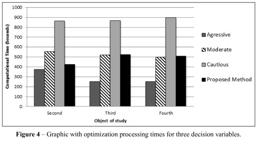
Similarly, Figure 4 shows a comparison between the necessary processing times considering three decision variables, for the optimization of the second, third and fourth objects of study. It can be noted that, for three decision variables, the proposed optimization method was faster or similar to the processing times of the moderate and cautious profiles of SimRunner^®. Thus, it can be asserted that the proposed optimization method is adequate for the simultaneous manipulation of three decision variables. Thus, as in the prior case, the proposed method was slower than the commercial optimizer's aggressive profile.

Figure 5 shows the comparison between the necessary processing times considering four decision variables, for the optimization of the third and fourth objects of study. It can be noted that for four decision variables, the proposed optimization method was faster than the processing times of the moderate and cautious profiles of SimRunner^®. Thus, it can be asserted that the proposed optimization method is adequate for the simultaneous manipulation of four decision variables. Thus, as in the prior case, the proposed method continued to be slower than the commercial optimizer's aggressive profile.

Figure 6 shows the comparison between the necessary processing times considering five decision variables, for the optimization of the fourth analyzed study object. It can be noted that, for five decision variables, the proposed optimization method was faster than the processing times of the moderate and cautious profiles of SimRunner^®. Thus, it can be asserted that the proposed method of optimization is adequate for the simultaneous manipulation of five decision variables. In relation to the aggressive profile, the proposed method remained slower, despite the difference between the two having fallen.

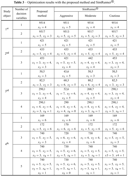
Now that the proposed method's behavior has been compared to the commercial optimization software profiles in terms of convergence time, the results attained are presented in Table 3. The results are grouped, and each study object's optimization results are presented, considering optimization with the proposed method and the three SimRunner^® (Aggressive, Moderate and Cautious). In Table 3, the value found using simulation optimization (objective function value) and the values found for each decision variable are shown for each study object and the number of decision variables in each analysis.

Table 3

The optimization profile reflects the number of possible solutions that SimRunner^® will examine. The cautious profile considers the greatest number of solutions and is the most complete in its search for optimal solutions. The aggressive profile works with small populations, thus permitting a faster convergence while in turn, sacrificing response quality. Finally, the moderate profile presents a balance between the Cautious and Aggressive profiles (SimRunner User Guide, 2002).

Thus, the proposed method is able to reach the same level of efficiency as the optimization software SimRunner^® and its profiles Cautious and Moderate, while reaching responses of equal quality or better than the Aggressive Profile. The proposed method is also more efficient thanthe commercial software in terms of convergence time, with the exception of models with only one response variable.

In reference to the profiles of SimRunner^®, response quality improved from the aggressive to cautious profiles. It can be verified that the improvement seen in the SimRunner^® profiles is directly related to the time necessary to arrive at the result. However, the best response was found using the proposed optimization method.

7 CONCLUSION AND CONTRIBUTIONS FROM THE STUDY

This article's contribution was to evaluate the proposed optimization method for discrete-event simulation models, applied to manufacturing systems, and its capability in reaching the results in the fastest form and with the same quality, when compared with commercial optimization software.

Despite the proposed method being based in metaheuristics (genetic algorithms), and therefore not being able to assert that the result found is the global optimum, the method did show itself to be as efficient as the commercial software (SimRunner^®) used as a basis for this study, while also achieving this results much faster in the majority of cases.

Four objects of study were utilized in the application of the proposed optimization method. The results found were compared with the commercially available optimization instrument, known as SimRunner^®, through the optimization methodology for discrete-event simulation models proposed by Harrel, Ghosh & Bowden (2000). In relation to the quality of the results, the proposed optimization method showed itself to be as effective as SimRunner^®.

For a single decision variable, the proposed optimization method shows itself to be less efficient. For two decision variables analyzed simultaneously, the method presented greater or equal efficiency. However, for three or more decision variables analyzed simultaneously, the proposed method of optimization is always more efficient.

When compared to the cautious profile of SimRunner^®, the proposed optimization method for the first object of the study, considering two decision variables, was around 46% faster. In relation to the second study object, considering three decision variables, the method was around 51% faster. For the third study object, considering four decision variables, the method was around 59% faster. Finally, for the fourth study object, considering five decision variables, the method was around 80% faster.

Likewise, when compared to the moderate profile of SimRunner^®, the proposed optimization method for the first study object, considering two decision variables, was around 38% faster. In relation to the second study object, considering three decision variables, the method was around 24% faster. For the third study object, considering four decision variables, the method was around 23% faster. Finally, for the fourth study object, considering five decision variables, the method was around 50% faster.

The proposed method shows itself to be valid for the outlined conditions established for this study, which consist in the manipulation of discrete, deterministic and integer decision variables.

It should be mentioned here that, in spite of the method not bringing an altogether new contribution to operational research, it does present an alternative to the existing optimization technique available on the market, which is capable of quickly optimizing simulation models while still offering high-quality solutions.

ACKNOWLEDGMENTS

The authors would like to thank the Federal University of Itajuba (UNIFEI), Sao Paulo State University (UNESP) and Padtec Optical Components and Systems. Thanks are also due to the Brazilian Federal Research Funding Agencies CAPES, CNPq and FAPEMIG.

• [1] AL-AOMAR R & AL-OKAILY A. 2006. A GA-based parameter design for single machine turning process with high-volume production. Computers & Industrial Engineering, 50: 317-337.
• [2] APRIL J, GLOVER F, KELLY JP & LAGUNA M. 2003. Practical introduction to simulation optimization. In: Proceedings of the Winter Simulation Conference, New Orleans, LA, USA.
• [3] BANKS J, CARSON JS, NELSON BL & NICOL DM. 2005. Discrete-event Simulation. 4^th ed. Upper Saddle River: Prentice-Hall.
• [4] BANKS J. 2000. Introduction to Simulation. In: Proceedings of the Winter Simulation Conference, Orlando, FL, USA.
• [5] BANKS J. 2001. Panel Session: The Future of Simulation. In: Proceedings of the Winter Simulation Conference, Arlington, VA, USA.
• [6] DAMASO VC & GARCIA PAA. 2009. Testing and preventive maintenance scheduling optimization for aging systems modeled by generalized renewal process. Pesquisa Operacional, 29: 563-576.
• [7] FU MC. 2002. Optimization for Simulation: Theory vs. Practice. Informs Journal On Computing, 14: 199-247.
• [8] FU MC, ANDRADÓTTIR S, CARSON JS, GLOVER F, HARRELL CR, HO YC, KELLY JP & ROBINSON SM. 2000. Integrating optimization and simulation: research and practice. In: Proceedings of the Winter Simulation Conference, Orlando, FL, USA.
• [9] GEN M & CHENG R. 1997. Genetic algorithms and engineering design. New York: John Wiley and Sons.
• [10] GOLDBERG DE. 1989. Genetic Algorithms in Search, Optimization, and Machine Learning.Redwood City: Addison-Wesley Publishing Company, Inc.
• [11] GOLFETO RR, MORETTI AC & SALLES NETO, L. 2009. A genetic symbiotic algorithm applied to the one-dimensional cutting stock problem. Pesquisa Operacional, 29: 365-382.
• [12] GONG DW, HAO GS, ZHOU Y & SUN XY. 2007. Interactive genetic algorithms with multi-population adaptive hierarchy and their application in fashion design. Applied Mathematics and Computation, 185: 1098-1108.
• [13] HAO Q & SHEN W. 2008. Implementing a hybrid simulation model for a Kanban-based material handling system. Robotics and Computer-Integrated Manufacturing, 24: 635-646.
• [14] HARREL CR, GHOSH BK & BOWDEN R. 2000. Simulation Using Promodel. New York: McGraw-Hill.
• [15] HOLLAND JH. 1992. Adaptation in Natural and Artificial Systems. Cambridge: MIT Press.
• [16] JIA HZ, FUH JYH, NEE AYC & ZHANG YF. 2007. Integration of genetic algorithm and Gantt chart for job shop scheduling in distributed manufacturing systems. Computers & Industrial Engineering, 53: 313-320.
• [17] KAVEH A & SHAHROUZI M. 2007. A hybrid ant strategy and genetic algorithm to tune the population size for efficient structural optimization. Engineering Computations, 24: 237-254.
• [18] KESKIN BB, MELOUK SH & MEYER IL. 2010. A simulation-optimization approach for integrated sourcing and inventory decisions. Computers & Operations Research, 37: 1648-1661.
• [19] KEYSA AC & REESB LP. 2004. A sequential-design metamodeling strategy for simulation optimization. Computers & Operations Research, 31: 1911-1932.
• [20] LAW AM & KELTON WD. 2000. Simulation modeling and analysis. 3^rd ed. New York: McGraw-Hill.
• [21] LAW AM & MCCOMAS MG. 2002. Simulation-Based Optimization. In: Proceedings of the Winter Simulation Conference, San Diego, CA, USA.
• [22] MA Y & ZHANG C. 2008. Quick convergence of genetic algorithm for QoS-driven web service selection. Computer Networks, 52: 1093-1104.
• [23] MITCHELL M. 1996. An Introduction a Genetic Algorithm. Cambridge: MIT Press.
• [24] MONTEVECHI JAB, LEAL F, PINHO AF, COSTA RFS, MARINS FAS, MARINS FF & JESUS JT. 2008. Combined use of modeling techniques for the development of the conceptual model in simulation projects. In: Proceedings of the Winter Simulation Conference, Miami, FL, USA.
• [25] MONTEVECHI JAB, PINHO AF, LEAL F, MARINS FAS & COSTA RFS. 2008. Improving a process in a Brazilian automotive plant applying process mapping, design of experiments and discrete events simulation. In: Proceedings of the 20 Symposium Europeo de Modelado y Simulacion, Briatico, Italy.
• [26] MONTEVECHI JAB, PINHO AF, LEAL F & MARINS FAS. 2007. Application of design of experiments on the simulation of a process in an automotive industry. In: Proceedings of the Winter Simulation Conference, Washington, DC, USA.
• [27] OPTQUEST FOR ARENA USER'S GUIDE. 2002. Rockwell Software Inc.
• [28] SIMRUNNER USER GUIDE. 2002. ProModel Corporation: Orem, UT. USA.
• [29] TRIOLA MF. 2006. Elementary Statistics. 10^th ed. Upper Saddle River: Pearson Education.
• [30] TUBINO DF. 1999. Sistemas de produçăo: a produtividade no chăo de fábrica. Porto Alegre:Bookman.
• [31] TYNI T & YLINEN J. 2006. Evolutionary bi-objective optimization in the elevator car routing problem. European Journal of Operational Research, 169: 960-977.
• [32] WU F, DANTAN JY, ETIENNE A, SIADAT A & MARTIN P. 2009. Improved algorithm for tolerance allocation based on Monte Carlo simulation and discrete optimization. Computers & Industrial Engineering, 56: 1402-1413.
• [33] YANG T. 2009. An evolutionary simulation-optimization approach in solving parallel-machine scheduling problems - A case study. Computers & Industrial Engineering, 56: 1126-1136.
• [34] ZENG Q & YANG Z. 2009. Integrating simulation and optimization to schedule loading operations in container terminals. Computers & Operations Research, 36: 1935-1944.

Publication Dates

• Publication in this collection
  30 Nov 2012
• Date of issue
  Dec 2012