Black swans in the brazilian stock market

Black swans in the brazilian stock market

Hugo Jacob Lovisolo^I; Ricardo Pereira Câmara Leal^II,*

^IChief Executive Officer at Notoria HB - Soluções Inteligentes, R. Alexandre Ferreira, 291, 22470-220 Rio de Janeiro, RJ, Brazil. Phone: [phone]. E-mail: [e-mail]

^IIFull Professor of Finance at the Coppead Graduate School of Business, Federal University of Rio de Janeiro - UFRJ, R. Pascoal Lemme, 355, 21941-918 Rio de Janeiro, RJ, Brazil. Phone: [phone].E-mail: [e-mail]

ABSTRACT

This study analyzes extreme values in the daily returns of 45 Brazilian stocks between 2 January 1995 and 18 March 2009. The incidence of observations outside the range of three standard deviationsfrom the mean is at least five times greater than under the normal distribution. The occurrence of extreme values in the upper tail is 1.13 times higher than in the lower. The average of the extreme positive returns is higher than that of extreme negative returns. Half percent of the days determined the outcome of the investment. Extreme values are at least ± 7%. Investors should assess whether they will keep their holdings when returns of such magnitude occur. The characteristics of empirical distributions of stock returns favor the passive investor and the use of weight constraints in portfolio allocation models.

Keywords: extreme values, normal distribution, stock risk and return.

1 INTRODUCTION

It is a well-known fact that the returns of financial assets are not normally distributed. Mandelbrot (1963) showed that financial returns have a stable Pareto distribution with α less than 2, which implies an unknown variance and makes the assumption of normality difficult. It is not valid to assume that 68.26% of observations are found between ±1σ (standard deviation), 95.44% between ±2σ , and 99.73% between ±3σ. Investors may underestimate their risk exposure if they assume that returns follow a normal distribution. This creates considerable problems for the classic mean-variance optimization proposed by Markowitz (1952) because it presumes that returns follow a normal distribution.

The consequences of the normality assumption may also vary according to the time horizon of an investment. Values are concentrated in the tails of the distribution and clustered around the mean when the distribution of returns is leptokurtic. As a consequence, Estrada (2008, 2009) affirms that returns from a few days are decisive determinants of the value accumulated in a stock portfolio. The impact of these extreme values may possibly be reduced if the investment horizon is longer. Perhaps a long-term investor is not very concerned about short-term fluctuations if changes in asset prices tend to balance out after long periods. Long-term investors thus consider that the distribution of returns is Gaussian, in which only the mean and variance of the distribution matter. Short-term investors, however, believe that their gains are obtained during large market fluctuations.

The leptokurtosis of returns produces what Taleb (2007) called "black swans": rare events with a great impact. According to the author, understanding the reasons behind extreme variations in asset values and their effects on investment returns enables investors to protect themselves against catastrophic losses and achieve higher returns than those obtained by investors who expose themselves to high volatility. Haugen & Baker (1996) affirm that high volatility assets do not provide the highest historical returns. Tversky & Kahneman (1991) conclude that the probability of loss has a greater influence on the preferences of investors than potential gains. DeMiguel et al. (2009) present evidence that has devastating implications for mean-variance optimization and many of the subsequent refinements designed to deal with the problem of optimization input parameters error. They compared 14 methods for obtaining the weights of efficient portfolios - those with greater expected returns for each level of risk - and concluded that none of them is superior to the naïve strategy of investing an equal amount in each asset.

This study takes these findings as its starting point to describe the behavior and financial impact of extreme stock returns in the Brazilian market. Estrada (2008) affirms that being out of the market in the few days of the best performance of emerging market stocks bring serious financial consequences to investors. This article draws from the recent portfolio allocation literature and its descriptive findings to suggest how investors may acquire a better understanding of the risks to which they are exposed and which usable and practical portfolio models better fit the characteristics of the data, thus increasing their probability of gains, and also points out the limitations of the traditional mean-variance optimization.

The characteristics of the distribution of returns, as inputs for portfolio decision making, are important for the design of the most adequate methods to handle the data as well as for the interpretation of the outcomes. We hope that this paper contributes to this literature by exposing important distributional characteristics of the Brazilian data and their implications for portfolio selection methods that investors in Brazil and wherever data show similar patterns can use.

This article proceeds with an exam of the previous literature in Section 2, the description of the sample and method in Section 3, and the discussion of the results in the following section. Section 5 concludes.

2 BACKGROUND

Taleb (2007) affirms that a great deal of the knowledge and facts that make a difference, in the case of both financial returns and daily life, are still unknown. The appearance of a "black swan" changes perception of people about a phenomenon. Inferences based on the normality assumption presume a distribution of information that may not be consistent with what is observed. In an article about the implications of the 2008 financial crisis for the theory of finance, The Economist (2009) quoted Myron Scholes as saying that many of the models used in financial markets were good but their input parameters were faulty because they reflected a view of the world that underplayed risk. Scholes affirmed that systemic risk was not duly taken into account and that decisions regarding exposure to risk made individually in each institution did not adequately consider the relations between different types of assets and the similar steps taken by these same institutions to cut their losses. Perhaps the magnitude of systemic risk was one of the "black swans" of the 2008 crisis. However, its lessons are being learnt. The all-embracing and severe Dodd-Frank Law, approved by the US Congress at the end of 2009, introduced a "regulator" of systemic risk, the Financial Stability Oversight Council, which, according the The Economist, was also being considered by various other countries.

The use of mathematical models in portfolio selection decisions has been the object of seminal articles published in management science/operations research periodicals, as illustrated by Osborne (1959), Sharpe (1963), Fama (1965), Brada et al. (1966), and Ziemba et al. (1974). More recent articles by Huddart et al. (2009), Yang et al. (2010), and Turner & Weigel (1992), among others, and several chapters of the series titled "Handbooks in Operations Research and Management Science" published by Elsevier, of which the portfolio theory survey by Constantinides & Malliaris (1995) is good example, indicate that the topic is current in the field. The Brazilian operations research literature also includes articles concerned with the distribution of financial assets returns, their extreme values, and portfolio selection, as exemplified by Costa & Baidya (2001), Moretti & Mendes (2003), and Ferreira et al. (2009).

Emerging markets and Brazilian return data analysis have been performed in the literature, with a particular interest in non-normality and extreme values. Ribeiro & Leal (2002) analyzed the fractal structure of emerging markets and, as would be expected, discarded the normality hypothesis in favor of more general cases of stable Pareto distributions. Torres et al. (2002) performed a careful investigation into the informational efficiency of the Brazilian stock market and rejected both the linearity and the normality of observed returns. Costa & Baidya (2001) arrived at similar conclusions in their study of the behavior of six of the more liquid shares in the Brazilian stock market and posit that returns are linearly and non-linearly dependent, but do not succeed in fitting models to their autocorrelated sample. Moretti & Mendes (2003) analyzed the problems of fitting bivariate extreme value models to financial data, Brazilian and foreign, to account for simultaneous extreme values.

Estrada (2009) affirmed that emerging markets are volatile and may surprise investors in a variety of ways. He asserts that adopting a short-term strategy is not the best way of dealing with risk because it depends on the investor skill to synchronize buying and selling operations with the fluctuations in the market. Estrada (2008) considered that a long-term passive strategy constitutes the most profitable course of action because it offers the best chance of not being out of the market during the few days that will really make a difference to the final result. Being out of the market on the few days that stocks perform better may be disastrous to investors.

The non-normality and high incidence of extreme values in stock market return series also has consequences for portfolio allocation and its models. DeMiguel et al. (2009) present evidence that a simple equally weighed portfolio, in which each asset corresponds to a proportion of 1/n of the initial investment, for n assets, beats all of the 14 more sophisticated portfolio allocation models using US and other developed countries data that they employed. The naive 1/n portfolios outperformed even some robust portfolio allocation models included in their tests. The authors concluded that a window of 3,000 months would be necessary for a mean-variance optimization method to beat the naive portfolio.

DeMiguel et al. (2009) also considered the global minimum variance portfolio (GMVP), that does not demand expected return inputs. Thomé Neto et al. (2011) analyzed the performance of the GMVP and 1/n portfolios according to several constraints on the maximum weights an asset could attain. They concluded that the GMVP with no short selling and weights limited to no more than 10 percent and the 1/n offered better risk adjusted performance than other GMVP allocations with larger weight constraints or unconstrained, the Ibovespa index, and several actively managed stock funds. They found no statistical difference between the performance of 1/n portfolios and the GMVP portfolios with weights constrained to 10 percent. The authors studied the returns of the most liquid Brazilian stocks between January 1998 and December 2008, with rebalancing every four months, in synchrony with the Ibovespa index rebalancing. Behr et al. (2013) considered the role of constraints in a comparative analysis of optimized portfolios relative to naive 1/n portfolios. Their constraints were based on shrinkage theory. They find that their approach was the only one to outperform the Sharpe ratio of naive allocations.

Extreme values may bring about very serious financial consequences for investors. Stock return data contains many more extreme values than the predicted under a normal distribution. Being absent from the market in the best return days yields a mediocre financial performance. Extreme returns also affect the weights of optimized portfolios while weight constraints, ad hoc or not, alleviate these problems. Equally weighed portfolios are a competitive solution for practical portfolio allocation problems.

3 SAMPLE AND METHOD

The analysis performed here was restricted to the Brazilian market and the methodology used drew on Estrada (2008). The study focused on the most liquid stocks because the distributions of their returns should have a lower propensity to diverge from normality than those of smaller companies and lightly traded stocks. The period studied began on the first trading day of the year following the Real Plan (Jan. 2, 1995) and ended on March 18, 2009 and included 2527 trading days. The study initially took on 50 stocks that were traded on more than 80% of the days in the period and whose individual volume amounted to more than 0.1% of the total. When a company had more than one class of stock traded, the most liquid preferred stock was selected because it was usually more actively traded than the common stock. The inclusion of one stock per company aimed at reducing the correlation between the stocks chosen, given possible similarities in the behavior of stocks belonging to the same issuer.

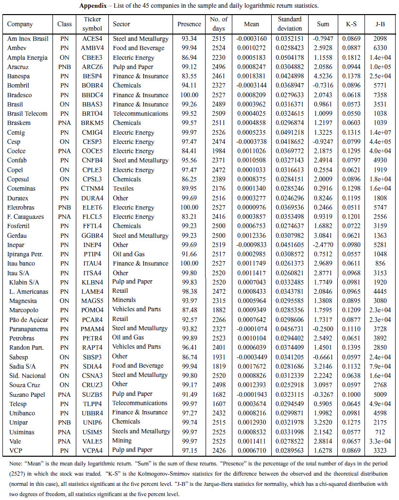
Closing stock prices, adjusted for dividends and other payments, were taken from the Bloomberg^®system. The stocks of some companies have a smaller number of daily observations because they were not traded on all days of the period studied. Five companies were excluded from the sample because their stock prices were not quoted for long periods (Light ON) or because their price series had consistency problems that could not be resolved by the data provider (Celesc PNA, M.G. Poliest ON, Varig PN, and Forjas Taurus PN). The final sample included 45 companies from 13 industries. The industry with the largest number of companies was the electricity energy, with seven companies, followed by steel and metallurgy with six, the financial and insurance and chemical industries with five, pulp and paper with four and the other nine sectors with no more than two stocks each. The appendix contains a list of companies with their ticker symbols, industry, the number and percentage of days with returns during the period and the means, standard deviations and sum of logarithmic returns for each stock in the sample.

The return of a stock i on day t (ri, t ) was calculated as the difference between the price logarithms on this day and the previous one (ln Pi, t -ln Pi, t-1). The logarithmic returns can be summed to obtain the accumulated return during a period. Logarithmic returns attenuate the effects of extreme values on the form of their empirical distribution, making it more similar to a normal distribution.

The frequency of observed returns was compared with those expected under normality for various areas around and more distant from the mean. The result of the investment undertaken when an investor was not long on the stock on its worst and best days was compared with that of a passive investor who followed a buy and hold strategy. The study examined the 1, 5, 10, 20 and 50 worst or best days. The aim was to investigate whether a few daily returns determined the final result of the investment even when its time horizon was long.

Let T be the number of trading days during a certain period, T_Gthe set of N days with the largest gains during T , T_Pthe set of N days with the largest losses during T , with N equal to 1, 5, 10, 20 and 50 days. The percentage gain of stock i during period T (G_i , T ) due to not being invested during the N worst days of the period is given by equation 1. The percentage loss recorded by stock i during period T (P_i, T ) due to not being invested during the N best days of the period is given by equation 2. The denominator of the two equations is the return achieved by a passive investor who remained invested in the stock throughout the whole period. The numerator of equation 1 represents the return of an investor who was not long on the stock precisely on the days when it had its lowest returns. The numerator of equation 2 represents the return achieved by an unlucky investor who was not long on the stock exactly on the days when it had its best returns.

The distance (Di ) of the mean return of the set of extreme observations (_e, i ) in relation to the mean return of a stock (_i ) during the period, in units of its standard deviation (σ_i ), was calculated according to equation 3. The set of extreme observations considered are represented by T_G, the set of N days with the largest gains, and T_P, the set of N days with the largest losses, with N equal to 1, 5, 10, 20 and 50 days.

4 RESULTS

Table 1 presents a summary of the descriptive statistics of the logarithmic returns of each stock. The detailed results for each stock can be obtained from the authors. The appendix contains a list of companies with some of their statistics. There were large differences between the companies in nearly all cases of the descriptive statistics shown. The average of the sum of logarithmic returns during the period was 1.448, or 325.5%, representing the result achieved by a passive investor who invested in an equally weighted portfolio containing the shares in the sample. Seven share shad negative mean daily returns. The mean of daily logarithmic returns of the best performing stock was nearly 19 times greater than that of the stock with the lowest mean positive return. The mean of the five best performing stocks was 677% greater than the mean of the five stocks with the lowest positive appreciation.

The largest standard deviation in the sample was almost twice as high as the lowest. The correlation between the standard deviations and the mean of the logarithmic returns was -0.39 and suggested an inverse relation between the returns achieved and historical volatility, as indeed found by other authors. As a matter of fact, if the relationship between the returns achieved and historical volatility were monotonic and positive, investors would only choose riskier assets. The coefficient of correlation between these two metrics was negative but not very low and suggested that cases of high risk accompanied by large returns also existed among the companies in the sample. A careful examination of the appendix confirms this. It may be the case that investors who are willing to engage in frequent short-term buying and selling of shares should seek shareswith the highest standard deviations, whereas long-term investors should perhaps choose shareswith lower standard deviations.

The high coefficients of kurtosis and asymmetry revealed the large distance between the logarithmic distributions of returns and normal distributions, whose coefficients of kurtosis and asymmetry are three and zero respectively. Average kurtosis was six times greater than three and minimum and maximum values were 2.605 and 370.75 respectively. Kolmogorov-Smirnov and Jarque-Bera normality tests, whose results are reported in the appendix, also rejected the normality hypothesis for all companies in the sample. Sixteen companies had negative asymmetry coefficients and twenty-nine had positive ones. The average was close to zero, but few stocks had coefficients close to zero. Positive asymmetry is obviously desirable.

Table 2 presents the number of extreme observations of logarithmic returns compared to the number of extreme values expected if the distribution was normal. Extreme values are those that fall outside three standard deviations above or below the mean, where no more than 0.27% of observations should be under normality. The number of extreme values expected for each stock is the result of the sum of the number of daily observations for the stock in the sample multiplied by 0.00135, which is the proportion of the unit area under the curve in each area above or below three standard deviations from the mean. The average frequency of extreme values was at least five times greater than would be expected under normality. The incidence of extreme values in the upper tail was 1.13 times greater than in the lower one, which had already been indicated by the greater occurrence of positive asymmetry coefficients. The stock with the lowest number of extreme values had 1.47 more than would be expected if the distribution of daily returns were normal. Figure 1 presents the frequency histogram for the ratio of observed to expected return sabove or below three standard deviations from the mean for the 45 stocks in the sample. For most of them, the frequency of extreme values was between four and seven times greater than what would be expected under normality.

Table 3 shows that the influence of a handful of daily returns is decisive for investors. On average, the result of an investment over a period of 2300 days - practically ten years - was determined by around half a percent of these days. If an unlucky investor managed to be absent on the days when a stock enjoyed its best returns, his/her accumulated wealth would be 78% lower than a passive investor who remained invested throughout the period. A lucky investor who managed not to be invested on the days when the stock had its lowest returns would, on average, have earned five times more than a passive investor. Naturally, very few investors are so lucky or unfortunate in the real world.

What this all shows is that the result of an investment in stocks is determined by a handful of devastating or dazzling days. Mean absolute returns of the ten most devastating days were nearly 230 times greater than the mean returns of all days and were around -14% per day. The mean accumulated logarithmic return on all days in Table 1 was 1.448. The sum of the mean returns of the ten worst days was approximately -1.5. The difference between these two values was slightly negative and represented the sum of the mean returns in all other days. The sum of the ten best daily returns was approximately 1.6. By subtracting this value from the sum of the mean returns of all other days, one obtains the sum of mean returns of the other days, which was also negative. The mean daily returns of the 50 most devastating days was -9.5%. The mean extreme minimum logarithmic return was around -7%, in the case of losses, and 8% in the case of gains. Daily variations of this size should put an investor on alert. The distance of ±3σ is easily surpassed on days when the market experiences movements of great magnitude. The average distance of the extreme values of each stock from the mean is nearly always greater than 3σ.

It is clear that investors will not be able to synchronize their buying and selling in an attempt to minimize the effects of days when stocks experience their sharpest declines and most will only know about this after the fact. Nevertheless, the results described are of practical importance even after they have happened. Perhaps investors will conclude that it is time to sell the stock when they realize that they were invested during the few dazzling days of a stock, when, for example they achieved returns of 10% or more on ten days during this period. It is possible that things will not get any better and the risk of remaining invested may no longer be worthwhile. On the other hand, investors who remained invested during a period with many disastrous days, with losses of 7% or more on each one, may also decide to sell because they have come to theconclusion that the chances of recovery are small.

If the more volatile days - both dazzling and disastrous - are lumped together, as, for example, Torres et al. (2002) and Costa & Baidya (2001) concluded by finding that conditional volatility models adjust well to Brazilian stock returns, then it would be better to remain invested, given that the positive asymmetry of returns may lead to a net positive result due to the fact that the

losses incurred on disastrous days will be offset by the gains obtained on dazzling ones. The best of worlds, however, would be a situation in which disastrous days were not lumped togeth erwith the dazzling days, and have not yet occurred, and investors decide to sell after realizing that they were invested on the best days. It is important that investors observe highly volatile dayscarefully in order to draw their conclusions and take their decisions accordingly. They should take note of daily returns of ±7% because they are the black swans.

Table 4 presents a summary of the comparisons made between the number of occurrences ofobservations in selected areas of the empirical distribution and the number expected under normality. An examination of Table 4 confirms the leptokurtic characteristics of the empirical distributions, given that both the percentage of values observed in the area close to the mean and the percentage of observations in the tails were greater than in a normal distribution. In the intermediate areas, on the other hand, the percentage of observations was lower than in the normal curve.

5 CONCLUSIONS

It is well known that the empirical distributions of returns do not follow a normal distribution.This article attempted to obtain an exact notion of this difference and measures its impact in relation to the financial results obtained by passive investors. The discrepancies found were enormous and their impacts devastating. The study analyzed the daily logarithmic returns of 45 Brazilian shares between 2 January 1995 and 18 March 2009. The stocks were selected according to their liquidity and market presence.

The descriptive statistics varied considerably from stock to stock. The average of the mean return of each stock amounted to 16.5% a year and the standard deviation of the lowest volatility stock was half that of the highest volatility stock. There was a negative correlation between the mean and the standard deviation of returns. Average kurtosis was six times greater than that of the normal curve. Although logarithmic returns were used for the analysis, the asymmetry of empirical distributions was frequently positive. The incidence of observations at a distance of more than three standard deviations from the mean (±3σ ) was, on average, five times greater than would be predicted by a normal curve. The incidence of extreme values in the upper tail was 1.13 times greater than in the lower tail. The incidence of extreme values in the time series of returns of most stocks analyzed was four to seven times greater than would be expected under the normality hypothesis.

Most returns were situated within an interval of more or less one standard deviation in relation to the mean (±1σ ). This meant that volatility was low on most days, or 77.95%, which was lower than would be expected in a normal distribution, in contrast to the other days (22.05%) when extreme returns were much more numerous than would be predicted by a normal distribution. In the case of the normal distribution, 31.8% of returns would fall outside an interval of ±1σ andonly 0.27% of them would be extreme, situated at a distance of ±3σ . The percentage of extreme values in a normal distribution would be 0.85% (0.27% ÷ 31.8%). The empirical results showed

that only 22.05% of returns were outside an interval of ±1σ and approximately 1.45% of them were extreme. In the positive tail, given that the result was higher than 1σ , there would be an approximately 7.45% chance that it would be extreme (0.79% ÷ 10.59%). In the negative tail, as the result was lower than -1σ there would be a 6.58% chance that it would be extreme (0.66% ÷ 10.03%). Even though 7.45% and 6.58% seem to be small percentages, they are, respectively, 8.75 and 7.75 times the 0.85% that would be expected in the case of a normal distribution.

Extreme values have a decisive influence on the result of an investment. In this case, around half percent of days practically determined the result of an investment during a period of more than 2300 trading days, on average, for each stock. The accumulated mean return of "normal" days in the area between the tails was slightly positive. The returns obtained by a lucky investor who was not invested on the ten worst days of the period were five times greater than those achieved by a passive (buy and hold) investor. An unfortunate investor, who managed not to be invested during the ten best days in the period, obtained four times less than a passive investor. The magnitude of the extreme minimum return was on average nearly ±7%. Daily returns with magnitudes that are equal to or greater than this should serve as a warning to investors, as they indicate the presence of an extreme value.

Of course one cannot expect an investor to be able to foresee the days when extreme values will occur, but an investor can observe that an extreme value has occurred and make an appropriate investment decision. If extreme positive and negative values are lumped together, perhaps it is best to remain invested and rely on the positive asymmetry of empirical distributions to ensure that extreme positive values more than offset negative values, bearing in mind that, when only normal days are considered, the result of an investment is, on average, slightly negative. This is the strategy followed by a long-term passive (buy and hold) investor.

If positive and negative values are not clearly lumped together, investors who conclude that they have already obtained their portion of extremely positive daily returns for a stock, which will not amount to much more than half a percent of trading days during a reasonable investment period - or around one or two per year - should perhaps sell the stock, particularly in order to avoid being exposed to the possible occurrence of extreme negative returns, if they have not already occurred. Investors that experienced extremely negative returns, thus reducing the result of theirinvestment significantly, should consider selling their shares because the probability of recoverymay be small.

These simple heuristics based on the historical occurrence of extreme values may not yet be clear for most investors. They may not realize that the returns obtained from shares are provided by a handful of days with a dazzling performance. Losses are also due to a handful of disastrous days. A well-known feature of investor behavior is a reluctance to realize losses, even if they are catastrophic. The results presented here provide an order of magnitude for investor heuristics, especially regarding the difficult decision to sell. Positive or negative returns of seven percent or more on only half percent of the days of an investment period that is not too short may representa watershed in the perception of market possibilities of an investor, convincing him/her that the time has come to take profits or realize losses, and go ahead with other investments. The mean returns recorded during the other days do not, on average, contribute significantly to the result of the investment. The message is also clear for options investors - the risk of taking short positions may be much greater than imagined, particularly when one considers that the main options pricing model - the Black and Scholes model (1973) - is based on the assumption that logarithmic returns are normally distributed.

These results also have implications in the use of portfolio optimization procedures, which have been discussed in the literature. DeMiguel et al. (2009) defend the view that simple rules of diversification, such as investing in an equally weighted portfolio, produce better results than more sophisticated ways of determining these weights. Even the use of robust modeling, which adds substantial complexity to the portfolio allocation procedure, does not warrant better results than traditional optimization for all risk levels, as discussed by DeMiguel et al. (2009) and Mendes & Leal (2005).

Thomé Neto et al. (2011) highlighted the qualities of naive diversification and of the global minimum variance portfolio for Brazilian stocks, whose weights do no depend on expected returns. Behr et al. (2013) point out that portfolio optimization performs better under reasonable shrinkage derived constraints. Mendes & Leal (2005) show that extreme returns distort the covariance matrix and leads to less reliable weights obtained from classical portfolio traditional optimization techniques. Nevertheless, as a consequence to investors in Brazil, the presence of extreme returns implies that investors should use weight constraints and that those unable or unwilling to apply optimization may rely on equal weights to attain good results, as long as they rebalance their portfolios a few times per year.

It is reasonable to believe that this also applies to allocations of assets among different asset classes. One of the main ways investors can protect themselves from the devastating effect of negative extreme values is never to allocate all their wealth in stocks and invest an important portion in low volatility assets. According to DeMiguel et al. (2009), in Babylon, in the fourth century A.D., rabbi Issac bar Aha proposed that assets should be allocated in the following way: "One should always divide wealth into three parts: a third in land; a third in goods; and a third for use". Peter Lynch, the legendary manager of Fidelity Investment's Magellan Fund between 1977 and 1990, in the USA, echoing the rabbi's wisdom, said in a TV interview that the ideal allocation would be a third in shares, a third in long-term bonds, and a third in short-term bonds.

Received December 15, 2011

Accepted January 23, 2013

^Appendix

• [1] BEHR P, GUETTLER A & MIEBS F. 2013. On portfolio optimization: imposing the right constraints. Journal of Banking & Finance, 37:1232-1242.
• [2] BLACK F & SCHOLES M. 1973. The pricing of options and corporate liabilities. Journal of Political Economy, 81:637-654.
• [3] BRADA J, ERNST H & VAN TASSEL J. 1966. The distribution of stock price differences: Gaussian after all? Operations Research, 14:334-340.
• [4] CONSTANTINIDES GM & MALLIARIS AG. 1995. Portfolio Theory. In: Handbooks in Operations Research and Management Science - Finance, 9 [edited by JARROW RA, MAKSIMOVIC V & ZIEMBA WT], Elsevier, 1-30.
• [5] COSTA PHS & BAIDYA TKN. 2001. Propriedades estatísticas das séries de retornos das principais ações brasileiras. Pesquisa Operacional, 21:61-87.
• [6] DEMIGUEL V, GARLAPPI L & UPPAL R. 2009. Optimal versus naive diversification: how inefficient is the 1/N portfolio strategy? The Review of Financial Studies, 22:1915-1953.
• [7] EFFICIENCY AND BEYOND. 2009. The Economist, 8640:68-69.
• [8] ESTRADA J. 2008. Black swans and market timing: how not to generate alpha. Journal of Investing, 17:20-34.
• [9] ESTRADA J. 2009. Black swans in emerging markets. Journal of Investing, 18:50-56.
• [10] FAMA EF. 1965. Portfolio analysis in a stable Paretian market. Management Science, 11:404-419.
• [11] FERREIRA RJP, ALMEIDA FILHO AT DE & SOUZA FMC DE. 2009. A decision model for portfolio selection. Pesquisa Operacional, 29:403-417.
• [12] HAUGEN RA & BAKER NL. 1996. Commonality in the determinants of expected stock returns. Journal of Financial Economics, 41:401-439.
• [13] HUDDART S, LANG M & YETMAN MH. 2009. Volume and price patterns around a stock's 52-week highs and lows: theory and evidence. Management Science, 55(1):6-31.
• [14] MANDELBROT B. 1963. The variation of certain speculative prices. Journal of Business, 36:394-419.
• [15] MARKOWITZ H. 1952. Portfolio selection. The Journal of Finance, 7:77-91.
• [16] MENDES BVM & LEAL RPC. 2005. Robust multivariate modeling in finance. International Journal of Managerial Finance, 1:95-107.
• [17] MORETTI AR & MENDES BV DE M. 2003. Sobre a precisão das estimativas de máxima verossimilhança nas distribuições bivariadas de valores extremos. Pesquisa Operacional, 23:301-324.
• [18] OSBORNE MFM. 1959. Brownian motion in the stock market. Operations Research, 7:145-173.
• [19] RIBEIRO TS & LEAL RPC. 2002. Estrutura fractal em mercados emergentes. Revista de Administração Contemporânea, 6:97-108.
• [20] SHARPE W. 1963. A simplified model for portfolio analysis. Management Science, 9:277-293.
• [21] TALEB N. 2007. A Lógica do Cisne Negro: O Impacto do Altamente Improvável. 2. ed., Best Seller, Rio de Janeiro, RJ.
• [22] THOMÉ NETO C, LEAL RPC & ALMEIDA VS. 2011. Um índice de mínima variância de ações brasileiras. Economia Aplicada, 15:535-557.
• [23] TORRES R, BONOMO M & FERNANDES C. 2002. A aleatoriedade do passeio na Bovespa: testando a eficiência do mercado acionário brasileiro. Revista Brasileira de Economia, 56:199-247.
• [24] TURNER AL & WEIGEL EJ. 1992. Daily stock market volatility: 1928-1989. Management Science, 38:1586-1609.
• [25] TVERSKY A & KAHNEMAN D. 1991. Loss-aversion in riskless choice: a reference-dependent model. The Quarterly Journal of Economics, 106:1039-1061.
• [26] YANG J, ZHOU Y & WANG Z. 2010. Conditional coskewness in stock and bond markets: time-series evidence. Management Science, 56:2031-2049.
• [27] ZIEMBA WT, PARKAN C & BROOKS-HILL R. 1974. Calculation of investment portfolios with risk free borrowing and lending. Management Science, 21:209-222.

Appendix

*

Corresponding author

Publication Dates

• Publication in this collection
  16 July 2013
• Date of issue
  Aug 2013

History

• Received
  15 Dec 2011
• Accepted
  23 Jan 2013