Abstracts
Variational Data Assimilation and Adjoint Equation Method are presented here as a general methodology designed to improve the quality of computational simulation when are given the dynamics and a set of observation of the system under study. The mathematical foundations the procedures to obtain the adjoint of a given computational program, a fundamental task in order to apply the methodology, are carefully examined.
Variational Data Assimilation; Adjoint Equations; Adjust of Trajectories
A Assimilação Variacional de Dados e o método das Equações Adjuntas são aqui apresentados como uma metodologia geral, desenvolvida para melhorar a qualidade das simulações computacionais, quando a dinâmica e um conjunto de observações do sistema em estudo são conhecidos. Os fundamentos matemáticos e os procedimentos para se obter o adjunto de um dado programa computacional, uma tarefa fundamental para a aplicação da metodologia, são cuidadosamente examinados.
Assimilação Variacional de Dados; Equações Adjuntas; Ajuste de Trajetórias
ARTIGOS
Variational data assimilation: mathematical foundations and one application
Assimilação variacional de dados: fundamentos matemáticos e uma aplicação
Paulo S. D. da SilvaI; Gudélia MoralesII; Príscila H. G. OliveiraII
ILaboratório de Ciências Matemáticas, Universidade Estadual do Norte Fluminense, RJ, Brazil
IILaboratório de Engenharia de Produção, Universidade Estadual do Norte Fluminense, RJ, Brazil
paulosd@uenf.br, gudelia@uenf.br, phgoliveira@ibest.com.br
ABSTRACT
Variational Data Assimilation and Adjoint Equation Method are presented here as a general methodology designed to improve the quality of computational simulation when are given the dynamics and a set of observation of the system under study. The mathematical foundations the procedures to obtain the adjoint of a given computational program, a fundamental task in order to apply the methodology, are carefully examined.
Keywords: Variational Data Assimilation, Adjoint Equations, Adjust of Trajectories.
RESUMO
A Assimilação Variacional de Dados e o método das Equações Adjuntas são aqui apresentados como uma metodologia geral, desenvolvida para melhorar a qualidade das simulações computacionais, quando a dinâmica e um conjunto de observações do sistema em estudo são conhecidos. Os fundamentos matemáticos e os procedimentos para se obter o adjunto de um dado programa computacional, uma tarefa fundamental para a aplicação da metodologia, são cuidadosamente examinados.
Palavras-chave: Assimilação Variacional de Dados, Equações Adjuntas, Ajuste de Trajetórias
1. INTRODUÇÃO
In the second half of the eighties, in the confluence of the spreading in West Europe of of the work made by G. I. Marchuk on Adjoint Equation Method applied to Geophysical Flux Dynamics issues, and under the strong influence of the results obtained by J. L. Lions as to systematic use of the Optimal Control Theory to systems governed by partial differential equations, in particular, in Atmospheric Flows (Talagrand, 1997), they appeared numerical methods which would become the Variational Data Assimilation operational in less than 10years.
Sensitivity Analysis, through the adjoint formalism, quickly became useful in a wide variety of research areas (Thomas et al, 2002 , 2005, Kamien and Schwartz, 1981, Reuther et al, 1996). Nevertheless, only in recent years, the Data Assimilation technique has been exploited in computational simulations not related to Numerical Weather Prediction (Elbern et al., 2007), although the method can be invaluable in computational simulations, since observations of the systems act on the numerical model as restriction which the solution must verify. One of the possible explanations for this situation might be that the high complexity of the numerical experiments of atmospheric and oceanic flows and the many peculiarities of those flows make the experiments rather accessible to the computational simulation community. Besides, with the exception of a few articles (Le Dimet and Talagrand, 1986) and books (Kalnay, 2002, Daley, 1993), the mathematical formalism is not always clearly presented. This situation is not appropriated to the development of the Variational Data Assimilation method, since important aspects for its future plans, for example, Adaptive Observations, must be placed in solid theoretical foundations.
Therefore, this work is intended to present a rigorous mathematical formulation not only for Variational Data Assimilation but also Adjoint Equation Method as well, and, as an algorithm to perform the variational assimilation of data was developed, which is also described here, both formulations can be perfectly understood.
In order to realize the numerical control of the space-time evolution of a system involving a geophysical flow it is necessary to know its initial condition, which is, the numerical counterpart of the real initial state or the initial configuration of the system under study. In the case of geophysical flows, the dimension and the geographic location of the spatial domain problems make the distribution of an observational network difficult, what causes a scarcity of data about the phenomenon studied or even turns the intial configuration unavailable for computational simulations (Talagrand, 1997). As in those flows are presented phenomena of difficult representation in a numerical model, and even in analytical models, being, in certain situations, processes highly sensitives to initial conditions variations (Lorenz, 1963), to establish an initial condition adequated for simulations, in this case, is of the paramount importance for the results.
For an adequate initial condition of the numerical experiment, one means that one which generates the numerical model states that fit, in accordance with the desired precision, the available observations. In order to decide whether or not an initial condition is appropriated to certain simulation, one should consider, in additon to the flow dynamics, the full set of observations of the system being studied. That is exactly what is performed by the methodology known as Data Assimilation (Le Dimet and Talagrand, 1986), approach in which all the knowledge on a system being analyzed, its dynamics and observations, is combined in order to produce an initial condition that minimize the error between the model generated configurations and the correspondent known configurations, in a sense to be precised later.
A problem involving geophysical flows in its discrete form produce sa very high number of variables, so that, straight away, Variational Data Assimilation is a metodology computationally intractable. A solution for this difficulty can be obtained with the use of the Adjoint Equation Method, which adequately insert the problem of the initial condition determination to simulations of geophysical flows in the domain of Optimal Control Theory (Lions, 1971), and its mathematical foundations are analyzed here with the necessary accuracy. A second consequence of the resulting metodology of combining Variational Data Assimilation with Adjoint Equation Method is the transformation of a minimization problem with restrictions, as originally proposed by the Variational Data Assimilation formalism, in a minimization problem without, what makes it possible the use of more agile routines, as L-BFGS (Liu and Nocedal, 1989), in the determination of an optimal initial condition.
The efficency of that metodology, confirmed by numerical wheather prediction operational models (Parrish and Derber, 1992), has produced, on the one hand, a tremendous increase in the scope of its applications (Elbern et al, 2007), (Kamien and Schwartz, 1981), (Reuther et al, 1996), on the other hand a continous clarification of its theoretical basis, which is necessary for the improvement of the already existing models, and for the rise of others more precise.
In the first section of this work, the mathematical foundations of two crucial methods are presented, Variational Data Assimilation and Adjoint Equation Method. In the second section, in order to fix ideas, one works with a unidimensional model which permits the exploration of several aspects of the methods used and also to develop explicitly the adjoint of a given equation. Finally, in the third section, one describes a bidimensional numerical experiment, showing with some detail (i) an algebraic formalism, fundamental in the development of a computational program to perform the experiment, formalism that has already produced, in the Computational Linear Algebra domain, a new line of investigation, known asAutomatic Differatiation (Kaminski et al, 2003) and as Automatic Adjoint Generation (Giering et al, 2005), and (ii) the structure of a FORTRAN code, created by the authors, in order to realize the Variational Data Assimilation of a flow described by the bidimensional advection-diffusion equation.
2. MATHEMATICAL FORMULATION
Definition: Let A be an open set in  n e f:A → a differentiable function. Then, ∀x ∈ A, the differential of f in x is the linear functional tal que, ∀v ∈
As df(x) is a linear functional in (n)* *, the dual vector space of n, it follows form Linear Algebra the existence and the uniqueness of the n vector, ∇f(x), such that
where <,> is the canonical inner product in
n.2.1.The Data Assimilation Method
Let S be an evolutionary system, observed during the time interval [t1,t2], from which is available a set of observations, all of them colected in the same time interval and distributed in the spatial domain of interest on S. Besides, it is known the dynamics of S. Based on those pieces of information, one wants to determine the initial condition of the modelled S, or the numerical representation of the configuration of S at the time t1 , the starting moment for a computational simulation of S generates configurations to approach, within an acceptable precision, to the available observations of S at correspondent instants of time, in order to obtain a configuration of the model at tf > t2 which reproduces the real configuration of S at time tf, also within an acceptable pricision. From a conceptual point of view, this process is similar to the Best Linear Unbiased Estimation (Sorensen, 1980) of the configuration of S at tf, given the S configurations within [t1,t2], here solved in a deterministic approach as an optimal control problem, in which the initial conditions is the control data.
At first, one considers the continuous version of the Variational Data Assimilation problem, which admits the appropriate mathematical treatment. In this case, the mathematical objects are:
(i) the system observations: S, Z:[t1,t2] × V → V, such that, ∀t ∈ [t1,t2], Zt: V → V is a differential operator defined on the vector space V provided with the inner product <,>, where [t1,t2] is the assimilation interval or assimilation window.
(ii) the dynamics of the system S, described by
Where X:[t1,t2] × V → V is the system S trajectory during the assimilation interval, [t1,t2], E={Y;Y:[t1,t2] × V → V and Y ∈ C2} and F:E → E is a differential operator.
(iii) the "weight" function W:[t1,t2] → L(V), where L(V) is the vector space of the linear operators in V, that results from the statistics information of the instruments used to collect the data on S , and that, each t ∈ [t1,t2], associate the injective linear operator
W(t): V → V
(iv) the quadratic functional
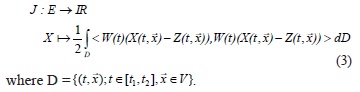
Then the Variational Data Assimilation problem is to find a trajectory of the system states S, X:[t1,t2] × V → V such that X be the solution of Equation 2 which minimize the functional Equation 3, in other words, the following minimization problem with constrait:
Problem MR: find the solution of Equation 2 minimizing Equation 3
As the solution of the Data Assimilation will be numerically obtained, it is necessary to solve its discrete version. However, this implies another difficulty: the number of resulting variables of discrete version of the equation modelling the S dynamics and its space-time domain is excessively high. Therefore, from the computational point of view, it would be very economic (and, in many problems, the only feasible way) if instead of the solution X E ∈ one searches the solution X1 ∈ E1, where E1= {X1; E1 = {X1;X1 = X {t1}×V, X ∈ E and X ∈ C2} isomorph to the set of operators in V, which could be called the space of the initial configurations of S, that minimizes the restriction of the functional J to E1. The difficulty here is the non existence of a relation between J and X1, because J is not a function of X. However, if the problem in Equation 2 is well posed, then the knowledge of X and the knowledge X1 are equivalent. The Adjoint Equation Method provides, from the relation between X and X1, the differential of the restriction of J to E1.
2.2.The Adjoint Equation Method
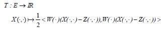
One rewrites the functional in Equation 3 as
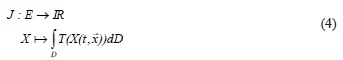
where
As the differential of J in X ∈ E is a linear functional in the Hilbert space E with the inner product
by using the Riesz' Representation Theorem (Kreyszig, 1989), one obtains, ∀ H ∈ E,
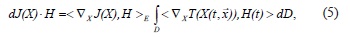
where ∇XJ e ∇XT, are the gradient of J and of T, respectively
Now, one considers the linear version of the Equation 2:
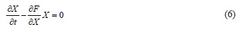
resulting from the substitution of the operator F for its first order approximation in an equilibrium point, ommited from the equation, and in which it was used the notation  for its differential, and its adjoint equation:
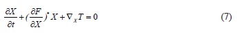
where is the adjoint of the operator
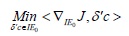
Theorem 1: Given a solution X E ∈ of MR, X1 ∈ E1, X1 = X|{t1}×V, is the solution of the following unconstraint minimization problem:
Problem MS: find δX ∈ E1 minimizing <∇ X1J, δX>.
Proof: Let Y: [t1, t2] × V → V be the solution of (7) such that Y(t2) = 0 and δX ∈ E1 a perturbation of any solution of Equation 6. Then it follows that:
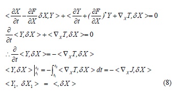
The meaning of Equation 8 must be clear: the right side of the equality is the expression of the differential of J (relative to X), dJ(X). As X1is the projection of X onto E1, the left side of Equation 8 is the expression of the differential of the restriction of J (relative to X1) to E1. By the uniqueness of the representation of the last differential as an inner product in E1, it follows that Y1 is precisely the gradient of the restriction of the funtional J to E1, that is, Y1 is the projection of ∇XJ onto E1. Then, one obtains

Therefore, using the Adjoint Equation Method, one projects the solution set C2([t1,t2] ×V ,V) onto C2({t1} ×V ,V), which represents, from the computational viewpoint,a considerable reduction in the number of variables in the discrete problem. Besides, this projection transforms a constraint minimization problem in one unconstraint problem, namely, the problem of minimizing Equation 3 with the restriction Equation 2, becomes
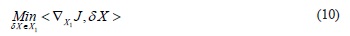
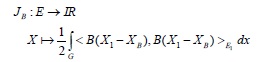
The problem MR, involving the quadratic functional J, defined in Equation 3, has the existence of its solution guaranteed but not its uniqueness. In order to obtain the uniqueness of the solution of MR, and of MS, one redefines the problem using the following quadratic functional:
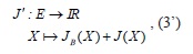
where, Xbis an available estimate of the initial configuration of X, and B ∈ L(V) is the operator determined by the available statistical information on the estimate of Xb and
Then, one obtains the following result:
Theorem 2: Given the Problem MR': find the solution of Equation 2 that minimizes Equation 3'.
There exists a unique solution of MR' and X1 = X|E1 ∈ E1 ∈ is the solution of the following unconstrait minimization problem:
Problem MS': find δX1 ∈ E1 that minimizes

Proof: It is only necessary to redefine the inner product on E as:
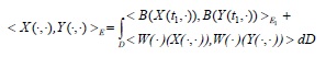
and use all the development that preceeds Theorem 1.
Let Xb be the available estimate of the initial configuration of X. The problem of optimal solution will be iteratively solved by shearching the perturbation δX1 ∈ E1 of δX ∈ E1 such that (Xb + δX) will be the solution of MS´.
3. ONE UNIDIMENSIONAL EXAMPLE:
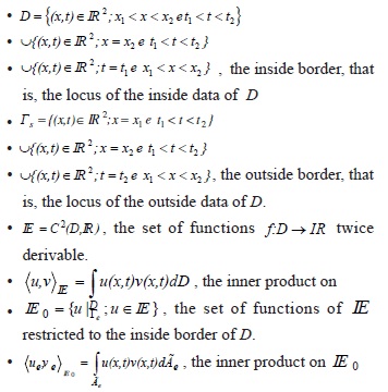
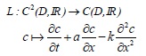
Definição: Given D = {(x,t) ∈ 2,X1 < x < x2 et1 < t < t2} and à the border of D, one defines:
One considers the following situation: a fluid (water) flowing in a river or a channel of lenght l = x2 -x1, where the window of assimilation is [t1,t2] . A certain amount of pollutant is spilled in the channel in x<x1 in the instant t1. By hypothesis, the transport of the pollutant is described by the advection-diffusion unidimensional equation.
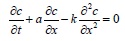
with the initial and contour conditions:
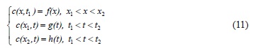
where is the water velocity, is the diffusivity coefficient and is the pollutant concentration in D.
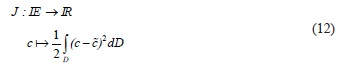
Let us supose the availability of a set of channel observations,
D →, during the time interval [t1,t2]. The Data Assimilation problem consists in finding a solution of Equation 11 that minimizes the functional
that is, one has the following problem:
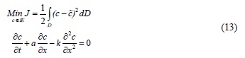
Obtaining the solution of Equation 13, one can determine the instant of time when the pollutant will reach the position x > x2, and this solves the problem of the deterministic prediction of the pollutant trajectory along the channel. If one is interested just in the position x of the front of the oil stain in relation to a reference point in one of the the channel shore, the geometry of the problem is one-dimensional.
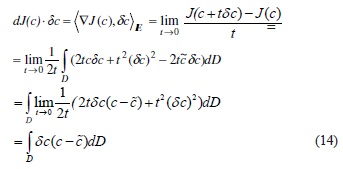
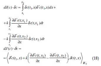
In the sets {(x,t)} ∈ 2,x = x1and t1 <t <t2} and {(x,t)} ∈ 2,x = x2and t1 <t <t2}, one can determine the border conditions of the problem, while in {(x,t)} ∈ 2,t = t1and x1 <x <x2} one determines the initial conditions of the problem. In the set {(x,t)} ∈ 2,t = t2and x1 <x <x2} one establishes the behavior of the solution of (16) at instant t2,the final instant of time of the assimilation window. Then, for all c and ä ∈C2(D,), where äc is a perturbation of c ∈C2(D,), let J be functional defined in Equation 10. By definition, one obtains:
Therefore, again by using the Riesz' Representation Theorem

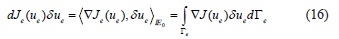
The gradient of the restriction of the functional J to the inside border of  , Ãe, Je = J|Ãe, is given by one expression of the form:
One shows now that the process by which it is obtained Equation 16 starting in Equation 14 is exactly the integration by parts method, with the border conditions appropriate for the current purpose.
Usiyng in (14) the fact that ∇J(c) = c -  , one obtains one solution c of Equation 11 and a perturbation ä of , which:
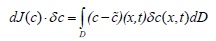
Defining
for all ä ∈ perturbation of c ∈ and such that L(c) = 0,
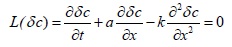
Let δ'c ∈ be. Then,
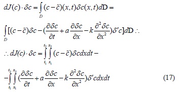
Integring by parts the terms of the second item of Equation 17, one obtains
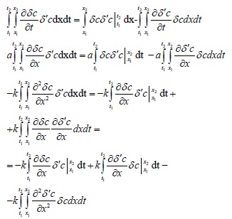
Therefore,
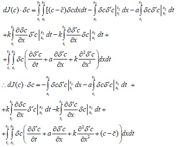
Then, by taking as solution of the non homogeneous adjoint equation,  the initial condition δ'c(t2,x) = 0, ∀x ∈[x1,x2], and the border conditions δ'c(t,x1) = δ'c(t,x2) = 0, ∀t ∈[t1,t2], one obtains:
So, the gradient de with respect to initial and border conditions, in other words, restrict to the space Ãe, is:

Therefore, in the iterative resolution, by means of a minimization routine, using the gradient of the functionl J, of problem in Equation 13,, one considers the problem:
what represents a considerable gain in the necessary computations.
4.RESULTS
4.1.Implementing the Adjoint Equation Method
Another interesting and also important feature of the implementation of Variational Data Assimilation is the development of automatic routines to perform the data assimilation using the Adjoint Equation Method. Nowadays, due to the several academic and industrial application of the method and considering the extension of the work needed to produce such computational routine, the automatic generation of the adjoint to a given code can be realized by computational codes developed for this task (Faure and Papegay, 1998). As a good knowledge of the rules used in the preparation of the linear and the adjoint programs to a given computational code precede the correct use of such automatic routines, it is presented here some illustrative examples of the rules to be followed when manually generating these codes. Of course, the rules are the same used by automatic routines.
A computational code in, exempli gratia, FORTRAN language is nothing but an ordered sequence of command lines and sometimes one or more subroutines or functions, which are also made of an ordered sequence of command lines. One begins defining a rule to obtain the adjoint instruction to a given command line, and, in the sequel, it is derived the adjoint instruction to the instruction resulting of two consecutive command lines. Let one consider the following FORTRAN command line,
Z = 2*X + Y**3,
which can be identified with the fuctio
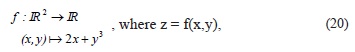
or even with the function
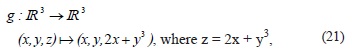
a very useful process in order to clarify the many stages in the work out of the adjoint instruction and its implementation, decreasing the possibility of errors when writing the computational code.
Although Equation 20 and Equation 21 are mathematically equivalents, notation in Equation 21 is much more convenient to write the computational codes.
As g is a nonlinear operator and nonlinear operators do not posses adjoints, when a command line is equivalent to one nonlinear operation, the first action to do is to take the linear version of the nonlinear. This can be achieved simply taking the differential of the operator, or in matricial notation, much more useful for the adjoint process, considering the jacobian matrix of the operator. In the case of function g, its jacobian is given by
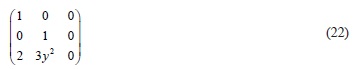
Then the linear of the instruction represented by g, dg, is:
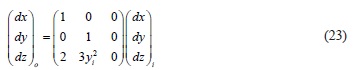
where the subscripts o and i denote, respectivelly, outside and inside amounts stored in the variables, just after and before the execution of the command line, that is,
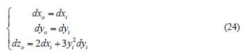
in this way, the adjoint instruction is obtained by the matrix in Equation 21:
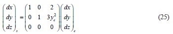
From operation in Equation 25 one obtens the adjoint instruction to the instruction in expression (19):
By associating each instruction line of one code to a funciton, therefore, this means that a program is a composition of functions. So, the linear version of the given program is obtained by using the Chain Rule of the Calculus, while the adjoint of a given code, by multipliyng the reverse order the adjoint matrices that correspond to each command line. The processes, although simple, demands careful, since one outside variável in a command line can or not be defined using the same variable (in this case, seem as na inside variable), as it will be considered later.
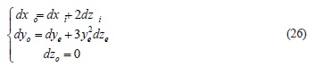
Let the instructions be:
Z = X + 2*Y
W = Y + Z**2,
Which will be refered as i1 and i2 respectively.
The following functions are associated with the previous instructions:
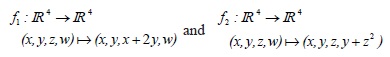
To make clearer the processes of taking the linear and the adjoint of a given instruction, as well as the writting of the correspondent instructions in FORTRAN, one adopts the following convention:
1E e → Ei e 2Ei → Es, where Ee, Ei in=1(Ei) and Es=2(Ein) are, respectivelly, the inside space, the intermediate space and the outside space, all isomorphs to 4. Then
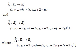
vI = (x,y,z,w) is a vector of inside data and vO = (ve), is a vector of outside data, resulting of the action of the instructions in the vector of inside data vi. Given a perturbation di of the vector of inside data, one obtains the correspondent perturbation do in the vector of outside data, in order words, d
(v) di = do, which, by the Chain Rule, it is expressed by do = d2(vin).d1(vi)di, where vin = 1 (vi) is the vector of intermediate data.
Computing ddo = d2(vin) and d1(vi), in the case vi = (x,y,z,w) ∈ Ee e vin = (x,y,x+2y,w) ∈ Ein , tem-se:
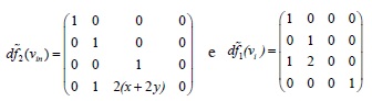
Therefore, given any direction, di= (dxi, dyi, dzi, dwi) ∈ Ee, one obtains:
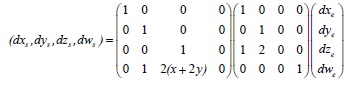
that is:
Leaving the inside and outside índexes (which are not written in a real code) and discarding the unchanged variables, as dx = dx and dy = dy, the linear instruction of instructions i1 and i2 above are the following FORTRAN instructions:
dZ = dX + 2*dY
dW = (2* X + 4* Y)* dX + (4* X + 8* Y + 1)* dY
as it was expected.
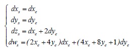
Considering that
1Ee → Ei and2Ei → Es, the adjoint to the instructions i1 and i2 are *1Ei → Ee and *1Ei → Ee,
from it follows that [d
(vs)]*(ds) = [d1(vi)]* º [d2(vs)]*(ds) = de, where:
and
Then, given ds = (dxs, dys, dzs, dws) ∈ Es, one obtains:
that is:
Considering that vs = (xe+2ye) and leaving the índices, one obtains the adjoint instruction in FORTRAN as:
dX = dX + dZ + 2* (X + 2Y)dW
dY = dY + 2* dZ + 4* (X + 2Y*)dW
And now consider the case in which one of the variables appears in one command line as an outside variable and as an inside variable. So, let i3 and i4 be the instructions:
Y = X*Y**2
Y = Y**3*X**2
To attain the necessary clarity in the development of the adjoint code, one defines the functions associated with the above instructions using the already introduced notation of inside, intermediate and outside spaces, Ee, Ei and Es, respectively, in this case, all isomorphs to 2:
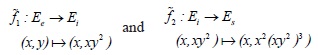
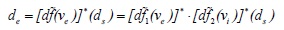
such that, to the inside vector ve = (x,y), the two instructions produce the outside vector vsgiven by:
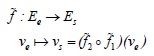
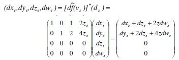
For the Chain Rule, the linear of the composition of the instructions is given by ds = d2(vi).d1(ve)de, where de is a perturbation in the inside vector, ds , and the correspondent perturbation in the outside vector is vi = 1 (ve) = (x,xy2).
Therefore, given de = (dxe, dye), one obtains
So, in FORTRAN, the linear of the commands i3 and i4 is given by:
dY = Y**2*dX + 2*X*Y*dY
Y = X*Y**2
dY = 2*X*Y**3*dX + 3*Y**2*X**2*dY
Y = Y**3*X**2
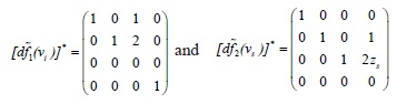
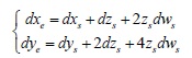
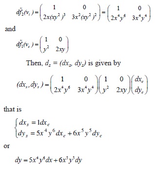
and the adjoint of the instructions is obtained from ,
where de and ds, respectively, are perturbations in the inside and outside vectors, tha is:
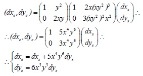
Therefore, in FORTRAN, the adjoint instructions to i3 and i4 are given by:
I0 = Y
Y = X*Y**2
I1 = Y
Y = Y**3*X**2
Y = I1
dX= dX + 2*X*Y**3*dY
dY = 3*Y**2*X**2*dY
Y = I0
dX = dX + Y**2*dY
dY = 2**Y*X*dY
4.2 Numerical experiment
One studied the oil stain trajectory determination in a region whose hydrodynamics were known and a set of oil spot observation within the time interval [t1,t2] was available. It was also supposed that all observations were incomplete, so that, at any time t1 < t < t2, the avalilable observation Z(t) can not reproduce integrally the oil spot, and, therefore, could not be used as an "initial condition" in the integration of the numerical model.
The first step of the experiment was to simulate an oil spillage in spatial domain of 6000m × 4400m, discretized by means of bidimensional grid of 21 × 21 nós, where ∆x = 300m, ∆y = 220m and the time interval of analysis was [0,30000] in seconds, with ∆t = 300s. It was taken the velocity of the medium as u = 0.1 × 10⁻¹ m/s-1 and v = 0.0, C was the concentration of oil, and D was the variable coefficient of diffusivite. The transport of the oil spot was described by the bidimensional advection-diffusion
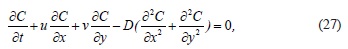
which is the universal transport model of oil in the sea surface (Lehr and Cekirge, 1980). In Figure 1, one sees the flow chart to the Data Assimilation using the Adjoint Equation Method.
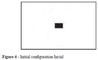
One has integrated then the Equation 27 using as initial condition the artificial oil spill (Figure 2) and, with the integration of Equation 27 (in G(U)), were storage, as system observations, the configurations obtained at the times t = 10 × i, i = 1,...9. In Figures 3 and 4, are shown the partial configurations of the oil spot for t = ∆t×20 and t = ∆t×90. One aletory perturbed the initial configuration, shown in Figure 2, by using the RAND function from the FORTRAN 90 Library, and it was obtained the perturbed initial configuration (Figure 5) , which was the begining of the Variational Data Assimilation process , and after the first integration of Equation 27, in order to generate the (toy) observations, the Equation 27 is then integrated with an initial condition obtained from the minimization routine, and the error between the model generated configurations and the observations are measured in J(G(U)). If the value measured is above the tolerance, the main program calls the subroutine D(G(U))*, in order to obtain the integration backward in time of the adjoint Equation 7, which gives the gradient of the functional J in relation to the initial conditions of the problem, which is then sent to the minimization subroutine (L-BFGS), giving a new initial configuration U which, after integration in G(U), will decrease the value of J(G(U)). When the error generated by the two configurations, model generated and observations, measured in J(G(U)), is bellow the tolerance, the process of Data Assimilation stopped, producing the optimal initial condition (Figura 6).
In the considered example, the optimal initial condition (Figura 3) was obtained, recovering the initial condition of the problem with an error less than 2%.
5.CONCLUSIONS
Data Assimilation, process in which observations of the studied systems are considered as conditions to the computational simulation must verify, together with Adjoint Equation Method, produce a methodology to obtain reliable and highly accurate computational configurations of a system at a feasible computational cost and within a time interval that allows na effective decision in an oil spill.
A further question, also in the realm of the formalism presented here, is the optimal location of measurement instruments, enhancing an existing network.
6. REFERENCES
Received September
Accepted January 2011
- DALEY, R. Atmospheric Data Analysis, Cambridge University Press, 472, 1993.
- ELBERN, H., STRUNK, A., SCHIMDT, H., TALAGRAND, O. Emission rate and chemical state estimation by 4-dimensional variational inversion, Atmos. Chem. Phys7, 3749-69, 2007.
- FAURE, C., PAPEGAY, Y. Odyssée User's Guide, Version 1.7, INRIA, 1998.
- GIERING, R., KAMINSKI, T., TODLING, R., ERRICO, R., GELARO, R., WINSLOW, N. Generating tangent linear and adjoint versions of NASA/GMAO's Fortran-90 global weather forecast model. In H.M. Bücker, G. Corliss, P. Hovland, U. Naumann, and B.Norris, editors, Automatic Differentiation: Applications, Theory, and Implementations, Lecture Notes in Computational Science and Engineering, v. 50, pages 275-284. Springer, New York, NY, 2005.
- KALNAY, E. Atmospheric Modeling, Data Assimilation and Predictability, Cambridge University Press, 364, 2002.
- KAMIEN, M.I., SCHWARTZ, N.L. Dynamic optimization: the calculus of variation and optimal control in economics and management, North-Holland, 1981.
- KAMINSKI,T., GIERING, R., SCHOLZE, M., RAYNER, P., KNORR, W. An example of an automatic differentiation-based on modelling system, Conference proceeding, Computational Science and Its Applications ICCSA 2003, Proceedings of the International Conference on Computational Science and its Applications, Montreal, Canada, May 18--21, 2003. Part II, Springer, 2003.
- KREYSZIG, E.; Introductory Functional Analysis with Applications, John Wiley and Sons, 1989.
- LE DIMET, F. X., TALAGRAND, O. Variational algorithms for analysis and assimilation of meteorological observations: theoretical aspects, Tellus, 38A, 1986.
- LEHR, W.J., CEKIRGE, H. M. Oil slick movements in the Arabian Golf, Proceeds of Petroleum and Marine Environment, Monaco, 1980.
- LIONS, J.L. Optimal Control of Systems Governed by Partial Differential Equations, Springer - Verlag, 1971.
- LIU, D., NOCEDAL, D. On the limited memory BFGS method for large scale minimization, Mathematical Programming, 45, pp.: 503-528, 1989.
- LORENZ, E.N.; Deterministic non-periodic flows, Journal of Atmospheric Sciences, 20, pp.: 130-141, 1963.
- PARRISH, D.F., DERBER., J.D. The national meteorological center spectral statistical interpolation analysis system. Mon. Wea. Rev, 120:1747-1763, 1992.
- REUTHER, J., JAMESON, A., FARMER, J., MARTINELLI, L., SAUNDERS, D. Aerodynamic shape optimization of complex aircraft configurations via an adjoint formulation, AIAA Journal , 96-0094, 1996.
- SORENSEN, H.W.; Parameter estimation: principles and problems, Marcel Dekker, 1980.
- TALAGRAND, O.; Assimilation of observations, an introduction, Journal of Meteorological Society of Japan, v. 75, n. 1B, pp.: 191-209, 1997.
- TALAGRAND; .A study of the dynamics of four-dimensional data assimilation, Tellus, 33, 43-60, 1986.
- THOMAS, J. P., HALL, K. C. Sensitivity analysis of coupled aerodynamic/structural dynamic behavior of blade rows. Extended Abstract for the 7th National Turbine Engine High Cycle Fatigue (HCF) Conference, Palm Beach Gardens, Florida, 14-17 May 2002.
- THOMAS, J. P., HALL, K. C., DOWELL, E.H. A discrete adjoint approach for modeling unsteady aerodynamic design sensitivities. AIAA Journal., 43(9):1931-1936, 2005.
Publication Dates
-
Publication in this collection
11 Nov 2011 -
Date of issue
Sept 2011
History
-
Received
Sept 2011 -
Accepted
Jan 2011