Precipitation trends analysis by Mann-Kendall test: a case study of Paraíba, Brazil

Análise de tendência da precipitação usando o teste de Mann-Kendall: um estudo de caso na Paraíba, Brasil

Abstract

This work aimed to select semivariogram models to estimate trends in monthly precipitation in Paraiba State-Brazil using ordinary kriging. The methodology involves the application of geostatistical interpolation of precipitation records of 51 years from 69 rainfall stations across the state. Analysis of semivariograms showed that specific months had a strong spatial dependence (Index of Spatial Dependence - IDE < 25%). The trends were subjected to the following models: circular, spherical, pentaspherical, exponential, Gaussian, rational quadratic, K-Bessel and tetraspherical. The best fit models were selected by cross-validation and Error Comparison Index (ECI). Each data set (month) had a particular spatial dependence structure, which made it necessary to define specific models of semivariogram in order to enhance the adjustment of the experimental semivariogram. Besides, the monthly trend map was plotted to justify the chosen models.

Keywords:
precipitation; trends; Paraíba; geostatistics

Resumo

Este trabalho teve como objetivo selecionar modelos de semivariograma para estimar tendências de precipitação mensal no Estado da Paraíba-Brasil usando krigagem comum. A metodologia envolve a aplicação de interpolação geoestatística de registros de precipitação de 51 anos de 69 estações de chuva em todo o estado. A análise de semivariogramas mostrou que meses específicos apresentaram forte dependência espacial (Índice de Dependência Espacial - IDE <25%). As tendências foram submetidas aos seguintes modelos: circular, esférico, pentassesférico, exponencial, gaussiano, quadrático racional, K - Bessel e tetrasspherical. Os melhores modelos de ajuste foram selecionados por validação cruzada e Índice de Comparação de Erros (ICE). Cada conjunto de dados (mês) possuía uma estrutura de dependência espacial específica, o que tornava necessário definir modelos específicos de semivariograma, a fim de aprimorar o ajuste do semivariograma experimental. Além disso, o mapa mensal de tendências foi plotado para justificar os modelos escolhidos.

Palavras-chave:
precipitação; tendências; Paraíba; geoestatística

1. Introduction

Northern South America distinguishes by being a large and complex region where distinct weather systems act. According to Andreoli et al. (2012), the Amazon region, which represents one of the most intense convective areas in the world, and northeast of Brazil, which is related to intense and prolonged droughts due to its semi-arid climate, are inserted in northern South America. The cooperation between different atmospheric phenomena that appear in the whole region and local surface conditions (like vegetation, topography, and land use), generates a non-homogenous rainfall distribution that exhibits in a broad temporal and spatial range (Sierra et al., 2015).

Rainfall is a periodical spatiotemporal phenomenon displaying significant spatial and temporal variability, and rain gauge networks only collect point estimates. Therefore, providing an estimate of spatial rainfall distribution within an area from rain gauge data usually remains a barrier of interpolation (Mirás-Avalos et al., 2007).

Rainfall data is an essential input for hydrological systems; this type of information plays a fundamental role in understanding the hydrological cycle. An accurate estimation of precipitation is crucial. In developing countries, the availability of rainfall data is obstructed by the scarcity of precise, high-resolution precipitation. Since its inception, rainfall measurement principles have remained unchanged; non-recording and recording rain gauges are still the standard equipment for measuring ground-based precipitation, notwithstanding that they only provide point measurements. According to Ochoa et al. (2014), rainfall amounts evaluated at different locations are usually extrapolated to obtain areal-average rainfall estimates.

Understanding the variability of precipitation regime over tropical South America is crucial because of the strong dependence of water supply, hydro-energy, agriculture, and transportation. Brazilian agriculture is principally supported by natural irrigation. Hence, the importance of understanding the mechanism to produce water through precipitation variability in tropical South America has not only meteorological implications but also practical applications for the society in the region.

As reported by Zhou and Lau (2001) and Takahashi (2004), precipitation variability in South America has been influenced by particular factors such as Atlantic Sea Surface Temperature (SST), El Niño-Southern Oscillation (ENSO), and Intertropical Convergence Zone (ITCZ). Grimm (2011) also considered that the ENSO impact on the characteristics of Brazil Northeast precipitation is related to the position of ITCZ and Atlantic and Pacific SST interaction.

Geostatistics based on the theory of regionalized variables permits the analysis and interpretation of any spatially (temporally) referenced data (Isah, 2009). It is increasingly preferred because it capitalizes on the spatial correlation between neighboring observations to predict attribute values at unsampled locations (Goovaerts, 2000). Several studies (Creutin and Obled, 1982; Tabios and Salas, 1985; Lebel et al., 1987 and Goovaerts, 2000) have demonstrated that the estimation of precipitation by appropriate geostatistical tools permits more accurate results than other forms of interpolation. The possibility of quantifying uncertainty for an interpolated point or area is particularly useful, as it allows more meaningful comparison with rainfall estimates generated by other means (e.g., radar, satellite, or numerical weather models). It also facilitates the investigation of the propagation of uncertainty in downstream models (e.g., hydrological or agricultural forecast models). However, interpretation of the kriging variance as an estimate of error depends on the data obeying the implicit statistical assumptions of kriging, but some caution may be needed.

Hence, the evaluation of historical trends or future projections on a regional or local scale is necessary. This study is therefore intended to investigate trends in the monthly precipitation series in the State of Paraíba, Brazil, and to determine whether there have been any significant changes in precipitation trends from 1962 to 2012. It was used spatial clustering analysis to identify spatial explicit and statistically significant rainfall stations. Such an integrated spatiotemporal analysis facilitates a spatial quantification of potential precipitation vulnerability hot spots.

2. Material and Methods

2.1. Data

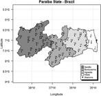
The study was carried out in Paraiba state, located in the Brazilian Northeast, as shown in Fig. 1. The Brazil Northeast has 1.5 × 10⁶ km² of the area ranging between 1-18 °S and 35-47 °W; different meteorological systems influence the region with distinct characteristics (Filho et al. 2014). As stated in Liebmann et al. (2011), Kouadio et al. (2012), in Northeast extreme events, are related to deficit precipitation (semiarid region) or excess precipitation (capitals or Coast regions). Nevertheless, the amount of precipitation in Paraiba is related to various meteorological systems: Intertropical Convergence Zone (ITCZ), High-Level Cyclone Vortex (HLCV), Jet Streams. According to Macedo et al. (2010), Paraiba is one of the Brazilian states which presents an evident water scarcity, as it has a semi-arid climate in most of its territory. The data required for calculation of trends were obtained for a total of 69 precipitation stations having a typical period from 1962 to 2012. The data were collected from Instituto Nacional de Meteorologia (INMET) and acquired by Unidade Acadêmica de Ciências Atmosféricas (UACA-UFCG). According to De Amorim Borges et al. (2014), it is crucial to have access to reliable data, which are free from artificial trends or changes. The following are the procedures for data quality control. The first step was assembling available data and selecting the candidate station series for trend analysis based on the series length and data completeness. The second step was the visual checks of data plots, which reveal outliers as well as a variety of problems that cause changes in the variance of the data or the seasonal cycle. Thereon, rainfall gauges presented a homogeneous spatial distribution around the state and included all micro-regions of Paraiba state. The spatial locations of the stations chosen are shown in Fig. 1.

Figure 1
Spatial distribution of 69 precipitation stations used in the study.

2.2. Methodology

2.2.1. Mann-Kendall Test

The Mann-Kendall test had been formulated by Mann (1945) as a non-parametric test for trend detection, and the statistical distribution of test had been given by Kendal (1975) for evaluating non-linear trend and the change point. The test has been extensively used to detect trends and spatial variation in hydroclimatic series, that is, meteorological, hydrological, and agro-meteorological time series. Many authors (Dias et al., 2013 and Sayemuzzaman and Jha, 2014) have used this test to evaluate the presence of significant climate trends in different parts of the world.

A factor that affects trend detection in a series is the presence of positive or negative autocorrelation (Yue et al. 2003; Novotny and Stefan, 2007). A positive autocorrelation does not guarantee a series of being detected as having a trend. By contrast, for negative autocorrelation, this is inverse, where the trend is not detected. ${\rho }_k$, the autocorrelation coefficient of a discrete-time series for lag-k, can be expressed as

(1) $${\rho }_k=\frac{{\sum }_{k=1}^{n-k}\left(x_t-{\overline{x}}_t\right)\left(x_{t+k}-{\overline{x}}_{t+k}\right)}{{{\sum }_{t=1}^{n-k}{\left(x_t-{\overline{x}}_t\right)}^2*{\sum }_{n-k}^{t=1}\left(x_{t+k}-{\overline{x}}_{t+k}\right)}^2}$$

where, ${\overline{x}}_t$ and $Var\left({\overline{x}}_t\right)$ are the sample mean and sample variance of the first $\left(n-k\right)$ terms, respectively, and ${\overline{x}}_{t+k}$ and $Var\left({\overline{x}}_{t+k}\right)$ are the sample mean and the sample variance of the last $\left(n-k\right)$ terms, respectively. Besides, the hypothesis of serial independence is tested by the lag-1 autocorrelation coefficient as $H_0:{\rho }_1=0\times H_1:\left|{\rho }_1\right|\ne 0$ using the following statistic

(2) $$t=\left|\rho \right|\sqrt{\frac{n-2}{1-{\rho }^2}}$$

where the statistic of the test has a Student’s t-distribution with $\left(n-2\right)$ degrees of freedom. If occurs that $\left|t\right|>t_{\frac{\alpha }{2}}$, so the null hypothesis is rejected at the chosen significance level $\alpha$.

The computational method for the Mann-Kendall test considers the time series for n data points $R_i$ and $R_j$ as two subsets of data where $i=1,2,\dots ,n-1$ and $j=i+1,i+2,\dots ,n$. The data values are measured as an ordered time series. Thus, each data value is compared with all subsequent data values. If it occurs that a data value from a later period is higher than a data value from an earlier period, statistic S is incremented by 1. Further, if the data value from a later period is lower than a data value from a previous period, statistic S is decremented by 1. The net result of all such increments yields the final value of S.

Given a time series $X=x_1,\dots ,x_n$ that is ranked from $R_i=R_1,\dots ,R_n$ the statistic S is calculated as

(3) $$S={\displaystyle \sum {}_{i<j}^{}sgn\left(R_j-R_i\right)}$$

each data point $x_i$ is taken as a reference point which is compared with the rest of the data points $x_j$ such as

(4) $$Z_i=sgn\left(x_j-x_i\right)=\{\begin{array}{c}+1,if{x}_j>x_i\\ 0,if{x}_j=x_i\\ -1,if{x}_j<x_i\end{array}$$

Mann (1945) reported that when $n<8$ statistic S is approximately normally distributed with $E\left(S\right)=0$. The variance is given as

(5) $$Var\left(S\right)=\frac{1}{18}\left[n\left(n-1\right)\left(2n+5\right)-{\sum }_{i=1}^m{t}_i\left(i\right)\left(i-1\right)\left(2i+5\right)\right]$$

wherein $t_i$ is considered as the number of ties up of sample i, and the summation is overall ties. The standardized normal test statistic is calculated as

(6) $$Z\left(n\right)=\frac{S}{{\left[Var\left(S\right)\right]}^{1/2}}$$

Test statistics $Z_c$ is computed as

(7) $$Z_c=\{\begin{array}{c}\frac{S-1}{\sqrt{Var\left(S\right)}},ifS>0\\ 0,ifS=0\\ \frac{S+1}{\sqrt{Var\left(S\right)}},ifS<0\end{array}$$

$Z_c$ has a standard normal distribution. A positive value of $Z_c$ implies an ascendant value of trend and vice-versa. A significant level $\alpha$ is also utilized for testing either an ascendant or descendant monotone trend, that is, a two-tailed test. If $Z_c>Z_{\frac{\alpha }{2}}$, where $\alpha$ states the significant level, so the trend is considered as significant.

2.2.2. Geostatistical techniques

Geostatistics has been defined by Matheron (1963) as “the application of probabilistic methods to regionalized variables,” which designates any function displayed in real space. Different from conventional statistics, whatever the complexity and the irregularity of the real phenomenon, geostatistics searches to exhibit a structure of spatial correlation. Geostatistical methods use semivariograms as a core tool to characterize the spatial dependence in the property of interest (Ly et al., 2011). Geostatistics uses the concept of random functions to build a model for physical reality, bringing up these two contradictory characteristics random and structured. As reported by Heuvelink et al. (1997), its necessary apparatus is variogram analysis, which contains the study of the variogram function of a specific physical variable value or a water quality parameter under study.

2.2.2.1. Kriging

Kriging is the term used by geostatisticians for a family of generalized least-squares regression methods that use available data in a specific search neighborhood to estimate the values at unsampled locations (Isaaks, 1989; Goovaerts, 1997). As stated in Berke (1999), it is based on a linear spatial model for the data which specify a parametric spatial mean function and spatial dependence structure. As stated by Isaaks (1989), kriging uses a variogram model to characterize spatial correlation. A variogram describes concerning variance how spatial variability changes as a function of distance and direction. Kriging uses statistical models and allows a variety of map outputs, including predictions, prediction standard errors, probability, among others. Today, some variants of kriging are in general use, such as Simple Kriging, Ordinary Kriging, Block Kriging, Universal Kriging, Co-Kriging, and Disjunctive Kriging. Amidst the various forms of kriging, Ordinary Kriging has been used extensively as a reliable estimation method (Yamamoto, 2000). In short, Ordinary Kriging is the primary form of kriging. It has been widely used with rainfall data. Ordinary Kriging prediction is a linear combination of measured values.

2.2.2.2. Semivariogram

Semivariogram is a convenient tool for the analysis of the spatial dependence structure (Cressie, 1993). If the spatial dependence exists, its degree is quantified by comparing the models to the experimental semivariogram. Using Eq. 8 to compute experimental semivariogram from the data under study is the only guaranteed way to describe how semivariance changes with distance, determine which semivariogram model should be used. By changing, both in distance and direction, a set of the sample (or experimental) semivariograms for the data is obtained (Burrough, 1986).

(8) $$\gamma \left(h\right)=\frac{1}{2N\left(h\right)}={\displaystyle {\sum }_{i=1}^{N\left(h\right)}\left[Z(X_i\right)-Z\left(X_i+h\right){]}^2}$$

where $\gamma \left(h\right)$ is the semivariance as well as $N\left(h\right)$ is the number of $Z\left(X_i\right)$ and $Z\left(X_i+h\right)$, separated by a h vector.

A variety of theoretical models can be utilized to adjust from the experimental semivariogram to the theoretical semivariogram. Notwithstanding, Johnston et al. (2001) showed 11 theoretical models, such as Spherical, Exponential, Gaussian, Linear, Circular, Tetraspherical, Pentaspherical, Rational Quadratic, Hole Effect, K-Bessel, and J-Bessel.

Applying the algorithm of weighted least squares (WLS), these models were adjusted to the experimental semivariogram, and the subsequent model parameters were defined: nugget effect ${\sigma }^2$, sill ${\tau }^2+{\sigma }^2$, and range $\varphi$. In order to verify the existence of spatial dependence, the spatial dependence index (SDI), proposed by Cambardella et al. (1994), was applied, which is the ratio representing the percentage of data variability explained by spatial dependence.

The SDI is estimated as follows: $\text{SDI}=\left[{\tau }^2/{\tau }^2+{\sigma }^2\right]100$ being classified as strong $\left(\text{SDI}\le 25\%\right)$, medium (25 < SDI < 75%), and low (SDI ≥ 75%).

2.2.2.3. Cross-validation

Goovaerts (1997) explains that cross-validation allows comparing the impact of interpolators among the real estimated values, in which the model with more accurate prediction is chosen. Cross-validation allows the determination of models that provide the best prediction (Johnston et al., 2001). The semivariogram model was selected in consonance with the cross-validation technique (Webster and Oliver, 2007). Faraco et al. (2008) recognized the cross-validation criterion as the most adequate for choosing the best semivariogram adjustment. The semivariogram models were verified for each parameter data set. The quality of prediction performances is assessed by cross-validation. Cross-validation was conducted to evaluate the accuracy of Ordinary Kriging through some statistical measurements as follows:

• i) Mean Prediction Errors,

  (9)$$ME={\sum }_{i=1}^n\frac{\left[\widehat{Z_{(t_{i)}}}-Z_{\left(t_i\right)}\right]}{n}$$

• ii) Mean Standardized Prediction Errors,

  (10)$$MS=\frac{{\sum }_{i=1}^n\frac{\left[\widehat{Z_{(t_{i)}}}-Z_{\left(t_i\right)}\right]}{\widehat{{\sigma }_{t_i}}}}{n}$$

• iii) Root Mean Square Error,

  (11)$$\text{RMSE}=\sqrt{{\sum }_{i=1}^n\frac{\left[\widehat{Z_{(t_{i)}}}-Z_{\left(t_i\right)}\right]²}{n}}$$

• iv) Average Standardized Error,

  (12)$$AE=\sqrt{\frac{{\sum }_{i=1}^n\widehat{{\sigma }_{t_i}}}{n}}$$

• v) Root Mean Square Standardized Error,

  (13)$$RMSSE=\sqrt{\frac{{\sum }_{i=1}^n\frac{\left[\widehat{Z_{(t_{i)}}}-Z_{\left(t_i\right)}\right]}{\widehat{{\sigma }_{t_i}}}}{n}}$$

According to Johnston et al. (2001), to evaluate a model that provides accurate predictions, the standardized average (MS) should be close to 0, the square root of standardized mean error (RMSSE) should be close to 1. The average standard error (ASE) and the root mean square error (RMSE) and should be as small as possible. In order to verify the best choice among J different fitted models and their MS values close to 0 and RMSSE values close to 1. Santos et al. (2012) suggested Error Comparison Index (ECI), which can be calculated as follows:

(14) $$EC{I}_i=A_i+B_i$$

where,

(15) $$A_i=\{\begin{array}{ccc}& \frac{ABS{\left(MS\right)}_i}{MAX(ABS(MS\left)\right)},& whenMAX\left(ABS\left(MS\right)\right)>0\\ 1,& whenMAX\left(ABS\left(MS\right)\right)=0& \end{array}$$

(16) $$B_i=\{\begin{array}{ccc}& \frac{ABS{\left(RMSS-1\right)}_i}{MAX\left(ABS\left(MS\right)\right)},& whenMAX\left(ABS\left(RMSS-1\right)\right)>0\\ 1,& whenMAX\left(ABS\left(RMSS-1\right)\right)=0& \end{array}$$

The best-fitted model among J different models is one that presents the lowest ECI value.

3. Results and Discussion

In this section, we present trend analysis results for monthly precipitation. To choose the best-fitted model that would predict the trend of precipitation in Paraiba, we used cross-validation. The cross-validation that examines the validity of fitted models and parameters of semivariograms for precipitation parameters are given in Table 1. Data analysis and Mann-Kendall test, spatial trends, experimental semivariograms, and geostatistical analysis were done by using the R Development Core Team (Team, 2013).

Table 1
Values of ME, RMS, MS, RMSS, ASE, spatial dependence index (SDI), and error comparison index (ECI) for trends of precipitation between January-December.

Month	Model	ME	RMS	MS	RMSS	ASE	SDI	ECI
Jan	Spherical	0.0034	0.9410	0.0038	0.9991	0.950	41.29	0.1624
	Circular	–0.0022	0.9369	–0.0011	0.9990	0.946	42.79	0.005
	R. Quadratic	0.0116	0.9530	0.0069	0.9813	0.980	39.95	0.4986
Feb	Pentasph.	–0.0146	0.9536	–0.0114	1.0250	0.920	34.08	0.6012
	Spherical	–0.0148	0.9573	–0.0093	1.0391	0.912	43.24	0.8033
	Tetraspherical	–0.0184	0.9555	–0.0143	1.0317	0.917	39.07	0.7599
Mar	Gaussian	–0.0013	1.2012	0.0037	0.9998	1.199	53.49	0.1528
	Spherical	–0.0075	1.1362	–0.0003	0.9774	1.165	38.21	0.4617
	Tetraspherical	–0.0076	1.1172	0.0001	0.9786	1.147	33.33	0.4284
Apr	Gaussian	–0.0600	1.2102	–0.0417	0.9903	1.228	48.03	1.0453
	Spherical	–0.0491	1.2082	–0.0344	0.9924	1.223	27.40	0.8578
	Tetrasph.	–0.0327	1.2097	–0.0227	0.9977	1.219	16.80	0.5380
May	K-Bessel	–0.0159	0.9927	–0.0086	1.0011	0.986	0	0.2343
	J-Bessel	–0.0163	0.9995	–0.0124	1.0066	1.005	0	0.4049
	Tetraspherical	–0.0417	1.0229	–0.0308	1.0445	0.979	2.727	1.3732
Jun	Rat. Quadratic	–0.0082	2.0497	–0.0042	1.0248	1.978	26.36	0.3872
	K-Bessel	0.0025	2.0516	0.0014	1.1007	1.831	30.17	0.8972
	Pentaspherical	0.0106	2.0539	0.0054	1.0550	1.921	22.30	0.6894
Jul	Spherical	–0.0261	0.9658	–0.0214	0.9832	0.988	52.34	0.8500
	Circular	–0.0349	0.9628	–0.0298	0.9889	0.978	52.33	1.0150
	Pentasph.	–0.0186	0.9664	–0.0144	0.9686	1.004	53.08	0.8411
Aug	Gaussian	–0.0021	1.3396	–0.0003	1.0479	1.275	60.01	0.6077
	Exponential	0.0112	1.2936	0.0087	1.0437	1.236	31.59	1.2178
	Spherical	0.0062	1.3228	0.0055	1.0558	1.250	50.11	1.1135
Sep	J-Bessel	0.0043	1.1225	0.0037	1.0547	1.065	51.11	1.0730
	Rat. Quadratic	0.0133	1.1327	0.0104	1.0763	1.053	36.05	1.9935
	Tetrasph.	–0.0032	1.1208	–0.0028	1.0407	1.078	39.34	0.8071
Oct	Gaussian	–0.0241	1.4932	–0.0143	1.0717	1.391	46.52	1.4122
	Exponential	–0.0269	1.5077	–0.0141	0.9919	1.524	67.31	0.6617
	Spherical	–0.0283	1.5061	–0.0158	1.0514	1.437	53.15	1.2344
Nov	Exponential	–0.0054	1.0956	–0.0040	1.0416	1.047	51.55	1.1176
	Spherical	0.0004	1.0790	0.0024	1.0323	1.043	62.67	0.8031
	Circular	–0.0049	1.0825	–0.0023	1.0367	1.041	63.86	0.8792
Dec	Circular	0.0311	1.1372	0.0206	1.0749	1.039	36.77	1.4780
	Rat. Quadratic	0.0254	1.1339	0.0184	1.0071	1.110	55.33	0.7735
	Hole Effect	0.0349	1.1146	0.0216	1.1086	0.996	41.18	1.8271

According to Owolawi and Afullo (2007), Sana et al. (2014), the RMS statistic is widely used to select a semivariogram model or an implementation method. Along with RMS, the ASE statistic is used to validate statistical models. Therefore, the knowledge of obtaining the lowest ASE value and closest statistic RMS benefits in choosing the best model. On the verification by RMSS, MS, ASE and RMS statistics may generate a small distraction; we used the Error Comparison Index (ECI) suggested by Santos et al. (2012) because it helps compare the statistics used in cross-validation process and chose the best geostatistical model by the lowest ECI value. One can note from Table 1 that the model selection, which presents the best semivariogram fit, may include all errors of prognosis in an integrated manner.

Before selecting the proper spatial model, it was necessary to choose the purpose of it. Furthermore, the characteristics of the rainfall phenomenon must be analyzed, and the assumptions of the technique. The rainfall amounts over Paraíba are significantly influenced by seasonality, geographical position, and topography. The monthly rainfall maps illustrated that the spatial distribution of the rainfall is reasonably heterogenic over each month analyzed. The different models chosen by each month demonstrated the high spatiotemporal variability of the rainfall in Paraíba. The variogram’s choice was due to the statistical criterion described in the methodology and presented in Table 1.

As stated in Ly et al. (2013), the successful performance of a method depends on various components, in particular, temporal and spatial resolutions of data and parameters of the model, such as the semi-variogram in the case of kriging. Figure 2 shows the trend interpolation map for January-April adjusted according to ECI results shown in Table 1. Carvalho et al. (2004) emphasized the influence of the South Atlantic Convergence Zone (SCAZ) over the maximum values of precipitation in the Northeast of Brazil. The intraseasonal anomalies in precipitation are related to anomalies of the Pacific Ocean.

Figure 2
Spatial variation of monthly rainfall trends (mm/month) for Paraiba from 1962 to 2012 (January-April).

In March, it is conceivable that there is a considerable concentration of trends between Borborema and Agreste and not so significant in the North of Mata. This is related to the end of the rainy season between January and February. In April, the interpolation map shows increasing trends in the North and West of Sertão, as well as trends in the North and South of Mata with significant influence over the coast. In the study of Rodrigues et al. (2011), it was verified, regarding seasonal rainfall distribution, that increasing trends take place during March, April and May (autumn in South Hemisphere) caused by the influence of El Niño and La Niña phenomena.

Figure 3 displays the trend interpolation map for May-August for Paraíba. Rodrigues et al. (2011) observed negative trend intensity during June, July and August, not the periods of extreme events. In July, there was a concentration of an increasing trend almost in the entire region further west of Sertão, and large displacement in the southernmost of Borborema. Another movement of trends can be visualized from the North of Agreste through North and South of Mata addressing the coast. In August, there was a considerable concentration of the increase of trends in the South Central Borborema region with a sensible movement to the Agreste region.

Figure 3
Spatial variation of monthly rainfall trends (mm/month) for Paraiba from 1962 to 2012 (May-August).

Figure 4 shows the trend interpolation map for September-December. In October, for the first time, there was a predominance of increasing trends in the entire range of Paraíba, that is, much of Sertão, Borborema, and North of Agreste region. This predominance was also described by Gomes et al. (2014), who detailed the displacement of precipitation associated with various meteorological system activities, such as ICTZ, cold fronts. As stated in Uvo et al. (1998), when the ITCZ stays longer in the south, heavy rains occur in the northeast of Brazil, but when it does not reach its most southern position (relatively to the northeast) droughts appears in the northeast of Brazil. The anomalies in the ITCZ shifts are mainly produced by variations in the SST interhemispheric gradient in the Atlantic Ocean.

Figure 4
Spatial variation of monthly rainfall trends (mm/month) for Paraiba from 1962 to 2012 (September-December).

The mixed existence of positive and negative trends, along with the differences in the results referring to the specifically observed time interval, does not allow conclusions to be drawn of a general tendency for the investigated large-scale area. The illustrated analysis describes the observational evidence of potential dynamics in cumulative, monthly precipitation, and they have been applied at the point scale to each selected gauged site.

Boulanger et al. (2005) focused their study on the understanding of the long-term trends of precipitation through monthly data analyzing how ENSO has influenced the region. The study showed that the trend is characterized by spatial patterns that differ from month to month. The trends presented a monthly dependence with its spatial characteristics. According to Barros et al. (2008), it was not possible to consider ENSO events separately to calculate annual or seasonal trends directly. Hence, the authors evaluated linear trends of precipitation for every month of each ENSO event. The magnitude of the trends was large, positive and statistically significant over the studied area.

Liu et al. (2016) studied the magnitude and trends in precipitation in response to global warming in order to identify the primary controlling mechanisms of the trends. The magnitude of the trends was displayed through regional maps of precipitation. The authors identified that the increasing trend of one month is the key contributor to the increasing trend of regional annual precipitation in the study area. Wilby and Dawson (2013) showed that regional climate models are often required to understand the climate information through water resources management is of a spatial scale much finer than that provided by global models.

4. Conclusions

In this paper, we analyze rainfall trends over the entire Paraíba state, where significant changes in rainfall trends have occurred during all months. It is noticeable that rainfall trends vary across the state for many reasons (e.g., topography, forest cover, ITCZ, distance from the coast, among others) The impact of possible changes in rainfall trend intensity adds complexity to the implications of our results. Average rainfall trend levels may vary slightly, but if rain falls only at one time in the seasonal calendar or too late or too early in the agricultural cycle, then everything which is related may suffer.

For a better understanding of trends, monthly rainfall trend maps have been generated by following a methodology that includes geostatistical techniques. Geostatistical algorithms were applied to estimate rainfall trend patterns from data recorded at 69 rainfall stations distributed across the state. The analysis for all rainfall stations reveals increasing (decreasing) trends that, associated with public policies, facilitate an overview of the scarcity of resources to understand the rainfall phenomenon and the low rainfall level during the drought period, which affects most parts of the State.

It is worthwhile emphasizing that the trend results presented in this study were not sufficient to approve a climatic change in Paraiba. Future studies are needed to address the issue of trend attribution and to attempt to establish a linkage between climate change and observed hydrologic trends.

Acknowledgments

The authors are grateful to the CNPq for funding the Research Project nº 446172/2015-4 and the Research Productivity Grant (Grant N. 304493/2019-8) for the fourth author, as well as the CAPES for funding the Research Project nº 88887.091737/2014-01.

References

• ANDREOLI, R.V.; SOUZA, R.A.F.; KAYANO, M.T.; CANDIDO, L.A. Seasonal anomalous rainfall in the central and eastern Amazon and associated anomalous oceanic and atmospheric patterns. International Journal of Climatology, v. 32, n. 8, p. 1193-1205, 2012.
• BARROS, V.R.; DOYLE, M.E.; CAMILLONI, I.A. Precipitation trends in southeastern South America: relationship with ENSO phases and with low-level circulation. Theoretical and Applied Climatology, v. 93, n. 1-2, p. 19-33, 2008.
• BERKE, O.I. Estimation and prediction in the spatial linear model. Water, Air and Soil Pollution, v. 110, n. 3-4, p. 215-237, 1999.
• BOULANGER, J.P.; LELOUP, J.; PENALBA, O.; RUSTICUCCI, M.; LAFON, F.; VARGAS, W. Observed precipitation in the Paraná-Plata hydrological basin: Long-term trends, extreme conditions and ENSO teleconnections. Climate Dynamics, v. 24, n. 4, p. 393-413, 2005.
• BURROUGH, P.A. Principles of geographical information systems for land resources assessment. Geocarto International, v. 1, n. 3, p. 54-54, 1986.
• CAMBARDELLA, C.A.; MOORMAN, T.B.; PARKIN, T.B.; KARLEN, D.L.; NOVAK, J.M.; TURCO, R.F.; KONOPKA, A.E. Field-scale variability of soil properties in central Iowa soils. Soil Science Society of America Journal, v. 58, n. 5, p. 1501-1511, 1994.
• CARVALHO, L.M.; JONES, C.; LIEBMANN, B. The South Atlantic convergence zone: intensity, form, persistence, and relationships with intraseasonal to interannual activity and extreme rainfall. Journal of Climate, v. 17, n. 1, p. 88-108, 2004.
• CRESSIE, N.A. Statistics for Spatial Data: Revised Edition John Wiley & Sons, Michigan, USA, 1993.
• CREUTIN, J.D.; OBLED, C. Objective analyses and mapping techniques for rainfall fields: an objective comparison. Water Resources Research, v.18, n. 2, p. 413-431, 1982.
• De AMORIM BORGES, P.; FRANKE, J.; dos SANTOS SILVA, F.D.; WEISS, H.; BERNHOFER, C. Differences between two climatological periods (2001-2010 vs. 1971-2000) and trend analysis of temperature and precipitation in Central Brazil. Theoretical and Applied Climatology, v. 116, n. 1-2, p. 191-202, 2014.
• DIAS, M.A.S.; DIAS, J.; CARVALHO, L.M.; FREITAS, E.D.; DIAS, P.L.S. Changes in extreme daily rainfall for São Paulo, Brazil. Climatic Change, v. 116, n. 3-4, p. 705-722, 2013.
• FARACO, M.A.; URIBE-OPAZO, M.A.; SILVA, E.A.A.D.; JOHANN, J.A.; BORSSOI, J.A. Selection criteria of spatial variability models used in thematical maps of soil physical attributes and soybean yield. Revista Brasileira de Ciência do Solo, v. 32, n. 2, p. 463-476, 2008.
• GOMES, O.M.; MOREIRA, G.R.; de OLINDA, R.A.; SANTOS, C.A.C. Análise de superfície de tendência aplicada a dados de precipitação pluvial do estado da Paraíba. Revista Brasileira de Biometria, v. 32, n. 3, p. 412-429, 2014.
• GOOVAERTS, P. Geostatistical approaches for incorporating elevation into the spatial interpolation of rainfall. Journal of Hydrology, v. 228, n. 1-2, p. 113-129, 2000.
• GOOVAERTS, P. Geostatistics for Natural Resources Evaluation Oxford University Press, New York, 1997.
• GRIMM, A.M. Interannual climate variability in South America: Impacts on seasonal precipitation, extreme events, and possible effects of climate change. Stochastic Environmental Research and Risk Assessment, v. 25, n. 4, p. 537-554, 2011.
• HEUVELINK, G.B.M.; MUSTERS, P.; PEBESMA, E.J. Spatio-temporal kriging of soil water content Kluwer Academic Publishing., Dordrecht, Netherlands, 1997.
• ISAAKS, E.H.; SRIVASTAVA, R.M. An Introduction to Applied Geostatistics Oxford University, New York, 1989.
• ISAH, A. Spatio-temporal modeling of nonstationary processes. Journal of Science, Education and Technology, v. 2, n. 1, p. 372-377, 2009.
• JOHNSTON, K.; VER HOEF, J.M.; KRIVORUCHKO, K.; LUCAS, N. Using ArcGIS Geostatistical Analyst, v. 380 Esri, Redlands, 2001.
• KENDALL, M. Rank Correlation Methods 4th ed. Charles Griffin, San Francisco, 1975.
• KOUADIO, Y.K.; SERVAIN, J.; MACHADO, L.A.; LENTINI, C.A. Heavy rainfall episodes in the eastern northeast Brazil linked to large-scale ocean-atmosphere conditions in the tropical Atlantic. Advances in Meteorology, v. 2012, n. 1, p. 1-16, 2012.
• LEBEL, T.; BASTIN, G.; OBLED, C.; CREUTIN, J.D. On the accuracy of areal rainfall estimation: A case study. Water Resources Research, v. 23, n. 11, p. 2123-2134, 1987.
• LIEBMANN, B.; KILADIS, G.N.; ALLURED, D.; VERA, C.S.; JONES, C.; CARVALHO, L.M.; GONZÁLES, P.L. Mechanisms associated with large daily rainfall events in Northeast Brazil. Journal of Climate, v. 24, n. 2, p. 376-396, 2011.
• LIU, R.; LIU, S.C.; SHIU, C.J.; LI, J.; ZHANG, Y. Trends of regional precipitation and their control mechanisms during 1979-2013. Advances in Atmospheric Sciences, v. 33, n. 2, p. 164-174, 2016.
• LY, S.; CHARLES, C.; DEGRÉ, A. Different methods for spatial interpolation of rainfall data for operational hydrology and hydrological modeling at watershed scale. A review. Biotechnologie, Agronomie, Société et Environnement, v. 17, n. 2, p. 392-406, 2013.
• LY, S.; CHARLES, C.; DEGRÉ, A. Geostatistical interpolation of daily rainfall at catchment scale: the use of several variogram models in the ourthe and ambleve catchments, Belgium. Hydrology and Earth System Sciences, v. 15, n. 7, p. 2259-2274, 2011.
• MACEDO, M.J.H.; GUEDES, R.V.S.; SOUSA, F.A.S; DANTAS, F.R.C. Analysis of the standardized precipitation index for the Paraíba state, Brazil. Ambiente e Água, v. 5, n. 1, p. 204-214, 2010.
• MANN, H.B. Non-parametric tests against trend. Econometrica, v. 13, n. 3, p. 245-259, 1945.
• MATHERON, G. Principles of geo-statistics. Economic Geology, v. 58, n. 8, p. 1246-1266, 1963.
• MIRÁS-AVALOS, J.M.; PAZ-GONZÁLES, A.; VIDAL-VÁZQUEZ, E.; SANDE-FOUZ, P. Mapping monthly rainfall data in Galicia (NW Spain) using inverse distances and geostatistical methods. Advances in Geosciences, v. 10, n. 1, p. 51-57, 2007.
• NOVOTNY, E.V.; STEFAN, H.G. Stream flow in Minnesota: indicator of climate change. Journal of Hydrology, v. 334, n. 3-4, p. 319-333, 2007.
• OCHOA, A.; PINEDA, L.; CRESPO, P.; WILLEMS, P. Evaluation of TRMM 3B42 precipitation estimates and WRF retrospective precipitation simulation over the Pacific-Andean region of Ecuador and Peru. Hydrology and Earth System Sciences, v. 18, n. 8, p. 3179-3139, 2014.
• OWOLAI, P.A.; AFULLO, T.J. Rainfall rate modeling and worst month statistics for millimetric line-of-sight radio links in South Africa. Radio Science, v. 42, n. 6, p. 1-11, 2007.
• RODRIGUES, R.R.; HAARSMA, R.J.; CAMPOS, E.J.; AMBRIZZI, T. The impacts of inter-El Niño variability on the Tropical Atlantic and Northeast Brazil climate. Journal of Climate, v. 24, n. 13, p. 3402-3422, 2011.
• SANA, R.S.; ANGHINONI, I.; BRANDÃO, Z.N.; HOLZSCHUH, M.J. Spatial variability of physical-chemical attributes of soil and its effects on cotton yield. Revista Brasileira de Engenharia Agrícola e Ambiental, v. 18, n. 10, p. 994-1002, 2014.
• SANTOS, D.D.; SOUZA, E.G.D.; NÓBREGA, L.H.; BAZZI, C.L.; GONÇALVES JÚNIOR, A.C. Spatial variability of physical attributes of a distroferric Red Latosol after soybean crop. Revista Brasileira de Engenharia Agrícola e Ambiental, v. 16, n. 8, p. 843-848, 2012.
• SAYEMUZZAMAN, M.; JHA, M.K. Seasonal and annual precipitation time series trend analysis in North Carolina, United States. Atmospheric Research, v. 137, n. 1, p. 183-194, 2014.
• SIERRA, J.P.; ARIAS, P.A.; VIEIRA, S.C. Precipitation over northern South America and its seasonal variability as simulated by the CMIP5 models. Advances in Meteorology, v. 2015, n. 1, p. 1-22, 2015.
• TABIOS, G.Q.; SALAS, J.D. A comparative analysis of techniques for spatial interpolation of precipitation1. JAWRA Journal of the American Water Resources Association, v. 21, n. 3, p. 365-380, 1985.
• TAKAHASHI, K. The atmospheric circulation associated with extreme rainfall events in Piura, Peru, during the 1997-1998 and 2002 El Niño events. Annales Geophysicae, v. 22, n. 11, p. 3917-3926, 2004.
• TEAM, R.C. R: A language and environment for statistical computing. Version 2.6.2. R Foundation for Statistical Computing, Vienna, Austria, 2013.
• UVO, C.B.; REPELLI, C.A.; ZEBIAK, S.E.; KUSHNIR, Y. The relationships between tropical Pacific and Atlantic SST and northeast Brazil monthly precipitation. Journal of Climate, v. 11, n. 4, p. 551-562, 1998.
• WILBY, R.L.; DAWSON, C.W. The statistical downscaling model: insights from one decade of application. International Journal of Climatology, v. 33, n. 7, p. 1707-1719, 2013.
• YUE, S.; PILON, P.; PHINNEY, B.O.B. Canadian streamflow trend detection: impacts of serial and cross-correlation. Hydrological Sciences Journal, v. 48, n. 1, p. 51-63, 2003.
• ZHOU, J.; LAU, K.M. Principal modes of interannual and decadal variability of summer rainfall over South America. International Journal of Climatology, v. 21, n. 13, p. 1623-1644, 2001.

Publication Dates

• Publication in this collection
  12 Aug 2020
• Date of issue
  Apr-Jun 2020

History

• Received
  23 July 2018
• Accepted
  26 June 2019