Structure of Humic Substances from Some Regions of the Amazon Assessed Coupling 3D Fluorescence Spectroscopy and CP/PARAFAC

Abstract

The Amazon rainforest presents one of the greater biodiversity in the world and a huge and dynamic carbon reservoir, both in the vegetation and in the soil pools, so it is an attractive subject of study. In the present paper, humic acids from a toposequence of an Oxisol-Spodosol system associated with kaolin was studied using fluorescence emission-excitation matrix combined with parallel factor analysis. The combined techniques allowed to assess the intensities of the two different fluorophores associated with humic acid with core consistency diagnoses of 84.2%. The results for the Humiluvic Spodosol seem to corroborate the model of the supramolecular structure of humic acid, because the intensity ratio of fluorophores does not remain in the profile. Therefore, the use of these combined techniques can provide information about the transformation processes of humic substances in soils, becoming an interesting analytical tool for studying these substances of different soils.

Keywords
humic acid; three-dimensional fluorescence; fluorophores; parallel factor analysis

Introduction

The Amazon rainforest represents the World’s largest biodiversity, comprehending a large and dynamic carbon pool, but this carbon source can be released to the atmosphere through deforestation, non-conservative land use and climate change.^1,2 However, in the Amazon, relationships between soil carbon stocks and carbon sequestration in natural vegetation are poorly understood. Furthermore, the permanence of carbon in the forest soil, as well as the quantity and quality of organic carbon resources, is highly influenced by the soil type and associated vegetation. The Amazon has a wide area of Spodosols, which are characterized by thick sandy horizons overlaying clayey horizons that are often associated with Oxisols in Oxisol-Spodosol systems.^3,4

Soil organic matter (SOM) is a key component in the quality and sustainability of soil.^5-7 It is formed by organic fractions with different lability. The study of the vulnerability of soil organic carbon due to anthropogenic activities and/or climate change is important for building simulation models to predict future scenarios and to assist in taking remedial environmental decisions.

SOM comprises humic substances (HSs) and non-humic substances. HSs are organic matter (OM) that is highly decomposed and a kind of stable carbon in soil, which are formed from the humification process.⁸ HSs, in turn, do not have well-defined physical and chemical characteristics and can be subdivided into three major fractions: humic acid (HA), fulvic acid (FA) and humin on the basis of their solubility characteristics.⁶ These are obtained through extraction, fractionation and purification methods, and have been characterized by chemical and spectroscopic methods for many of studies from several soils,^6,9-23 but rarely the Amazonian ones. Characterization of these HSs is important in order to understand the chemical changes of SOM in different situations, such as soil management or natural events, for the comprehension of carbon cycling and to develop models for global climatic changes.

Excitation-emission matrix (EEM) fluorescence spectroscopy has also been successfully used to evaluate the characteristics of natural OM and HSs of several origins.^24-30 EEM spectra can be used for the characterization of HA, allowing the identification of each fluorophore in the EEM spectra. The analysis can be quantitative when combined with statistical tools, for example, parallel factor analysis (CP/PARAFAC).^31,32

Several humification indexes were reported in the literature using two-dimensional fluorescence spectroscopy in an attempt to define parameters that can identify changes in structures HAs.^14,15,18 However, their information do not represent the total fluorophores from OM, and for this reason they do not correlate themselves.³³ The combination between EEM and CP/PARAFAC allows all fluorescence information to be analyzed and the major fluorophores identified. Therefore, this study aimed to study structural changes of HA obtained from an Oxisol-Spodosol profile by employing the combination of these two techniques.

Experimental

Description of the study area and soil samples

The samples were collected in São Gabriel da Cachoeira city, Amazonas State, Brazil, at 0°6’21” S and 66°54’22” W, and is described in previous publications.^34,35 The toposequence of two soil profiles, namely, Humiluvic Spodosol (P1), at the top, and Yellow Oxisol (P2), on the hillside, were described and sampled in a total of eighteen samples. The small number of samples is due to access difficulties in the collection areas.

The Humiluvic Spodosol has a typical vertical succession of horizons: A1 and A2 (organic-mineral surface); E1 and E2 (albic); Bh and Bhs (spodic); transition (Tr) between albic horizons (E1 and E2) and the underlying kaolin (K1 and K2).

The Yellow Oxisol presented the following sequence of horizons: A2 (organic-mineral surface); BA (transition); Bw1, Bw2 and Bw3 (intermediate set of oxic horizons) sandy clay loam to silty clay loam; Kn1, Kn3 and Kn4 (lower set of layers of kaolin with gibbsitic nodules).³⁵

Sample preparation

Soil samples were dried at ambient temperature, sieved to remove roots, crushed and then sieved again to 2.0 mm in order to obtain homogeneous samples. Next, some of these soil samples were subjected to chemical fractionation solubility of HSs, as recommended by the International Humic Substances Society (IHSS).³⁶

Carbon content analysis

For the determination of the total carbon content in the soil, the samples were used without treatment. The samples were ground in order to obtain particles smaller than 0.15 mm. These samples were weighed 3.0 mg directly in consumable tin capsules and analyzed by a 2400 CHNS/O analyzer series II instrument from Perkin-Elmer.

UV-Vis absorption spectroscopy

Measurements of UV-Vis absorption (SHIMADZU, model UV-1601PC) of HA samples were performed on a 10 mg L^-1 of HA solution, in order to make the necessary dilutions until the absorption at 254 nm was kept lower than 0.1 values (water) using NaHCO₃ 0.05 mol L^-1 and pH was adjusted to around 8.0. This procedure is necessary to mitigate molecular interactions (inner filter effect) on the fluorescence measurements.³⁷

EEM and CP/PARAFAC

2D steady-state fluorescence emission spectra were recorded using a Perkin Elmer Luminescence Spectrometer model LS 50 B (right angle geometry, 1 cm × 1 cm quartz cell) using the following conditions: slit width 10 nm for the excitation and emission and scan speed of 500 nm min^-1.

Zsolnay et al.¹⁵ proposed an humification index (A₄/A₁) based on the ratio between areas of the last quarter of the spectrum (570-641 nm) and the first quarter (356-432 nm) for spectrum acquired in the emission mode with excitation at 240 nm. Kalbitz et al.¹⁴ used synchronous-scan mode and defined a ratio between peaks associated to fluorophores with different complexities. In this paper, synchronous scan was acquired using a Δλ of 55 nm and the humification index was calculated by ratio of intensities at 460 and 378 nm (I₄₆₀/I₃₇₈). Milori et al.¹⁸ used excitation at blue wavelength (465 nm) to obtain an emission spectrum characteristic of more humified structures. In this case, the humification degree was calculated using the total area of emission (A₄₆₅).

The fluorescence EEMs were acquired in the scan range 240-700 nm for emission and 220-510 nm for excitation. The spectra were obtained with a 290 nm cut off filter for the emission beam and an excitation increment of 10 nm, totaling 30 scans, slit width 10 nm for the excitation and emission and scan speed 500 nm min^-1 for both monochromators. EEMs were extracted from the 30 scan using the three-dimensional-export from Perkin Elmer giving matrices with equal step for emission and excitation wavelength, 10 nm. CP/PARAFAC was used to extract information from the data obtained by classical fluorescence spectroscopy EEMs, allowing us to identify the contribution of the most representative intensities of the fluorophores.

Results and Discussion

Carbon content

The values of the carbon content in the soil samples are shown in Table 1 obtained by elemental analysis (CHNS).

Table 1
Carbon contents of whole soil samples from profiles P1 and P2, which were obtained by elemental analysis

Samplea	Horizon/Layer	Depth / cm	Carbon content / %
P1	A1	0-5	3.00 ± 0.10
P1	A2	5-30	0.77 ± 0.10
P1	E1	30-180	< LOD
P1	E2	180-202.5	< LOD
P1	Bh	202.5-204	0.38 ± 0.07
P1	Bhs	204-214	0.33 ± 0.06
P1	Transition	214-245	3.21 ± 0.01
P1	K1	245-290	0.73 ± 0.07
P1	K2	290+	< LOD
P2	A2	10-20	0.95 ± 0.02
P2	BA	20-30	0.62 ± 0.07
P2	Bw1	30-60	< LOD
P2	Bw2	60-90	< LOD
P2	Bw3	90-120	< LOD
P2	Transition	120-210	< LOD
P2	Kn1	210-250	< LOD
P2	Kn3	320-380	< LOD
P2	Kn4	380+	< LOD

• ^a
  P1: Humiluvic Spodosol; P2: Yellow Oxisol; LOD (limit of detection: 0.30%): below of the limit of detection of elemental analysis (CHNS).

As can be observed, the samples did not exhibit different variations in carbon content from Humiluvic Spodosol. For the samples of Yellow Oxisol, a trend of increasing or decreasing carbon content, could not be inferred, because the carbon content for most of the soil samples was below the detection limit (0.3%).

The values of the yields obtained in the chemical fractionation of HAs extracted from Amazon soils are shown in Table 2. A low yield in both types of soil samples can be observed, and it is not possible to obtain HAs for albic horizons E1 and E2 of Humiluvic Spodosol, as well as for all horizons, except A2 and BA of Yellow Oxisol (surface horizons). These results also confirm those obtained for the carbon content by elemental analysis. It was not possible to obtain HAs for intermediate and deep horizons of the Yellow Oxisol, owing to the fact that the low carbon content in these horizons.

Table 2
Yield of the chemical fractionation obtained for the HAs samples extracted from P1 and P2

Samplea	Horizon/Layer	Initial mass of soil / g	Final mass of HA / g	Yield / %
P1	A1	350.02 ± 0.01	1.5608 ± 0.0001	0.450 ± 0.010
P1	A2	350.04 ± 0.01	0.8768 ± 0.0001	0.250 ± 0.010
P1	Bh	300.03 ± 0.01	0.2863 ± 0.0001	0.100 ± 0.010
P1	Bhs	312.75 ± 0.01	0.9161 ± 0.0001	0.290 ± 0.010
P1	Tr	300.08 ± 0.01	0.0060 ± 0.0001	0.002 ± 0.001
P1	K1	316.31 ± 0.01	0.0050 ± 0.0001	0.002 ± 0.001
P1	K2	367.62 ± 0.01	0.0050 ± 0.0001	0.001 ± 0.001
P2	A2	300.05 ± 0.01	0.5254 ± 0.0001	0.180 ± 0.001
P2	BA	361.32 ± 0.01	0.0935 ± 0.0001	0.026 ± 0.001

• ^a
  P1: Humiluvic Spodosol; P2: Yellow Oxisol.

Fluorescence spectroscopy

Two-dimensional fluorescence spectroscopy of the HAs of Humiluvic Spodosol provided coherent results for the three methodologies used,^14,15,18 as shown in Figure 1. The results showed an increase in the humification index along the profile, highlighting the greater humification indexes for the transition (Tr) and kaolin (K1) horizons. For the Yellow Oxisol, the surface horizon BA showed a higher humification index compared to the A2 horizon, and it showed the same tendency for the three methodologies analyzed. As shown previously, the technique of elemental analysis (CHNS) was not able to measure the carbon content in the K2 horizon, but, despite the low quantity of carbon in this horizon, it can be found in a type of structure with very high fluorescence quantum efficiency. These compounds should be aromatic condensate rings with a small molecular size that passes through the K1 horizon, and that accumulates on K2 (accumulation of more humified carbon).

Figure 1
Humification index values A₄/A₁, A₄₆₅ and I₄₆₀/I₃₇₈, obtained for HAs extracted from Humiluvic Spodosol by the methodologies of (a) Zsolnay et al.,¹⁵ (b) Milori et al.¹⁸ and (c) Kalbitz et al.¹⁴

In Figure 2, four examples of three-dimensional fluorescence spectra obtained in EEM mode are shown for the HAs of the two soils, which were acquired following the recommendations, described in previously published reports.^37,38 From these spectra, it was possible to observe maximum fluorescence signals in the regions of λ_em/λ_ex= 250/460 nm, λ_em/λ_ex = 250/500 nm and λ_em/λ_ex = 455/510 nm as shown in Figures 2a, 2b and 2d, respectively. For a better understanding of the fluorescence signals present in the spectra, the mathematical method CP/PARAFAC was used to treat the results.

Figure 2
Total fluorescence spectra in EEM mode obtained for the HA samples (concentration 10 mg L^–1, pH 8.0) from the horizons (a) A1, (b) K2 of Humiluvic Spodosol and (c) A2 , (d) BA of Yellow Oxisol.

The core consistency diagnostic (CORCONDIA) is an effective tool for determining the appropriate number of components in CP/PARAFAC models. For the proposed model using two components, the CORCONDIA was around 84.2%. Figure 3 shows the two fluorophores identified using CP/PARAFAC.³⁸

Figure 3
Fluorophores 1 (a) and 2 (b) obtained by the CP/PARAFAC method, and descriptive analysis of the three-dimensional fluorescence (EEM) of HAs extracted from Humiluvic Spodosol and Yellow Oxisol.

The two-component EEMs are shown in Figure 3. Fluorophore 1 (Figure 3a) is composed of two non-separated peaks of different excitations, but at the same emission wavelength. The principal peak (λ_em/λ_ex= 455/510 nm), according to Matthews et al.,³⁹ is typical of terrestrial HAs derived from lignin (denominated L peaks), and the other peak (λ_em/λ_ex = 310/500 nm) is typical of the type C components associated with humic like compounds (groups of complex fluorophores).²⁴ Fluorophore 2 (Figure 3b) located at λ_em/λ_ex = 350/440 nm and 260/440 nm, is composed of one pair of fluorophores that represent typical components of type C and A (referents the peaks C and A, respectively),²⁴ and is usually associated to terrestrial HSs (in this study, HAs, i.e., groups simpler fluorophores).

Based on the spectral profile shown in Figure 3a, fluorophore 1 seems to be associated with more complex and more humified HA.^6,18

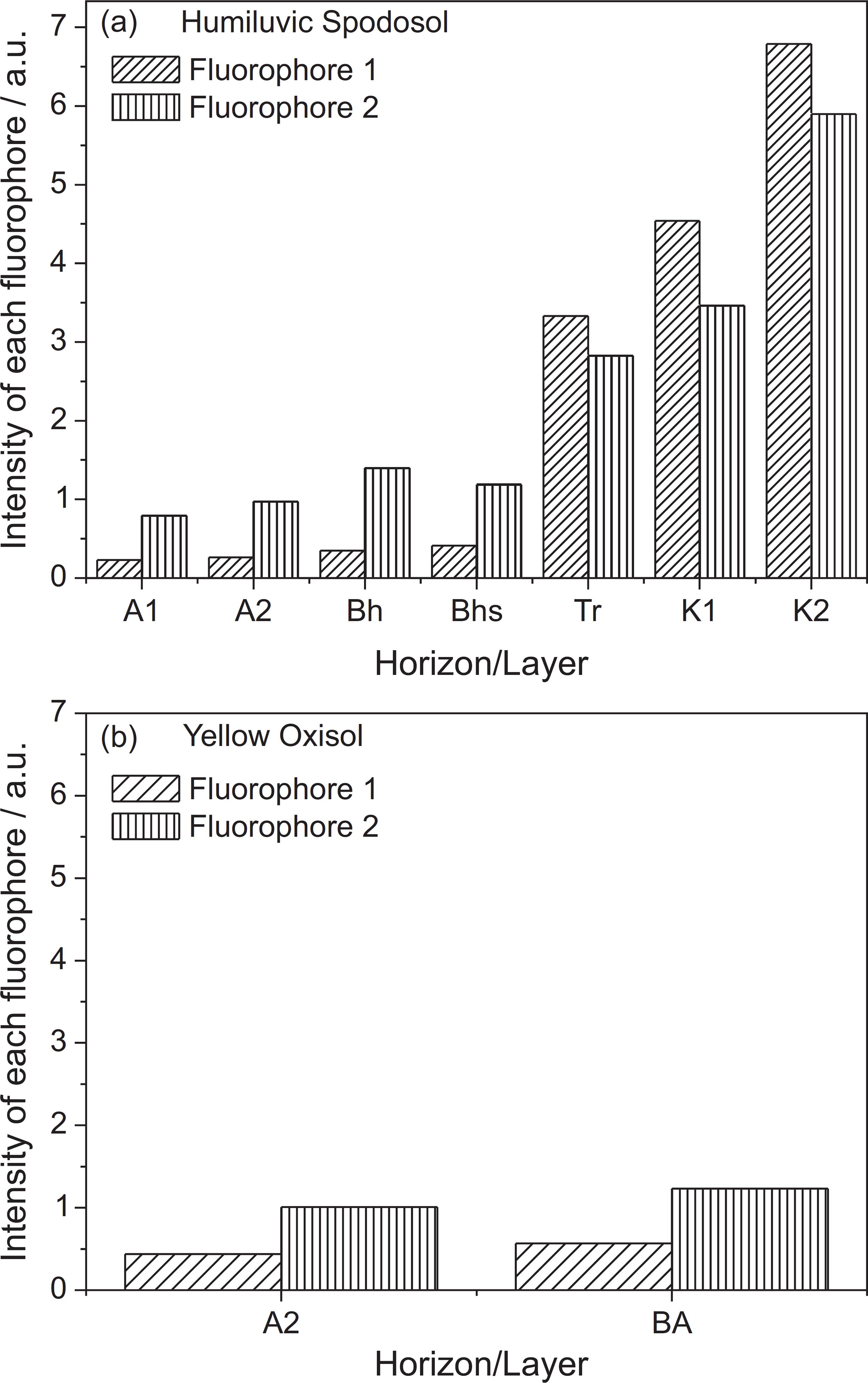
The intensity contribution of each fluorophore in each horizon for Humiluvic Spodosol and Yellow Oxisol is presented in Figures 4a and 4b, respectively.

Figure 4
Contributions to the fluorescence by fluorophores 1 and 2 of the HAs extracted from (a) Humiluvic Spodosol and (b) Yellow Oxisol.

The results show that the chemical structure of HA changed along the profile. For superficial (A1 and A2) and spodic horizon (Bhs), the HA structure has a greater contribution of fluorophore 2, but, at the horizon transition (Tr), this behavior is inverted and the contribution of fluorophore 1 increases and becomes greater than fluorophore 2, both at this horizon and in the deeper horizons of kaolin (K1 and K2) (Figure 4a). On the other hand, for Yellow Oxisol (Figure 4b), there was a more significant contribution of the two fluorophores to surface horizon BA compared to surface horizon A2, highlighting the contribution of fluorophore 2 associated with HAs (groups simpler fluorophores), and this may be attributed to the contribution of OM (gunny) and its own degradation. However, we cannot infer an increasing or decreasing trend in the contribution of fluorophores in depth, because it was not possible to extract HAs for intermediate and deep profiles.

Various models proposed in previously published reports try to explain the structure of HSs, and the macromolecular model is highlighted,⁴⁰ in which the molecular components of HSs are produced by secondary synthesis reactions of degradation products, and the fragments formed by macromolecular aggregates are connected through strong covalent bonds. A new vision has resulted in the development of a HS model, which is composed of supramolecular aggregates of degradation products that come together by entropic interactions and non-covalent bonds.^41-43

This new concept, known as the supramolecular model, exposes that HSs are formed by small and heterogeneous molecules of various origins that self-assemble into supramolecular conformations, which would explain the apparent large molecular size of HSs.^41,44

Thus, the results obtained for Humiluvic Spodosol (Figure 4a) concording with the model of supramolecular structure,^41,44-46 as the ratio of the contribution of fluorophores 1 and 2 does not remain in profile, indicating that there were two types of more recalcitrant HAs (complex structure) and other more labile HAs (simple structure). Moreover, the results do not corroborate the model of macromolecular structure, as the ratio of the contribution of fluorophores 1 and 2 would continue along the profile.

If we consider the macromolecular model for HA, the ratio between the different fluorophores of a molecule should be kept constant along the soil profile. However, in our results, this was not observed. Indeed, a sharp reversal occurs after the transition layer. Thus, it seems that structures identified as fluorophore 1 more readily cross all the soil profile and tend to accumulate on the transition horizon and in the kaolin pores.

These results also corroborate the results of the A₄₆₅ humification index obtained by two-dimensional fluorescence (Figure 1c). The correlations between the humification index and fluorophores obtained by combining EEMs with CP/PARAFAC were very strong (R = 0.95 for the fluorophore 1 and R = 0.88 for the fluorophore2). The combination of EEM in the CP/PARAFAC gives more detailed information, allowed us to identify the contribution of two fluorophores in the structure of the extracted HAs, whereas using methodologies with two-dimensional fluorescence and it is not possible to separate the contribution of the fluorescence for each fluorophore.

Conclusions

EEM fluorescence spectroscopy was more selective and sensitive compared to two-dimensional fluorescence techniques for characterize extracted HAs, showing interesting information about structural variations and the differences between the chromophores that emit fluorescence along depth profile of Humiluvic Spodosol. The combination of EEM and CP/PARAFAC allowed us to quantitatively characterize the HAs, identifying the contribution of the two fluorophores associated with HAs, one linked to complex and another linked to more simple fluorophores with CORCONDIA of 84.2%. For Humiluvic Spodosol, the proportion of the contribution of fluorophores1 and 2 is not maintained along the profile, corroborating the model of supramolecular structure for the HAs.

The combination of EEM fluorescence spectroscopy with CP/PARAFAC may provide information about the processes of transformation of HSs in the soil. It is an interesting analytical method for the study of HSs in such soils, allowing us to quantify the contribution and participation of each fluorophore in fluorescence, compared to two-dimensional fluorescence, which not perform this type of separation.

Acknowledgments

The authors thank FAPESP (Process 2013/13013-3), CNPq, CAPES (Brazilian research funding agencies) and EMBRAPA for financial support of this study.

References

• ¹
  Malhi, Y.; Wood, D.; Baker, T. R.; Wright, J.; Phillips, O. L.; Cochrane, T.; Meir, P.; Chava, J.; Almeida, S.; Arroyo, L.; Higuchi, N.; Killeen, T.; Laurance, S. G.; Laurance, W. F.; Lewis, S. L.; Monteagudo, A.; Neill, D. A.; Vargas, P. N.; Pitman, N. C. A.; Quesada, C. A.; Salomão, R.; Silva, J. N. M.; Lezama, A. T.; Terborgh, J.; Martínez, R. V.; Vinceti, B.; GCB Bioenergy 2006, 12, 1107.
• ²
  Intergovernmental Panel on Climate Change; IPCC: Summary for Policymakers. In: Climate Change 2007: The Physical Science Basis. Contribution of Working Group I to the Fourth Assessment Report of the Intergovernmental Panel on Climate Change; Solomon, S.; Qin, D.; Manning, M.; Chen, Z.; Marquis, M.; Averyt, K. B.; Tignor, M.; Miller, H. L., eds.; Cambridge University Press: Cambridge, United Kingdom and New York, NY, USA, 2007.
• ³
  Lucas, Y.; Chauvel, A.; Boulet, R.; Ranzani, G.; Scatolini, F.; Rev. Bras. Cienc. Solo 1984, 8, 325.
• ⁴
  Lucas, Y.; Montes, C. R.; Mounier, S.; Cazalet, M. L.; Ishida, D.; Achard, R.; Garnier, C.; Melfi, A. J.; Biogeosciences 2012, 9, 3705.
• ⁵
  Schnitzer, M. In Methods of Soil Analysis: Chemical and Microbiological Properties; ASA-SSSA: Madison, 1982.
• ⁶
  Stevenson, F. J.; Humus Chemistry: Genesis, Composition and Reaction, ^2nd ed.; New York: John Wiley & Sons, 1994.
• ⁷
  Dieckow, J.; Mielniczuk, J.; Knicker, H.; Bayer, C.; Dick, D. P.; Kögelknabner, I.; Soil Tillage Res. 2005, 81, 87.
• ⁸
  Zech, W.; Senesi, N.; Guggnberger, G.; Kaiser, K.; Lehmann, J.; Miano, T. M.; Miltner, A.; Schroth, G.; Geoderma 1997, 79, 117.
• ⁹
  Senesi, N.; Anal. Chim. Acta 1990, 232, 51.
• ¹⁰
  Senesi, N.; Miano, T. M.; Provezano, M. R.; Brunetti, G.; Soil Sci 1991, 152, 259.
• ¹¹
  Martin-Neto, L.; Nascimento, O. R.; Talamoni, J.; Poppi, N. R.; Soil Sci 1991, 151, 369.
• ¹²
  Martin-Neto, L.; Rossel, R.; Sposito, G.; Geoderma 1998, 81, 305.
• ¹³
  Martin-Neto, L.; Traghetta, D. G.; Vaz, C. M. P.; Crestana, S.; Sposito, G.; J. Environ. Qual 2001, 30, 520.
• ¹⁴
  Kalbitz, K.; Geyer, W.; Geyer, S.; Biogeochemistry 1999, 47, 219.
• ¹⁵
  Zsolnay, A.; Baigar, E.; Jimenez, M.; Steinweg, B.; Saccomandi, F.; Chemosphere 1999, 38, 45.
• ¹⁶
  Olk, D. C.; Brunetti, G.; Senesi, N.; Soil Sci. Soc. Am. J 2000, 64, 1337.
• ¹⁷
  Bayer, C.; Martin-Neto, L.; Mielniczuk, J.; Saab, S. C.; Milori, D. M. P.; Bagnato, V. S.; Geoderma 2002, 105, 81.
• ¹⁸
  Milori, D. M. B. P.; Martin-Neto, L.; Bayer, C.; Mielniczuk, J.; Bagnato, V. S.; Soil Sci 2002, 167, 739.
• ¹⁹
  Novotny, E. H.; Martin-Neto, L.; Geoderma 2002, 106, 305.
• ²⁰
  Carvalho, E. R.; Martin-Neto, L.; Milori, D. M. B. P.; Rocha, J. C.; Rosa, A. H.; J. Braz. Chem. Soc 2004, 15, 421.
• ²¹
  González-Pérez, M.; Martin-Neto, L.; Saab, S. C.; Novotny, E. H.; Milori, D. M. B. P.; Bagnato, V. S.; Colnago, L. A.; Melo, W. J.; Knicker, H.; Geoderma 2004, 118, 181.
• ²²
  Jouraiphy, A.; Amir, S.; Gharous, M. E.; Revel, J. C.; Hafidi, M.; Int. Biodeterior. Biodegrad. 2005, 56, 101.
• ²³
  Adani, F.; Genevini, P.; Tambone, F.; Montaneri, E.; Chemosphere 2006, 65, 1414.
• ²⁴
  Coble, P. G.; Mar. Chem. 1996, 51, 325.
• ²⁵
  Mc Knight, D. M.; Boyle, E. W.; Westwehoff, P. K.; Doran, P. T.; Kulbe, T.; Anderson, D. T.; Limnol. Oceanogr. 2001, 46, 38.
• ²⁶
  Wu, F. C.; Midorikawa, T.; Tanoue, E.; Geochem. J. 2001, 35, 333.
• ²⁷
  Chen, J.; Gu, B.; Leboeuf, E. J.; Pan, H.; Dai, S.; Chemosphere 2002, 48, 59.
• ²⁸
  Chen, W.; Westerhoff, P.; Leenherr, J.; Booksh, K.; Environ. Sci. Technol. 2003, 37, 5701.
• ²⁹
  Sierra, M. M. D.; Giovanela, M.; Parlanti, E.; Soriano-Sierra, E. J.; J. Braz. Chem. Soc. 2006, 17, 113.
• ³⁰
  Liu, L.; Song, C.; Yan, Z.; Li, F.; Chemosphere 2009, 77, 15.
• ³¹
  Andersen, C. M.; Bro, R.; J. Chemom. 2003, 17, 200.
• ³²
  Stedmon, C. A.; Markager, S.; Estuarine, Coastal Shelf Sci. 2003, 57, 1.
• ³³
  He, X. S.; Xi, B. D.; Li, X.; Pan, H. W.; An, D.; Bai, S. C.; Li, D.; Cui, D. Y.; Chemosphere 2013, 93, 2208.
• ³⁴
  Montes, C. R.; Lucas, Y.; Melfi, A. J.; Ishida, D. A.; C. R. Geosci. 2007, 339, 50.
• ³⁵
  Ishida, D. A.; Montes, C. R.; Lucas, Y.; Pereira, O. J. R.; Merdy, P.; Melfi, A. J.; Eur. J. Soil Sci. 2014, 65, 706.
• ³⁶
  Swift, R. S.; Organic Matter Characterization; Sparks, D.; ed.; Soil Science Society of America: Madison, 1996.
• ³⁷
  Luciani, X.; Mounier, S.; Redon, R.; Bois, A.; Chemom. Intell. Lab. Syst. 2009, 96, 227.
• ³⁸
  Luciani, X.; Mounier, S.; Paraquetti, H. H. M.; Redon, R.; Lucas, Y.; Bois, A.; Lacerda, L. D.; Raynaud, A.; Ripert, A.; Mar. Environ. Res. 2008, 2, 148.
• ³⁹
  Matthews, B. J. H.; Jones, A. C.; Theodorou, N. K.; Tudhope, A. W.; Mar. Chem. 1996, 55, 317.
• ⁴⁰
  Schulten, H. R.; Schnitzer, M.; Soil Sci. 1997, 162, 115.
• ⁴¹
  Piccolo, A.; Soil Sci. 2001, 166, 810.
• ⁴²
  Piccolo, A.; Conte, P.; Trivellone, E.; Van Lagen, B.; Environ. Sci. Technol. 2002, 36, 76.
• ⁴³
  Kleber, M.; Johnson, M. G.; Adv. Agron. 2010, 106, 77.
• ⁴⁴
  Conte, P.; Piccolo, A.; Environ. Sci. Technol. 1999, 33, 1682.
• ⁴⁵
  Simpson, A. J.; Magn. Reson. Chem. 2002, 40, S72.
• ⁴⁶
  Sutton, R.; Sposito, G.; Environ. Sci. Technol. 2005, 39, 9009.

Publication Dates

• Publication in this collection
  June 2015

History

• Received
  15 Jan 2015
• Accepted
  27 Mar 2015