SPC of multiple stream processes: a chart for enhanced detection of shifts in one stream

CEP de Processos com Múltiplos Canais: um gráfico de controle para detecção mais eficiente de alterações em um canal

SPC of multiple stream processes - a chart for enhanced detection of shifts in one stream

CEP de Processos com Múltiplos Canais – um gráfico de controle para detecção mais eficiente de alterações em um canal

Eugenio Kahn Epprecht^I,*; Laura França Marques Barbosa^II; Bruno Francisco Teixeira Simões^III

^[e-mail], PUC-Rio, Brasil

^[e-mail], PUC-Rio, Brasil

^[e-mail], PUC-Rio, Brasil

ABSTRACT

The efficiency of Boyd's group charts -the classical scheme for the statistical control of multiple-stream processes- is impaired by its underlying model of the process not considering that part of the variation in such processes is common to all streams. Mortell and Runger (1995) and Runger, Alt and Montgomery (1996) proposed alternative schemes which take this fact into account. We propose a third scheme: a modified group chart, based on the differences between the values of the quality characteristic in each particular stream and the average of the values of all streams. The average run lengths of this scheme and of the competing schemes in the case of shifts in the mean of one individual stream are obtained either analytically or by simulation and compared. The results show the superiority of the proposed scheme except for shifts smaller than one standard deviation, against which no one of the schemes is really efficient.

Keywords: Multiple stream processes. Group charts. Statistical process control. Performance analysis. ARL.

RESUMO

A eficiência dos gráficos de controle de grupos propostos por Boyd -o esquema clássico para controle de processos com múltiplos canais (ou multifluxo)- é comprometida porque o modelo de processo em que se baseiam não leva em conta que uma parte da variabilidade neste tipo de processos é comum a todos os canais. Mortell & Runger e Runger et al. propuseram esquemas de controle alternativos que levam esse fato em conta. Neste trabalho é proposto um terceiro esquema: um gráfico de controle de grupos modificado, baseado nas diferenças entre os valores da característica de qualidade em cada canal e a média dos seus valores em todos os canais. Os números médios de amostras até o sinal (ou comprimentos médios de corrida) desse esquema e dos esquemas concorrentes são obtidos analiticamente ou por simulação, para o caso de alterações na média de um canal individual, e comparados. Os resultados mostram a superioridade do esquema proposto exceto para o caso de alterações na média de magnitude inferior a um desvio-padrão, caso porém em que nenhum dos esquemas é eficiente.

Palavras-chave: Processos com múltiplos canais. Processos multifluxo. Gráficos de controle de grupos. Controle Estatístico de Processos. Análise de desempenho. NMA.

1. Introduction

A multiple stream process (MSP) is a process that generates several streams of output. From the statistical process control standpoint, the quality variable and its specifications are the same in all streams. A classical example is a filling process such as the ones found in beverage, cosmetics, pharmaceutical and chemical industries, where a filler machine may have many heads. Another example would be a mould with several cavities. Other processes may still produce only one stream of output but the quality variable may be measured at several points at a same time. Consider for instance the fabrication of paper, sheets of steel, or the production of rubber hoses by extrusion, where at every sampling time, the thickness of the outcoming material is measured in different locations of its section. For the purposes of modelling and monitoring, these can also be seen as multiple stream processes.

Although multiple-stream processes are very frequent in industry, the literature on SPC schemes for such kind of processes is far from abundant. The earliest work is Boyd (1950), which proposes the group control chart (GCC). Nelson (1986) developed a runs rule to enhance the detection ability of the GCC, and Ott and Snee (1973) present an exhaustive off-line analysis of an MSP, discussing different subgrouping and charting strategies. Until the mid-90's, a pair of GCCs (one for averages and other for ranges) used together with Nelson's runs rule remained as virtually the only specific procedure for monitoring MSPs. It is the scheme recommended in main texts on SPC, such as Montgomery's classic book, up to the 3^rd ed. (MONTGOMERY, 1997, Section 8.3) (in later editions, there is reference to the new theory) or Pyzdek (1992, Chapter 21).

The classic GCCs are based (at least implicitly, in the way their statistics and control limits are calculated) on the assumption that the streams are independent from each other. This assumption is not realistic in practice about most MSPs, due to the presence of a component of the quality variable which is common to all streams, resulting in significant cross-correlations between them. Mortell and Runger (1995) were the first to acknowledge this process structure, representing the value of the quality variable measured in any stream as the sum of two components: a part common to all streams plus the individual (residual) component of each stream.

They propose therefore controlling the process with a pair of charts: anchart for the average of all streams -sensitive to changes in the common component- and an R chart for the statistic R_t - the range between streams (or between stream averages, in the case of more than one observation per stream) - sensitive to changes in the individual components. They convincingly illustrate why this scheme is more efficient than the GCC in signalling special causes that affect individual streams.

Runger, Alt and Montgomery (1996), based on the same process model, analyze an alternative scheme, which employs an S² chart on the variance between streams in the place of the R_t chart (Modelling the MSP as a multivariate process and considering its decomposition in principal components, they show that the first PC is the average between all streams and the S² statistic is equivalent to the Hotelling's T² statistic of all other PCs). Also, one can view both the R_t and the S² statistics simply as two alternative measures of dispersion between streams and thereby sensitive to departures of one or some of the streams from the group.

Other recent works are: Lanning, Montgomery and Runger (2002), who evaluate a variable-sampling interval scheme for MSP, and Liu, Mackay and Steiner (2008), who model the problem of controlling the output of a production process with several gauges in parallel. However, these works do not apply to the situations we are concerned with in this paper. Lanning, Montgomery and Runger (2002) consider processes where most of the assignable causes affect all streams, and shifts in a single stream are rare and of little practical relevance. In other words, they tackle the problem of detecting shifts in the common component. From the mathematical perspective, the MSP they consider is similar to a classic univariate process. Indeed, they view the measures of the quality variable in the different streams as a homogeneous random sample from a same population. The control scheme they propose is exactly the VSI Shewhart chart proposed and analyzed by Reynolds (1989). In the situation considered by Liu, Mackay and Steiner (2008), the production units are independent and, even if they consider that there are special causes that affect one particular stream (gauge) and special causes that affect all streams (causes acting on the production process), there is no such thing as a "common component" that introduces cross-correlation between streams in a same sampling time (moreover, the measurements in different streams -gauges- are never simultaneous).

Meneces et al. (2008) use simulation to compare the in-control performance of three schemes for the statistical control of MSPs: the group method, the R_t chart proposed by Mortell and Runger (1995) and a separate Shewhart chart for each stream. For the group method they consider only Nelson's (1986) runs criterion, without any control limit as in Boyd (1950). In conclusion, they recommend using one chart for each stream, for two reasons: because of its diagnostic feature (for example, when the R_t chart signals, an investigation is needed to determine which stream(s) is (are) affected by special causes), and because this scheme is more robust to differences in centering between different streams (it admits adjusting for this case, through simply replacing the observation in one stream by its difference to the in-control mean of the stream; the other methods would exhibit too many false alarms in this case). Next, they analyze the out-of-control performance of the one-chart-for-each-stream method. They also provide values for the control limits coefficients of the Shewhart charts that yield the desired in-control ARL, as a function of the correlation between streams. Although they acknowledge the presence of such correlation, they do not consider separating the two components of variability (common variability and intra-stream variability), as the individual charts they recommend use directly, as monitoring statistics, the values observed in each stream - the same monitoring statistics used by Boyd's group charts with control limits. This may lead to the same drawback of these charts, namely, reduced sensitivity to special causes that affect just one or a few streams, as we are going to discuss in the next section of this paper.

Mortell and Runger (1995) mention still the possibility (which they do not explore) of controlling the individual components of the streams by the residuals of each stream, that is, the differences between each stream observation (or each stream average) and the average (or grand average) of all streams.

This paper proposes a group chart for such residuals, and analyzes its performance against shifts in the mean or in the variance of one individual stream. The analysis shows that the efficiency of the residuals group chart against shifts in the mean of one stream is in most cases superior to the efficiency of the other existing schemes (MORTELL; RUNGER, 1995; RUNGER; ALT; MONTGOMERY, 1996).

The residuals GCC is not more complex or cumbersome to implement than the R_t or the S² chart if a spreadsheet is available, and, in contrast with these procedures, it clearly indicates which streams are likely to be out-of-control.

The remainder of this paper is organized as follows: the next section details the model of multiple stream processes considered in this paper, as well as the previous control schemes that are competitors of the one here proposed. This constitutes the necessary background for the understanding of the description of the proposed control scheme, in Section 3. Next, Section 4 details some peculiarities of this scheme and introduces the model for obtaining its performance measures. Using these measures, the performance of the scheme is compared with the performance of its competitors, in Section 5. Section 6 summarizes the conclusions of the analysis.

2. Background: group control charts, process model and related works

The motivation for the group control charts (GCC) proposed by Boyd (1950) and described in Burr (1976), Pyzdek (1992, Chapter 21) and Montgomery (1997, Section 8.3), is to avoid the proliferation of control charts that would arise if every stream were controlled with a separate pair of charts. Assuming that the in-control distribution of the quality variable is the same in all streams, the control limits should be the same for every stream. So, the basic idea is to build only one chart (or a pair of charts) with the information from all streams. Specifically: at each sampling time t, every stream i is sampled and the corresponding _i and R_i are calculated; the largest and the smallest are plotted in the group control chart, and the largest R is plotted in the R group control chart. If these points are within the control limits, the other points (not plotted) would necessarily be within the limits, too. Figure 1 illustrates the procedure.

The GCC will work well if the values of the quality variable in the different streams are independent and identically distributed, that is, if there is no cross-correlation between streams. However, such an assumption is often unrealistic. In many real multiple stream processes, the value of the observed quality variable is typically better described as the sum of two components: a common component (let's refer to it as "base level"), exhibiting variation that affects all streams in the same way, and the individual component of each stream, which corresponds to the difference between the stream observation and the common base level. The base level values over time may be i.i.d. or exhibit some dynamical behavior. In formal notation: supposing that at time t a subgroup of n measures is taken at each stream of an m-stream process, the value of the j-th observation of the quality variable in stream i in time t is given by:

where b_t is the value of the "base level" in time t, and e_tij is the value of the the j-th observation of the individual component of in the i-th stream at time t. Additionally, e_tijis assumed to be i.i.d. ~N(0,σ²) over t, i and j, and independent from b.

As a result, the variance of the values of

_i (the sample average of the observations in any stream i) observed along the time is

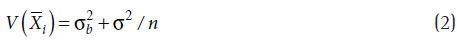
where σ_b² is the variance of the base level over time.

The presence of the base level component can be identified in a given MSP by examining the correlations between different streams (that is, between the

_ti's: the averages over j of the n values observed in each stream i in a same time t), because the base level introduces cross-correlations between the streams. Indeed, the correlation between the averages of any two streams i and p is .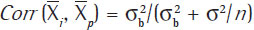

Since the control limits of the GCC should be based on the total variance of _i -and ideally should still be "widened" according to Bonferroni's (JOHNSON; WICHERN, 2007) or Dunn-Sidak (DUNN, 1958; SIDAK, 1967) correction as a function of the number of streams, to avoid inflating the total false‑alarm rate-, the presence of the base level component leads to reduced sensitivity of Boyd's GCC to shifts in the individual component of a stream if σ_b² (the variance of the base level) is large with respect to σ² (the variance of the individual stream components).

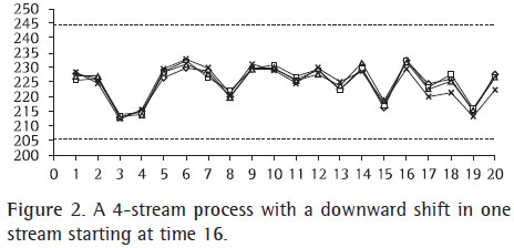
To illustrate this issue, Figure 2 presents the time plots of 4 streams of a process well described by Equation 1 with σ_b = 5σ and one observation per stream. The data were artificially generated, and a sustained downward shift of magnitude 3σ was applied to the mean of one of the streams from time 16 on. It is easy to see that this shift would take a long time to generate a signal.

Nelson (1986) has proposed an additional runs criterion for GCCs, which would be sensitive to shifts in one stream, even in a process of this kind. Each point plotted in the GCC should be marked, identifying the stream that yielded the extreme value. If the same stream appears more than r times in a row (where the threshold value r is a value that is statistically significant and thus depends on the number of streams of the process), then there is evidence that that particular stream has shifted. Wise and Fair (1998) recommend using only Nelson's criterion, without any control limit.

Unfortunately, the runs criterion has two limitations: first, if two or more streams shift, they are likely to alternate the extreme reading, so it may take much time to observe a run of r consecutive observations of just one stream. In addition, due to the discreteness of r, for some numbers of streams in the process, there is no good value for r, in the sense that for any value the false-alarm risk is either too high or too low (the problem with the latter case is that this comes along with reduced sensitivity to shifts); so there is no r value that corresponds to a good tradeoff between false-alarm risk and power. This fact has already been pointed out by Mortell and Runger (1995) and reported by Montgomery (1997, 2001).

To monitor MSPs with the two components described, Mortell and Runger (1995) propose using two control charts: first, a chart for the grand average between streams, to monitor the base level. The type of chart to be used should be chosen according to the dynamics of the base level: if it corresponds to a "Shewhart process" (constant mean, no serial correlation), a classical chart, or an EWMA or CUSUM chart would be appropriate; if it exhibits autocorrelation, some procedure for monitoring an autocorrelated process should be used. In any case, it would be a known procedure in the previous literature for univariate processes, so Mortell and Runger (1995) do not focus on it.

The focus of their paper is the chart for monitoring the individual stream components: they propose using a range chart (R_t chart), whose statistics is the range between streams, that is, the difference between the largest stream average and the smallest stream average (at any time t, the n values x_tij in each stream i are averaged; R_t is then the difference between the maximum and the minimum of these averages). If the process is in control and all individual stream components have mean equal to zero, the R_t statistic has mean d₂σ and standard deviation d₃σ, where the constants d₂ and d₃ are based on a "sample size" of m, the number of streams. If a stream undergoes a shift in the mean, R_t will increase, as it is evident in Figure 2.

Runger, Alt and Montgomery (1996) propose a similar scheme, with a chart for the grand average between streams, to monitor the base level, and an S² chart in the place of the R_t chart. Analogously to the R_t chart, if there is more than one observation per stream, these should be averaged (in the stream) to yield only one value per stream. The sample size for calculating S² is the number of streams.

3. Proposed control scheme: the residuals group control chart

The purpose of this paper is to propose an alternative control scheme for monitoring the individual stream components of MSPs described by Equation 1 and to analyze its performance, comparing it with the performance of Mortell and Runger's R_t chart and Runger et al.'s S² chart in the case of sustained shifts (step changes) in the mean of one individual stream. Like those previous authors, we recommend this scheme to be used together with a chart for the grand average between streams to monitor the base level, but this chart is not in the scope of the paper. The focus is on monitoring for shifts in the mean of any individual stream.

The idea is to monitor the individual components -the e_tij's. These, however, are not directly observable, since each observation x_tij is the sum of the individual component and the unobservable base level. These two components (base level and individual component) can be estimated by:

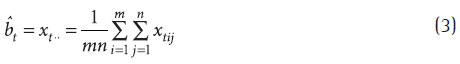
that is, the grand average of all the observations, and

that is, the residual of each observation relative to the estimate of the base level.

The control statistic for each stream is the average over j (that is, the stream subgroup average) of the ê_tij's, given by

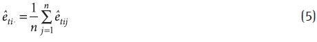
or alternatively by

where the dot replacing an index (in this case, j) indicates averaging over that index (differently from the usual notation where the dot means summation and an additional bar would be required to indicate averaging, we drop the bar for the sake of keeping the notation cleaner).

The scheme proposed is a group control chart on the ê_ti's, which we call the residuals GCC.

The operation of the chart is identical to the operation of Boyd's GCC for the averages: at each sampling time, the statistics are calculated, the maximum and the minimum ê_ti are plotted in the chart and a signal is given if any of them is outside the control limits. The differences to Boyd's classic GCC lie on the statistics used and on the calculation of the control limits. There are, also, a number of peculiarities with this scheme, which should be taken into account when designing the chart, and are described in the next section, together with the expressions of the standard deviations of the residuals for determination of the control limits.

Finally, we may consider that when the maximum or minimum residual is outside the limits, the user should check if any other residual is also outside the limits; this is easy to do considering that the procedure will be implemented in a spreadsheet or other software, which is easy to program to indicate any value outside the limits, by conditional formatting, for example. So, more than one stream may signal at a time.

4. Peculiarities and performance measures of the proposed chart

While the e_tij's are i.i.d. over t, i and j, with variance σ², the residuals from different streams are cross-correlated. Using Equations 3 and 6 in the usual expressions for calculating variances and covariances, it can be easily shown that the correlation between the residuals of any pair of streams i and p, i ≠p, (and also between their averages ê_tiand ê_tp) is

It can also be shown that the standard deviation of ê_tiis

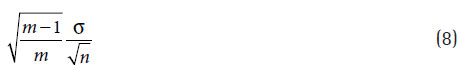
As a result, the control limits are

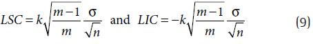
The value of the control limit coefficient k that keeps the overall false-alarm risk (the probability of at least one of the ê_ti's falling out of the control limits with the process in control) at a desired level α_global will depend on the number of streams. If the ê_ti's were independent of each other, the adjustment of k for the number of streams should follow the Dunn-Sidak correction (DUNN, 1958; SIDAK, 1967), namely:

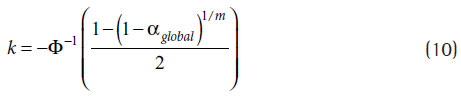
where Ф^-1 (.) is the inverse standard normal distribution function.

This correction would be precise and result in an actual overall false-alarm risk equal to the α_global value specified if the residuals from different streams were not cross-correlated. Because as a matter of fact they are, calculation of the global false-alarm probability requires integrating the multivariate (m-variate) normal distribution over the m-dimensional hypercube corresponding to the in-control region (within the control limits). We have done this, obtaining the following exact values for k, for α_global values of 0.01, 0.05 and 0.0027, which correspond to in-control ARL (ARL₀) values of 100, 200 and 370.4 respectively:

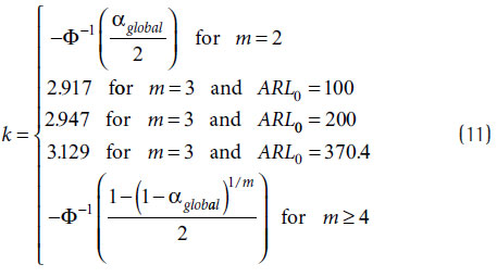
It can be seen that with m = 2 no correction is made; the expression for k is the same as for the control limit coefficient of the traditional (univeriate) chart. Indeed, in a two-stream process, the residuals of the two streams are perfectly correlated, with ρ₁₂ = -1, so they always signal together. With m ≥ 4, on the other hand, k may be calculated by (10), neglecting the cross-correlation effect. Indeed, we have found that for more than three streams the Dunn-Sidak's correction yields good results in practical terms. The actual ARL₀ would be slightly greater than specified, but the difference would be of less than 5% already for m = 4.

Note that the expressions of the control limits in (9) are based on the real standard deviation of the individual components, σ, which is unknown by definition. The factor should only be used if the standard deviation is known. For instance, expressions 9 were used in this work since the performance measures were obtained via simulation, using data generated according to a given σ. When using the control scheme in practice, the standard deviation should be estimated from past data, taking the residuals to the base level and directly estimating its standard deviation according to some estimator or other - see Mahmoud et al. (2010), about the issue of the best estimator). This estimate should then replace in expressions 9.

Another peculiarity of the proposed scheme is that a shift of magnitude δσ in the mean of one of the e_i(t)'s introduces a bias of magnitude -δσ/s in which in its turn introduces a bias in all ê_ti 's, with magnitude -δσ/m. As a consequence, the probability of a signal associated to another stream and also the probability of a signal by the chart for the base level increase a bit. For the stream that shifted, E (ê_ti) = [(m - 1)/m]δs.

So, unlike what happens in the univariate (or single stream) case, there are multiple possible types of signal when the individual component of stream i undergoes a shift: a signal associated to stream i (ê_ti outside the limits), which we may call a "correct" alarm; a signal associated to another stream, p (ê_tp outside the limits, with p ≠ i) or even to more than one stream different than stream i; and also a signal in the chart for the base level. Whether signals associated to the base level or to other streams than the one that actually shifted (which we may call "incorrect" alarms) should be regarded as true or false alarms will depend on the reaction to these signals. If the strategy, when there is a signal, is to investigate only the stream associated to the signal, only signals on the stream that shifted serve as true alarms (whether accompanied or not by other signals); if, however, any signal leads to an investigation of all streams (at least if no anomaly is found in the stream that issued the signal after a first investigation), then any alarm serves as a true alarm.

Figure 3 illustrates the relevant events related to signals.

Although the probabilities of a signal in a given stream can be calculated analytically, the probabilities of the composite events can not, since the events are not independent, so the binomial distribution does not apply. Moreover, for some signal events an ARL may not even be defined (viz. the incorrect alarms O-A and (OB)-A), since the "run" until the incorrect alarm may be interrupted by a correct signal).

For the performance analysis, we cannot disconsider without examination the probability of true but incorrect signals. However, as the numerical results of the analysis have shown, the probabilities of the event O-A (only incorrect alarms) are very small -of the order of the false-alarm probability (P(O-A) <0.005 in general, and always <0.010. The larger values occur when the probability of correct signal -the event A- is larger, which reduces the probability of incorrect signal given that a signal occurred). The probability of the event B (signal in the chart for the base level due to a shift in one stream) will depend on the dynamics of the base level -especially on the ratio between its variance and the variance of the individual stream components- and on the type of chart used to control it, but it can be expected to be smaller than the probability of a signal in a stream not affected by the special cause. This can be expected because of the variance of the base level, which makes the bias mentioned before less influent for this chart than for other streams in the residuals GCC (bear also in mind that there are m-1 non affected streams, increasing the possibilities for the event O, whereas there is only one base level estimate, so if the probabilities of the event O-A are very small, then the probabilities of B-A should be smaller). The practical conclusion is that either the event A or the event A O may be considered for the performance evaluation of the scheme and that, although theoretically incorrect signals may be a drawback of the proposed residuals GCC, in practice they are not an issue. Table 1 details the events and ARLs of interest.

5. Performance comparison with competing control schemes

Table 2 shows the out-of-control ARL's of the residuals GCC and of Mortell and Runger's R_t chart for several magnitudes of shift in the individual component of one stream of the process, several numbers of streams and three overall ARL₀ values, considering one observation per stream at each sampling time (n = 1). The ARL's were obtained considering as "true signal" a signal in any one of the streams (event AO). The shifts (δ) are measured in units of standard deviation of the individual component. The values were obtained via simulation, due to the peculiarities explained in the previous section of the control scheme, which prevent obtaining the probability of the event AO analytically. For each combination (shift, number of streams, ARL₀ specified), 160000 samples were generated to obtain the proportion of signals. This leads to a standard error smaller than 1.8% for ARL = 50, and decaying for smaller ARL values (1.1% for ARL = 20; 0.75% for ARL = 10; 0.5% for ARL = 5; 0.025% for ARL = 2).

Table 3 shows the percent differences between the ARL's of the two schemes. The differences are of the residuals GCC ARL relative to the R_t chart ARL, that is, negative values correspond to a smaller ARL of the residuals GCC chart.

It can be seen from Tables 2, 3 and 4 that:

• The residuals GCC gives smaller ARL's than the R_t chart, except for shifts in the mean of the magnitude of 1 standard deviation or less

• ... but no one of the schemes is efficient for shifts of less than 2 standard deviations (with n = 1) or shifts of less than 1 standard deviation (with n = 5)

• ... which by the way may be irrelevant to detect if σ_b/σ > 1 (because they would correspond to much smaller shifts in units of the total standard deviation of the process).

• The advantage of the residuals GCC increases with the number of streams.

Of course the ARL's are greatly reduced if subgroups are taken instead of individual observations per stream. Table 4 shows the ARLs if n = 5. The relative behavior of the two schemes, however, remains essentialy the same as with n = 1. Only the shift magnitude for which one scheme becomes more efficient than the other is reduced. The R_t chart gives smaller ARL's only for shifts of 0.5 standard deviations (and not for any number of streams nor for any value of ARL₀), but for this magnitude of shift neither of the two schemes is really efficient.

Tables for n = 2, 3 and 4 are omitted for reasons of space and are available from the authors.

Now let's consider Runger et al.'s S² chart. Table 5 compares its ARLs with the ARLs of the R_t chart, for some magnitudes of shift in one stream of the process. It shows that for shifts in one stream, the R_t chart is at least as fast as the S² chart (Indeed, Runger, Alt and Montgomery (1996), have shown that the S² chart performs better when a large number of streams shift, which is not the situation we are concerned about. The performance of the residuals GCC and of the R_t chart in this case is a question for future research. Maybe the base level chart would be enough responsive in this case, though one cannot tell without further investigation. If, however, special causes affect one stream at a time, disturbances are likely to occur first in only one stream, and it is important to have a control scheme that is sensitive to such disturbances).

The important conclusion is that, since the R_t chart is at least as fast as the S² chart, and the residuals GCC proposed is faster than the R_t chart (for most of the shifts that are likely to be relevant to detect quickly), then the proposed scheme becomes the most efficient for detecting shifts in one stream.

6. Conclusions

Although multiple stream processes are common in industry, there are few techniques for the statistical control of such processes. Until 15 years ago, the literature had not yet acknowledged that quality characteristics of many typical multiple stream processes may be thought of as decomposable in two parts, a part common to all streams and the individual component of each stream. Previously to this paper, only two works in the literature proposed control schemes based on such model. We propose a third scheme, and show that it is faster than those previous schemes at detecting shifts in the mean of one stream. The gain in performance with this scheme relative to the other ones increases with the number of streams.

The proposed scheme is outperformed by other schemes only in the case of shifts smaller than one standard deviation of the individual stream component. It should be noted, however, that none of the schemes is efficient at detecting such shifts, and that such shifts may not be relevant in the context of multiple stream processes, where the variance of the individual stream component is just a part of the total process variance.

The proposed residuals group control chart is not more complex to implement than its competitors, Mortell and Runger's R_t chart and Runger et al.'s S² chart, which employ just one statistic, since all the three schemes require taking measurements of the quality variable in every stream, and just compute different sample statistics with these data. If the data are input in software, none of the three schemes is simpler or more complex than the other ones. Taking the residuals enables identifying which ones are beyond the limits, indicating the affected streams, which is an additional advantage of the proposed scheme. The other two schemes of course enable identifying the stream with maximum and with minimum values, but they do not directly identify which ones have significantly large values, since they establish no thresholds for the values themselves.

If theoretically the residuals GCC would apparently have some drawbacks in terms of correlated statistics (since the separation it provides between the two components is not perfect), consequent biases on the statistics of other streams when one of the streams shifts, and probabilities of "incorrect" signals (signals in other streams than the one that has shifted), the numerical analysis of these probabilities have shown that in practice they are too small to become a disadvantage. The probabilities of such signals are of the magnitude of the false-alarm probability. So, in summary, better detection performance and better diagnostic ability make the proposed scheme the most advantageous of all.

The purpose of this paper was to propose a GCC using the residuals as a new monitoring statistics, present its peculiarities, and compare its performance with the existing competing schemes for monitoring multiple stream processes. It was restricted to the Shewhart version of the proposed chart. Mortell and Runger (1995) and Runger, Alt and Montgomery (1996) have also evaluated enhancements to their schemes, in particular EWMA versions of them. The EWMA version of the residuals GCC (and its performance comparison with these competitors) is a natural follow-up of this research and will be the topic of a forthcoming paper.

Acknowledgements

The first and third authors acknowledge the support of the CNPq (Conselho Nacional do Desenvolvimento Científico e Tecnológico, Brazil) and the second author acknowledges the support of the CAPES (Coordenação de Aperfeiçoamento de Pessoal de Nível Superior), Brazil.

References

BOYD, D. F. Applying the group chart for Xbar and R. Industrial Quality Control, v. 7, p. 22-25, 1950.

BURR, I. W. Statistical Quality Control Methods. Marcel Dekker, 1976.

DUNN, O. J. Estimation of the means of dependent variables. Annals of Mathematical Statistics, v. 29, p. 2775-2790, 1958. doi:10.1214/aoms/1177706443

JOHNSON, R. A.; WICHERN, D. W. Applied multivariate statistical analysis. 6. ed. Pearson Prentice Hall, 2007.

LANNING, J. W.; MONTGOMERY, D. C.; RUNGER, G. C. Monitoring a multiple stream filling operation using fractional samples. Quality Engineering, v. 15, n. 2, p. 183-195, 2002. doi:10.1081/QEN-120015851

LIU, X.; MACKAY, R. J.; STEINER, S. H. Monitoring multiple stream processes. Quality Engineering, v. 20, p. 296-308, 2008. doi:10.1080/08982110802035404

MAHMOUD, M. A. et al. Estimating the standard deviation in quality control applications. Journal of Quality Technology (in press), 2010.

MENECES, N. S. et al. Statistical control of multiple-stream processes: a shewhart control chart for each stream. Quality Engineering, v. 20, p. 185-194, 2008. doi:10.1080/08982110701241608

MONTGOMERY, D. C. Introduction to Statistical Quality Control. 3 ed. John Wiley, 1997.

MONTGOMERY, D. C. Introduction to Statistical Quality Control. 4 ed. John Wiley, 2001.

MORTELL, R. R.; RUNGER, G. C. Statistical process control for multiple stream processes. Journal of Quality Technology, v. 27, n. 1, p. 1-12, 1995.

NELSON, L. S. Control chart for multiple stream processes. Journal of Quality Technology, v. 18, n. 4, p. 225-226, 1986.

OTT, E. R.; SNEE, R. D. Identifying useful differences in a multiple-head machine. Journal of Quality Technology, v. 5, n. 2, p. 47-57, 1973.

PYZDEK, T. Pyzdek's Guide to SPC: applications and special topics. ASQ Quality Press, 1992. v. 2.

REYNOLDS JUNIOR, M. R. Optimal variable sampling interval control charts. Sequential Analysis, v. 8, p. 361-379, 1989. doi:10.1080/07474948908836187

RUNGER, G. C.; ALT, F. B.; MONTGOMERY, D. C. Controlling multiple stream processes with principal components. International Journal of Production Research, v. 34, n. 11, p. 2991-2999, 1996. doi:10.1080/00207549608905074

SIDAK, Z. Rectangular confidence regions for the means of multivariate normal distribution. Journal of the American Statistical Association, v. 62, p. 626-633, 1967. doi:10.2307/2283989

WISE, S. A.; FAIR, D. C. Innovative control charting - practical spc solutions for today's manufacturing environment. ASQ Quality Press, 1998.

Recebido 02/09/2010; Aceito 08/02/2011

*

PUC-Rio, Rio de Janeiro, RJ, Brasil

Publication Dates

• Publication in this collection
  29 Apr 2011
• Date of issue
  June 2011

History

• Received
  02 Sept 2010
• Accepted
  08 Feb 2011