Spatio-temporal modelling of coffee berry borer infestation patterns accounting for inflation of zeroes and missing values

Modelagem espaço-temporal do padrão de infestação da broca do café levando em consideração excesso de zeros e dados faltantes

STATISTICS

Spatio-temporal modelling of coffee berry borer infestation patterns accounting for inflation of zeroes and missing values

Modelagem espaço-temporal do padrão de infestação da broca do café levando em consideração excesso de zeros e dados faltantes

Ramiro Ruiz-Cárdenas^{I, II}; Renato Martins Assunção^II; Clarice Garcia Borges Demétrio^{I, *}

^IUSP/ESALQ - Depto. de Ciências Exatas, C.P. 09 - 13418-900 - Piracicaba, SP - Brasil

^IIUFMG - Depto. de Estatística - 31270-901 - Belo Horizonte, MG - Brasil

ABSTRACT

The study of pest distributions in space and time in agricultural systems provides important information for the optimization of integrated pest management programs and for the planning of experiments. Two statistical problems commonly associated to the space-time modelling of data that hinder its implementation are the excess of zero counts and the presence of missing values due to the adopted sampling scheme. These problems are considered in the present article. Data of coffee berry borer infestation collected under Colombian field conditions are used to study the spatio-temporal evolution of the pest infestation. The dispersion of the pest starting from initial focuses of infestation was modelled considering linear and quadratic infestation growth trends as well as different combinations of random effects representing both spatially and not spatially structured variability. The analysis was accomplished under a hierarchical Bayesian approach. The missing values were dealt with by means of multiple imputation. Additionally, a mixture model was proposed to take into account the excess of zeroes in the beginning of the infestation. In general, quadratic models had a better fit than linear models. The use of spatially structured parameters also allowed a clearer identification of the temporal increase or decrease of infestation patterns. However, neither of the space-time models based on standard distributions was able to properly describe the excess of zero counts in the beginning of the infestation. This overdispersed pattern was correctly modelled by the mixture space-time models, which had a better performance than their counterpart without a mixture component.

Key words: Markov chain Monte Carlo methods, risk maps, mixture model, zero inflated model, multiple imputation

RESUMO

O estudo da distribuição de pragas em espaço e tempo em sistemas agrícolas fornece informação importante para a otimização de programas de manejo integrado de pragas e para o planejamento de experimentos. Dois problemas estatísticos comumente associados à modelagem espaço-temporal desse tipo de dados que dificultam sua implementação são o excesso de zeros nas contagens e a presença de dados faltantes devido ao esquema de amostragem adotado. Esses problemas são considerados no presente artigo. Para estudar a evolução da infestação da broca do café a partir de focos iniciais de infestação foram usados dados de infestação da praga coletados em condições de campo na Colômbia. Foram considerados modelos com tendência de crescimento da infestação linear e quadrática, assim como diferentes combinações de efeitos aleatórios representando variabilidade espacialmente estruturada e não estruturada. As análises foram feitas sob uma abordagem Bayesiana hierárquica. O método de imputação múltipla foi usado para abordar o problema de dados faltantes. Adicionalmente, foi proposto um modelo de mistura para levar em consideração o excesso de zeros nas contagens no início da infestação. Em geral, os modelos quadráticos tiveram um melhor ajuste que os modelos lineares. O uso de parâmetros espacialmente estruturados permitiu uma identificação mais clara dos padrões temporais de acréscimo ou decréscimo na infestação. No entanto, nenhum dos modelos espaço-tempo baseados em distribuições padrões descreveu, apropriadamente, o excesso de zeros no início da infestação. Esse padrão de sobredispersão foi corretamente modelado pelos modelos de mistura espaço-tempo, os quais tiveram um melhor desempenho que seus homólogos sem mistura.

Palavras-chave: Métodos Monte Carlo via cadeias de Markov, mapas de risco, modelo de mistura, modelo inflacionado de zeros, imputação múltipla

INTRODUCTION

The coffee berry borer, Hypothenemus hampei Ferrari (Coleoptera: Scolytidae), has been considered as the most important pest of the coffee growing in the world (Jaramillo et al., 2006). That insect attacks directly the fruit of coffee in development making its entire biological cycle inside of them. It uses the fruit as a refuge to reproduce and to feed its offspring, and as shelter from predators and from adverse weather (Le Pelley, 1968) causing severe losses in the grains production and quality. This pest was registered for the first time in Colombia in 1988 and it is present nowadays in more than 700 thousand hectares (85% of the planted area). It has been estimated that the costs of the borer control in Colombia are around of U$100 million a year representing about 10% of the total cost of the coffee production (source: http://pest.cabweb.org/Archive/ Pestofmonth/pest9710.htm. Accessed 10 Jan. 2008).

A detailed description of the coffee berry borer space-time dispersion in commercial fields is important for the better use of control agents in integrated pest management programs, for the development of sampling plans and for the planning of field experiments, among other applications. Some aspects of the dispersion pattern and of sampling strategies for this pest were studied in several countries, showing that the pest has an aggregated distribution pattern in the field (e.g. Ruiz et al., 2000 and references therein).

Although these reports suggested the presence of a spatial pattern in the dispersion of the pest, they did not take into account either the samples spatial location or the spatial scale effect. In fact, the spatio-temporal pattern of insect populations in commercial fields has rarely been studied due to the required intensive sampling effort to obtain spatial information and the limitations of the available statistical methodology until few years ago.

In this study the spatio-temporal variation of the coffee berry borer infestation is analysed under field conditions in Colombia. Statistical models that describe properly the dispersion of the pest in a coffee plot are used, starting from initial focuses of infestation. These methods take into account two difficulties that are common in the practice of spatial data analysis. One is the presence of an excessive number of zero counts with respect to what can be modelled by the usual discrete probability distributions. The other difficulty is the presence of missing values which makes the space-time dispersion modelling more complicated. Based on the results maps are made to identify infestation trends through time.

MATERIAL AND METHODS

Spatio-temporal Statistical Models

There are many deterministic models for insect's spatial and temporal ecological distribution processes, frequently focused on issues of epidemics on large spatial scales (e.g. Rudd & Gandour, 1985; Brewster & Allen, 1997). However, this type of models is not appropriate for studies in small geographical scales, as those frequently observed in experimental systems (Gibson & Austin, 1996), and there are few attempts of modelling spatial and temporal dispersion of pests at a local level (e.g. Winder et al., 2001).

In recent years, new methodologies have been developed for modelling disease incidence and mortality rates in space and time under a hierarchical Bayesian approach (Waller et al., 1997; Knorr-Held & Besag, 1998; Knorr-Held, 2000; Pickle, 2000; Sun et al, 2000; Assunção et al., 2001). The applications of those methods in human epidemiology have been numerous, particularly in disease mapping, to study variations in the risk of diseases in space and time and to visualize trends through time at a regional level (Kleinschmidt et al., 2002; Nobre et al., 2005; Chen et al., 2006; Mabaso et al., 2006). In an ecological context, Bayesian approaches based on the autologistic model (Besag, 1974) have been proposed to predict the presence-absence of a species in a certain area based on sample information (Huffer & Wu, 1998; Hoeting et al., 2000). In a non Bayesian context, a temporal component was added to the autologistic model to create a spatio-temporal Markov random field, which was used by Zhu et al. (2005) to study the outbreaks of the southern pine beetle in North Carolina.

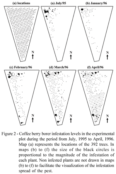
The spatio-temporal distribution of pests and diseases in fruits of perennial agricultural systems could be modelled in a similar way as for geographical variation of disease rates in human epidemiology. Each plant can be considered as equivalent to a small area or district, with the total number of fruits of that plant corresponding to its population under risk, while the number of affected fruits corresponds to the number of diseased human cases. However, there is an additional complication for the application of those models to the problem considered here. Maps of the observed infestation of the borer (Figure 2) showed that, at the beginning, the process of dispersion of the pest in the field presents an aggregated spatial pattern, typical of many arthropods. Therefore, when the infestation process starts it is common to have some plants with relatively high levels of infestation while most of the other plants stay healthy with zero infested fruits. This generates a spatial pattern with a very large number of zero counts combined with few large counts and this pattern cannot be properly fitted by the usual disease mapping models.

A natural approach to model this situation is to partition the population of plants into two or more groups and to use mixture models, particularly zero inflated models. In these models, besides the counting of zeroes coming from a distribution such as Poisson, that affects a part of the population, there also exists an additional number of zeroes from individuals belonging to a group of " non susceptible" . A literature review and a discussion on a general methodology to model zero inflated count data is presented in Ridout et al. (1998), with emphasis in applications in horticulture. Some models for zero inflated data of proportions with applications to biological control assays are also presented in Vieira et al. (2000). Other recent applications of non spatial Poisson and binomial zero inflated models can be found for instance in Hall (2000) and in a Bayesian context in Angers & Biswas (2003); Rodrigues (2003) and Ghosh et al. (2006).

Very little effort has been devoted to the modelling of these zero inflated models in a spatial context. Exceptions are the papers by Agarwal et al. (2002) and Gschlößl & Czado (2006). However, we have no knowledge of models that consider zero inflated count data structured in space and time.

The Colombian Coffee Berry Borer Infestation

The Colombian National Center of Coffee Researches, CENICAFE, carried out a large study on the population dynamics and the development of sampling techniques for the coffee berry borer. As part of this project, one of us was involved with the analysis of the first ten months of evaluation (July/1995 to April/1996) of a borer infestation experiment. During this period the pest was dispersed starting from initial focuses until almost colonizing the totality of an experimental area with 2214 plants of coffee (Coffea arabica var. Colombia).

These plants were distributed in an area of approximately 0.5 ha located in the experimental station " La Catalina" in the Pereira Colombian municipality (4º45' N, 75º45' W), 1350 meters above sea level, with an average temperature of 21.6ºC, rainfall of 1978 mm/year, and sunlight of 1606 hours/year. The plot had a slope between 40% and 60%, typical of many coffee plantations of the central Colombian coffee area, and shared no boundaries with other coffee plots. The plot was selected nine months after the planting in the field when the coffee plants presented their first flowerings. The spacing among plants was of 1.5 m × 1.5 m.

The locations (coordinates X-Y) of the 2214 plants were referenced in a Cartesian plan starting from an arbitrary origin. Due to the large size of the dataset and the high computational cost required to model the information, this study considered the analysis of a representative sub-area composed of a sample of 392 plants within the available 2214.

The pest was left uncontrolled during the experimental period besides the permanent collection of ripe, overripe and dry fruits. The information considered for analysis started to be collected monthly starting in July/1995, three months after the registration of the first important flowering stage, ending in April/1996. It began with an inspection of each plant observing the presence or absence of the borer. If there was at least one fruit infested by the borer in a plant, all fruits, healthy and infested, were counted. Otherwise, the plant was simply registered as not infested (0% of infestation) and the total number of fruits was not counted. This saving of sampling effort generated the missing value problem for the estimation in our models, which is the subject of the next subsection.

Estimation of Missing Values

The total number of fruits in healthy plants had to be estimated in order to implement the spatio-temporal modelling of the infestation process. We used the multiple imputation method (Rubin, 1987) which is based on the substitution of each missing value for m > 2 values sampled from a distribution of probability that describes as best as we can the data generating mechanism of the true unknown and missing values. With the m imputations for each missing value, it is possible to create m complete datasets and each of them is analyzed using statistical procedures as if the imputed data were real. Next, we summarize in some way the inferences from the m analyzes in each complete dataset undertaken to represent the final inference for the original dataset.

In a Bayesian context, these imputations are obtained through the usual Bayesian predictive distribution by treating the missing data as extra parameters to be estimated. We chose the multiple imputation technique because it is simple to be implemented and the missing data prediction is made separately from the infestation risk modelling. It makes possible the subsequent analysis of the complete spatio-temporal datasets.

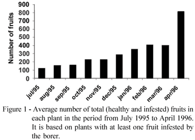
An initial analysis made of the total number of fruits on those plants where this information was collected, detected an increasing trend over time of the number of fruits (Figure 1). Considering the months of March and April of 1996, we found no evidence of significant spatial dependence between the total number of fruits on each plant. We chose these two particular months because that was when most of the plants (58% and 70%, respectively) had their total number of fruits counted. The absence of spatial correlation was verified through the calculation of the Moran's index (Moran, 1948). These two aspects motivated the model specification, as we explain next.

We assumed that the total number N_it of fruits of the i-th tree in month t followed a Poisson distribution with expected value µ_it and the counts were independently conditioned on their means. To allow for the temporal increase of N_it and heterogeneity between trees, we adopted a log-linear model with a specific intercept and growth trend for each plant. In other words, we assumed that

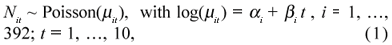
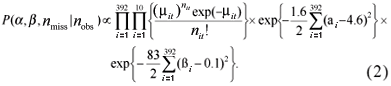
where α_i represents the overall mean of N_i0, the total number of fruits of the i-th plant at t = 0 and the parameter β_i is the growth rate of µ_it. Additionally, we assumed that, a priori, the parameters α₁ , ... , α₃₉₂ and β₁ , ... , β₃₉₂ are independent and normally distributed, with α_i ~ Normal(λ_α , τ_α) and β_i ~ Normal(λ_β , τ_β). The parameters of these priors were assumed to be λ_α = 4.6, τ_α = 1.6, λ_β = 0.1, and τ_β = 83, where τ_α and τ_β correspond to the precision (inverse of the variance) of each normal distribution.

These values were based on previous knowledge of the expected number of fruits at different plant ages. For instance, for the intercept α_i, it was assumed that a plausible value to represent the overall mean of the number of fruits at t = 0 would be 100 fruits (that is, ln(100) = 4.6), but this value could vary between a minimum of four fruits and a maximum of 2500 fruits. So, in a logarithmic scale, the width between the average and the ends (|7.8 – 4.6| = |4.6 – 1.4| = 3.2) would be approximately equal to four times the standard deviation (that is, 3.2 = 4σ), giving a precision τ = 1/ σ² = 1.6. A similar reasoning provides the values for the prior distribution for β_i.

Using Bayes theorem it is possible to use the observed data n_obs to update the knowledge on the vector of parameters (α₁ , ... , α₃₉₂ , β₁ , ... , β₃₉₂), as well as on the missing data n_miss. This updating is expressed by the joint posterior probability distribution f(α, β, n_miss | n_obs) which is proportional to

The updating was made numerically via simulation through Markov chain Monte Carlo methods (MCMC). A Gibbs sampling algorithm (Gelfand & Smith, 1990) was used to generate a sample of the posterior distribution of the parameters of interest. The method was implemented through the software WinBUGS version 1.3 (Spiegelhalter et al., 2000). Only one Markov chain of the Gibbs sampler was generated, with a pre-convergence cycle (burn-in) of 5000 iterations, following by 25000 iterations, of which we kept one in every five, giving 5000 values for the calculation of the posterior statistics of interest. The convergence of the simulations was tested following several criteria through the program CODA version 0.3 (Best et al., 1996).

The model for equations (1) and (2) was implemented ten times, using different groups of initial values to form m = 10 groups of imputed values, that represent a distribution of plausible values of the missing total number of fruits in each plant, at every time. The imputed values were the last Gibbs sampler iteration values for n_miss, and not their posterior mean, to account for the sampling variability on the true and unknown values to be predicted.

Space-time Modelling

Because the first seven evaluation months (from july/95 to january/96) had low infestation levels, with a great number of plants with completely healthy fruits (see Figure 2), it was decided to restrict the spatio-temporal analysis to the last four months (from january/96 to april/96), which summarize the period of fastest dispersion of the pest in the experimental area, starting from localized focuses at low infestation levels.

Let n_it and y_it be the total and infested number of fruits observed in plant i = 1,..., 392 and time t = 1,..., 4, respectively. We assume that the number of infested fruits, Y_it, follows a binomial distribution with parameters n_it and π_it with a logistic link function, logit (π_it) = η_it. To describe the temporal trend in the infestation rates we followed Assunção et al. (2001), using as linear predictor polynomials of first (η_it = δ_i + γ_i t), or second order (η_it = δ_i + γ_it + ν_it² ).

For the linear trend model, the parameter γ_i determines how the levels of infestation of the borer in each plant change over time. The posterior distribution of these parameters, perhaps summarized by the posterior mean, allows for spatial visualization of regions with different regimes such as increasing, stationary or decreasing infestation rates. For the models with a quadratic term, the growth rate is not constant in time, with its acceleration determined by ν_i. As models for time series, polynomial growth models are just a crude approximation. However, given the small number of time points for each plant, there were not enough measurements to experiment more sophisticated models.

The coefficients δ_i , γ_i , and ν_i of the growth models are random effects at the plant level, allowing for space-time interactions, that is, each plant has its own temporal regime of the infestation rate, and therefore, the temporal trend is possibly different for different plants. Several alternatives were considered to model these random effects a priori, as summarized in Table 1. The simplest choice is to assume a priori that all of random effects are distributed independently with a normal distribution with mean zero and unknown variance (models 1 and 5 of Table 1), that is, to assume that a priori the risk of infestation occurs independently among the plants.

A second option is to consider that neighboring plants tend to have similar values for the infestation risk. For that, we assume a conditional autoregressive Gaussian prior (CAR) for the random effects (Besag et al., 1991). If θ stands for any of the random effects, the CAR prior assumes that θ_i | θ_–i ~ Normal r , where θ_–i is the vector of all θ 's excluding θ_i, is the average of θ 's in the neighborhood ∂_i of each plant i, and r_i is the number of those neighbors. Due to risk factors spatially shared but unmeasured, we expect a random effect θ_i to be centered around the values of its neighbors θ_j. This prior spatial dependence can be induced only on the intercept of the model (models 3 and 6 of Table 1), only on the random effects that are interacting with time (models 2 and 7) or in all coefficients of the model (models 4 and 8). For each random effect with spatial dependence there is a global, fixed effect with a " flat" prior distribution. This parameterization is necessary to ensure that the models are identifiable because the CAR prior is improper (for details, see Best et al., 1999).

For the spatial random effects, we adopted a second order neighborhood as described in Besag (1974). This choice was based on results of a preliminary work of spatial modelling of the infestation of the coffee berry borer, where different neighborhood schemes were evaluated (for details, see Ruiz et al., 2003). Each of the eight models shown on Table 1 was fitted ten times, one for each imputed complete dataset. The MCMC procedure generated one chain of 30000 iterations, of which we kept 5000 (one in every five) for the calculation of the posterior statistics of interest, after discarding the first 5000 iterations. Combined posterior estimates for each parameter of interest were obtained as the arithmetic mean of the ten replications of the posterior estimates obtained for each model. The convergence of the chains was tested with the same criteria used for the missing data analysis.

Model Selection

The expected predictive deviance (EPD) criterion (Gelfand & Ghosh, 1998) was adopted to choose between the different models. This criterion considers the creation of a new dataset from the predictive distribution

f (Y_it.new | Y_it) = ∫ f (Y_it.new | π_it) f (π_it| Y_it) dπ_it,

where Y_it.new is a replicate of the observed data Y_it. This replicate was obtained sampling binomial random variables Y_it.new, conditionally on π_it values extracted from their posterior distribution. The choice of the best model is made comparing the posterior expectation of the discrepancy between the observed and predicted data through a loss function L(Y_new, Y). This posterior mean gives the EPD for each model considered. A quadratic loss function L(Y_new, Y) = (Y_new –Y)'(Y_new – Y) was used, as suggested by Laud & Ibrahim (1995), but other discrepancy functions are equally plausible.

The EPD can be expressed as the sum of two terms EPD = GM + PM as shown in Gelfand & Ghosh (1998). The GM term is a goodness of fit measure that is essentially a likelihood ratio statistic (Xia & Carlin, 1998), while the PM term is a penalty factor that penalizes very complex models. The smaller the value of EPD, the better fitted is the model.

RESULTS AND DISCUSSION

Results of the Space-time Modelling

We consider initially the first four models of Table 1, which assume a linear infestation rate for each plant. The infestation level is determined by the parameter η_it = δ_i + γ_i t for models 1 and 3 and η_it = δ_i + (ξ + γ_i)t for models 2 and 4, which breakdown the pattern into a plant-specific constant infestation rate δ_i and a temporal effect represented by the parameter γ_i. The first row of maps in Figure 3 shows the Bayesian estimates of the parameter g_i given by the posterior means obtained through the MCMC procedure applied to the observed dataset. There is a clear difference between models 2 and 4, which assumed a spatial structure for the parameter γ_i, and models 1 and 3, which did not. One striking difference is that models 1 and 3 predicted a spatial pattern that was not well defined, alternating plants with positive and negative values of . Models 2 and 4, with spatial structure on γ_i, showed a clear growth trend in the infestation levels in the Eastern side of the map and of a decrease for the Northwest area. This is reflected on the observed pattern by Eastern plants starting in a relatively high infestation level η but, as times passes, the negative γ's in this region bring this relatively high level towards smaller levels. In contrast, plants on the Northeastern part of the plot start with a low infestation level η but their positive γ's lead to continual increase with respect to their initial values. This general behavior is similar to the pattern shown by the observed data, presented in the Figure 2. In fact, the borer infestation started in the Northwest area and spread towards the East until almost all region was colonized in April/1996. However, the initial infestation in the Northeastern area decreases its relative incidence as the time passes. Another aspect that differentiates models 1 and 3 from models 2 and 4 is that the first two had 130 and 122 plants, respectively, with > 1, while + > 1 only for three and six plants in models 2 and 4, respectively. Values larger than 1 indicate an extremely fast increase that we think is not really reasonable in practice. Because of these aspects, we believe that models with spatially structured infestation rates reproduce better the observed pattern than models with spatially unstructured parameters.

Consider now models 5 to 8 which have a variable infestation rate due to the quadratic term t² with coefficient ν_i. More specifically, the infestation rate is given by γ_i + ν_it and therefore changes in time. As before, the results for spatially structured γ_i in models 7 and 8 are quite different from models 5 and 6, where γ_i had no spatial structure. Similar behavior was observed for the parameter ν (see Figure 3).

More formally, the EPD statistics to compare these eight models is presented in Table 2. The first four models, with constant infestation rate, clearly have a poorer performance as compared to the last four models. Furthermore, under this criterion the models with spatially unstructured parameters are slightly better than their spatial correspondents. It should be noted that all models had similar PM penalization factors with the GM goodness of fit factor being responsible for the differences between them.

However, models of Table 1 have a major drawback. As stated above, they are not able to model appropriately the number of not infested plants during the pest diffusion. Compared to what is predicted by these models, there is an excessively large number of zero infested fruits in the observed data (Table 3). This is especially true during the first two months of the infestation. An alternative modelling strategy is to use mixture models, such as zero inflated models, that allow for model infestation discontinuities and discriminate between infested and not infested plants, giving a specific probability model for each group of plants. Given that none of the models in Table 1 was able to capture this over dispersion, we avoid a detailed discussion of further aspects of the estimated (linear and quadratic) models at this point and postpone it to later, when we present the results of the mixture modelling approach, which is pursued next.

The Mixture Model

All coffee plant fruits in a not infested area can be attacked by the insect but, in practice, factors such as the aggregated character of the pest, small differences in microclimate inside the plantation, fertility gradients, and plants at the plot borders and close to areas already infested can make some plants more attractive than others for the borer at the beginning of the infestation. These differences between plants are likely to decrease as the pests spread and colonize the plantation. Therefore, we consider a mixture model where a proportion p_t of the plants at every time t, (t = 1, 2, 3, 4) is not attractive to the borer while the remaining proportion 1 – p_t has some infestation risk. The number of infested fruits in the attractive sub-population follows a binomial distribution with parameters n_it and π_it. Realizations of this model can generate a larger number of zero counts than a plain binomial model.

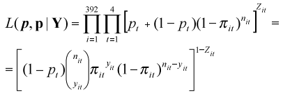
Consider the binary indicator variable Z_it, assuming the values Z_it = 1, if the plant i is not attractive to the borer at time t, and Z_it = 0, if the plant i has a positive infestation risk at time t. Therefore, Z_it ~ Bernoulli(p_t). Given that Z_it = 1 we have Y_it = 0 while if Z_it = 0 we have Y_it with binomial distribution. The marginal distribution of Y_it is called a zero inflated binomial distribution and it is given by:

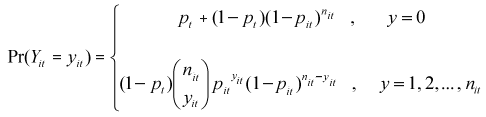
with 0 < p_t < 1. When p_t = 0, this model reduces to the standard binomial distribution. The likelihood function for that mixture model is given by the expression

We assumed that the prior distribution for the parameter p_t was an independent beta distribution (a_t, b_t), t = 1, 2, 3, 4, with a_t = b_t =1 for every t. The choice of this prior was based on previous results obtained for the purely spatial case by Ruiz et al. (2003). They evaluated the effect of the choice of different values for the hiper-parameters a_t and b_t of the prior beta distribution on the classification of the observations in each one of the components of the mixture, without finding apparent differences between not informative and highly informative priors.

A logistic link function was used for the binomial distribution. The linear predictor h_it was modelled in a similar way as for the models with the best performance found in the previous section (i.e., models 1 and 5). Hence, we analyzed two models, one with a linear trend (η_it = δ^*_i + γ^*_i t), and one with a quadratic trend (η_it = δ^*_i + γ^*_it + ν^*_it²) for the infestation rate. No spatial dependence was assumed a priori and therefore δ^*_i ~ Normal (µ^*_δ , τ^*_δ), γ^*_i ~ Normal (µ^*_γ , τ^*_γ) and ν^*_i ~ Normal (µ^*_ν , τ^*_ν). We adopted uninformative fully specified hyper-priors: µ^*_δ ~ normal (0 , 1.0E-6), τ^*_δ ~ gamma (0.001 , 0.001), µ^*_γ ~ normal (0 , 1.0E-6), τ^*_γ ~ gamma (0.001 , 0.01), µ^*_ν ~ normal (0 , 1.0E-6) e τ^*_ν ~ gamma (0.001 , 0.001).

We generated a chain of 20000 iterations of the MCMC procedure discarding the first 5000 and keeping one out of every 15 from the remaining 15000. This produced a sample of 1000 values for the parameters. The convergence of the simulations was tested following the same criteria of the previous models. As before, each model was implemented ten times to obtain combined estimates of the parameters of interest based in the ten groups of imputed values previously generated. The mixture models allowed taking into account the excess of zeroes at the levels of infestation of the first months (Table 4). These results showed a much better fit of the mixture models to the infested/healthy classification than the models without mixture evaluated previously (Table 3). Concerning the global fit of the model, Table 5 shows the EPD statistics for the mixture models. Once again the mixture models had a better fit than their homologous without mixture (Table 2). Therefore, the best model corresponded to that with two mixed populations, of attractive and non-attractive plants, and with a plant-specific quadratic infestation rate.

CONCLUSIONS

The dispersion of the infestation of the coffee berry borer had been previously modelled by Ruiz et al. (2003) ignoring the time, by considering only spatial approaches fitted to one month (March/1996), the best fitted model being then replicated in the other time periods. This is clearly, a crude way to analyze the infestation spread and the present study introduces a more elaborate and integrated way to carry out this task. We found that the mixture component is crucial in the spatio-temporal infestation of the pest, perhaps representing environmental heterogeneity in the borer habitats.

Mixture Bayesian hierarchical models allow the incorporation of covariates and random effects with and without spatial dependence. In this work, covariates possibly associated to spatial or temporal differences in the incidence of the berry infestation were not available. In future experiments it will be important to collect information on environmental covariates to explain better the phenomenon under study. The best performance of the mixture models in terms of fitting, compared to the models based in just a standard distribution, emphasize the importance of considering the excess of zeroes at the beginning of the infestation for modelling properly the estimates of the risk. Additional maps illustrating the posterior mean of the infestation risk for all of the adjusted models, as well as the WinBugs routines, can be found at the address http://www.lce.esalq.usp.br/clarice/scientia_agricola.

ACKNOWLEDGMENTS

To the National Center of Coffee Researches (CENICAFE, Colombia) for supplying the data on infestation of the coffee berry borer. The second and third authors were partially supported by CNPq.

Received October 18, 2007

Accepted May 14, 2008

• AGARWAL, D.P.; GELFAND, A.E.; CITRON-POUSTY, S. Zero-inflated models with application to spatial count data. Environmental and Ecological Statistics, v.9, p.341-355, 2002.
• ANGERS, J.F.; BISWAS, A. A Bayesian analysis of zero-inflated generalized Poisson model. Computational Statistics and Data Analysis, v.42, p.37-46, 2003.
• ASSUNÇÃO, R.M.; REIS, I.A.; OLIVEIRA, C.L. Diffusion and prediction of Leishmaniasis in a large metropolitan area in Brazil with a Bayesian space-time model. Statistics in Medicine, v.20, p.2319-2335, 2001.
• BESAG, J. Spatial interaction and the statistical analysis of lattice systems (with discussion). Journal of the Royal Statistical Society, Series B, v.36, p.192-236, 1974.
• BESAG, J.; YORK, J.C.; MOLLIÉ, A. Bayesian image restoration with two applications in spatial statistics (with discussion). Annals of the Institute of Statistical Mathematics, v.43, p.1-59, 1991
• BEST, N.; COWLES, M.K.; VINES, K. CODA: Convergence diagnosis and output analysis software for Gibbs sampling output: version 0.30. Cambridge: Cambridge University Press, 1996. 41p.
• BEST, N.G.; ARNOLD, R.A.; THOMAS, A.; WALLER, L.A.; CONLON, E.M. Bayesian models for spatially correlated disease and exposure data. In: BERNARDO, J.M.; BERGER, J.O.; DAWID, A.P.; SMITH, A.F.M. (Ed.) Bayesian statistics 6 Oxford: Oxford Science, 1999. p.131-156.
• BREWSTER, C.C.; ALLEN, J.C. Spatiotemporal model for studing insect dynamics in large-scale cropping systems. Environmental Entomology, v.26, p.473-482, 1997.
• CHEN, H.; STRATTON, H.H.; CARACO, T.B.; WHITE, D.J. Spatiotemporal bayesian analysis of lyme disease in New York State, 1990-2000. Journal of Medical Entomology, v.43, p.777-784, 2006.
• GELFAND, A.E.; GHOSH, S.K. Model choice: a minimum posterior predictive loss approach. Biometrika, v.85, p.1-11, 1998.
• GELFAND, A.E.; SMITH, A.F.M. Sampling-based approaches to calculating marginal densities. Journal of the American Statistical Association, v.85, p.398-409, 1990.
• GIBSON, G.J.; AUSTIN, E.J. Fitting and testing spatio-temporal stochastic models with application in plant epidemiology. Plant Pathology, v.45, p.172-184, 1996.
• GHOSH, S.K.; MUKHOPADHYAY, P.; LU, J.C. Bayesian analysis of zero-inflated regression models. Journal of Statistical Planning and Inference, v.136, p.1360-1375, 2006.
• GSCHLÖßL, S.; CZADO, C. Modelling count data with overdispersion and spatial effects. Statistical Papers, v.49, p.531-552, 2006.
• HALL, D.B. Zero-inflated poisson and regression with random effects: a case study. Biometrics, v.56, p.1030-1039, 2000.
• HOETING, J.A.; LEECASTER, M.; BOWDEN D. An improved model for spatially correlated binary responses. Journal of Agricultural, Biological and Environmental Statistics, v.5, p.102-114, 2000.
• HUFFER, F.W.; WU, H. Markov Chain Monte Carlo for autologistic regression models with application to the distribution of plant species. Biometrics, v.54, p.509-517, 1998.
• JARAMILLO, J.; BORGEMEISTER, C.; BAKER, P. Coffee berry borer Hypothenemus hampei (Coleoptera: Curculionidae): searching for sustainable control strategies. Bulletin of Entomological Research, v.96, p.223-233, 2006.
• KLEINSCHMIDT, I.; SHARP, B.; MUELLER, I.; VOUNATSOU, P. Rise in malaria incidence rates in South Africa: a small-area spatial analysis of variation in time trends. American Journal of Epidemiology, v.155, p.257-264, 2002.
• KNORR-HELD, L. Bayesian modelling of inseparable space-time variation in disease risk. Statistics in Medicine, v.19, p.2555-2567, 2000.
• KNORR-HELD, L.; BESAG, J. Modelling risk from a disease in time and space. Statistics in Medicine, v.17, p.2045-2060, 1998.
• LAUD, P.W.; IBRAHIM, J.G. Predictive model selection. Journal of the Royal Statistical Society, Series B, v.57, p.247-262, 1995.
• LE PELLEY, R.H. The pests of coffee London: Longmans Green, 1968. 590p.
• MABASO, M.L.H.; VOUNATSOU, P.; MIDZI, S.; DA SILVA, J.; SMITH, T. Spatio-temporal analysis of the role of climate in inter-annual variation of malaria incidence in Zimbabwe. International Journal of Health Geographics, v.5, p.1-9, 2006.
• MORAN, P.A.P. The interpretation of statistical maps. Journal of the Royal Statistical Society, Series B, v.10, p.243-251, 1948.
• NOBRE, A.A.; SCHMIDT, A.M.; LOPES, H.F. Spatio temporal models for mapping the incidence of malaria in Pará. Environmetrics, v.16, p.291-304, 2005.
• PICKLE, L.W. Exploring spatio-temporal patterns of mortality using mixed effects models. Statistics in Medicine, v.19, p.2251-2263, 2000.
• RIDOUT, M.S.; DEMÉTRIO, C.G.B.; HINDE, J. Models for count data with many zeros. In: INTERNATIONAL BIOMETRIC CONFERENCE, 19., Cape Town, 1998. Proceedings Cape Town: International Biometric Society, 1998. p.179-192.
• RODRIGUES, J. Bayesian analysis of zero-inflated distributions. Communications in Statistics, v.32, p.281-289, 2003.
• RUBIN, D.B. Multiple imputation for nonresponse in surveys. New York: John Wiley, 1987. 258p.
• RUDD, W.G.; GANDOUR, R.W. Difussion model for insect dispersal. Journal of Economic Entomology, v.78, p.295-301, 1985.
• RUIZ, R.; URIBE, P.T.; RILEY, J. The effect of sample size and spatial scale on Taylor's power law parameters for the coffee berry borer (Coleoptera: Scolytidae). Tropical Agriculture, v.77, p.249-261, 2000.
• RUIZ, R.; DEMÉTRIO, C.G.B.; ASSUNÇÃO, R.M.; LEANDRO, R.A. Modelos hierárquicos Bayesianos para estudar a distribuição espacial da infestação da broca do café em nível local. Revista Colombiana de Estadística, v.26, p.1-24, 2003.
• SPIEGELHALTER, D.; THOMAS, A.; BEST, N. WinBUGS: version 1.3; user manual. Cambridge: Cambridge University Press, 2000. 35p.
• SUN, D.; TSUTAKAWA, R.K.; KIM, H.; HE, Z. Spatio-temporal interaction with disease mapping. Statistics in Medicine, v.19, p.2015-2035, 2000.
• VIEIRA, A.M.C.; HINDE, J.; DEMÉTRIO, C.G.B. Zero-inflated proportion data models applied to a biological control assay. Journal of Applied Statistics, v.27, p.373-389, 2000.
• WALLER, L.A.; CARLIN, B.P.; XIA, H.; GELFAND, A.E. Hierarchical spatio temporal mapping of disease rates. Journal of the American Statistical Association, v.92, p.607-617, 1997.
• WINDER, L; ALEXANDER, C.J.; HOLLAND, J.M.; WOOLLEY, C.; PERRY, J. Modelling the dynamic spatio-temporal response of predators to transient prey patches in the field. Ecology Letters, v.4, p.568-576, 2001.
• XIA, H.; CARLIN, B.P. Spatio-temporal models with errors in covariates: mapping Ohio lung cancer mortality. Statistics in Medicine, v.17, p.2025-2043, 1998.
• ZHU, J.; HUANG, H.C.; WU, J. Modeling spatial-temporal binary data using Markov random fields. Journal of Agricultural, Biological, and Environmental Statistics, v.10, p.212-225, 2005.

Publication Dates

• Publication in this collection
  13 Feb 2009
• Date of issue
  Feb 2009

History

• Received
  18 Oct 2007
• Accepted
  14 May 2008