Bayesian analysis of autoregressive panel data model: application in genetic evaluation of beef cattle

Análise Bayesiana do modelo auto-regressivo para dados em painel: aplicação na avaliação genética de bovinos de corte

STATISTICS

Bayesian analysis of autoregressive panel data model: application in genetic evaluation of beef cattle

Análise Bayesiana do modelo auto-regressivo para dados em painel: aplicação na avaliação genética de bovinos de corte

Fabyano Fonseca e Silva^I,III,*; Thelma Sáfadi^II; Joel Augusto Muniz^II; Guilherme Jordão Magalhães Rosa^III; Luiz Henrique de Aquino^II; Gerson Barreto Mourão^IV; Carlos Henrique Osório Silva^I

^IUFV - Depto. de Estatística, 36570-000 - Viçosa, MG - Brasil

^IIUFLA - Depto. de Ciências Exatas, 37200-000 - Lavras, MG - Brasil

^IIIUniversity of Wisconsin - Animal Science, Madison, WI - USA

^IVUSP/ESALQ - Depto. de Zootecnia, C.P. 09 - 13418-900 - Piracicaba, SP - Brasil

ABSTRACT

The animal breeding values forecasting at futures times is a relevant technological innovation in the field of Animal Science, since its enables a previous indication of animals that will be either kept by the producer for breeding purposes or discarded. This study discusses an MCMC Bayesian methodology applied to panel data in a time series context. We consider Bayesian analysis of an autoregressive, AR(p), panel data model of order p, using an exact likelihood function, comparative analysis of prior distributions and predictive distributions of future observations. The methodology was tested by a simulation study using three priors: hierarchical Multivariate Normal-Inverse Gamma (model 1), independent Multivariate Student's t Inverse Gamma (model 2) and Jeffrey's (model 3). Comparisons by Pseudo-Bayes Factor favored model 2. The proposed methodology was applied to longitudinal data relative to Expected Progeny Difference (EPD) of beef cattle sires. The forecast efficiency was around 80%. Regarding the mean width of the EPD interval estimation (95%) in a future time, a great advantage was observed for the proposed Bayesian methodology over usual asymptotic frequentist method.

Key words: MCMC, time series forecasting, prior comparison, predictive distribution

RESUMO

A previsão dos valores genéticos de animais em tempos futuros constitui importante inovação tecnológica para a área de Zootecnia, uma vez que possibilita planejar com antecedência o descarte ou a manutenção de animais no rebanho. No presente estudo considerou-se uma análise Bayesiana de modelos auto-regressivos de ordem p, AR(p), para dados em painel, de forma a utilizar a função de verossimilhança exata, a análise de comparação de distribuições a priori e a obtenção de distribuições preditivas de dados futuros. A metodologia utilizada foi testada mediante um estudo de simulação usando a priori hierárquica Normal multivariada-Gama inversa (modelo 1), a priori independente t-Student Gama inversa (modelo 2) e a priori de Jeffreys (modelo 3). As comparações entre os modelos, realizadas por meio do Pseudo-Fator de Bayes, indicaram uma superioridade do modelo 2 em relação aos demais. Realizou-se uma aplicação em resultados reais referentes as DEP de touros da raça Nelore, sendo que, em média, a eficiência de previsão dos valores de DEP para um ano futuro foi próxima de 80%. Constatou-se considerável vantagem da metodologia proposta em relação a metodologia frequentista usual, uma vez que a implitude dos intervalos de credibilidade de 95% foram muito menores que aquelas apresentadas pelos intervalos de confiança assintóticos.

Palavras-chave: MCMC, previsão em séries temporais, comparação de prioris, distribuição preditiva

Introduction

The advantage of simultaneously modeling several time series, also called panel data analysis, is the possibility of generating more accurate predictions for individual outcomes by pooling the data rather than generating predictions of individual outcomes using the data on the individual series only. The pooling takes place because the parameters of all time series are assumed to arise from the same distribution (Liu and Tiao, 1980). The convenience in the specification of this distribution indicates that the Bayesian procedure has a theoretical advantage over the frequentist approaches, since panel data analysis is directly related to prior information.

A commonly used subjective prior distribution for parameters of auto-regressive models of order p, AR(p), is a multivariate normal, but other distributions have also been suggested such as the multivariate Student's t (Barreto and Andrade, 2004) and independent rescaled beta distribution (Liu and Tiao, 1980), in addition to non-informative prior (Sun and Ni, 2003). Thus, the choice of a prior distribution is a relevant topic in the analysis of autoregressive panel data models.

Often, only an approximate likelihood function is attempted in the Bayesian analysis of AR(p) models, because the unconditional or exact function does not provide posterior conditional distributions with closed form. The condi tionality for p initial observations in AR(p) panel data model, defined by the order p of each series, represents a larger information loss, and although the exact likelihood function increases the analysis complexity, it may still be recommended (Liu and Tiao, 1980). The Bayesian analysis of time series panel data models generates forecasts by combining all the information and sources of uncertainty into a predictive distribution for future values. The interval estimation process inherent to this distribution is theoretically more precise than those obtained from frequentist methods, in which asymptotic approximations are indiscriminately used. To illustrate this fact, we will discuss an application in the field of animal breeding.

Expected Progeny Difference (EPD) is an estimate of the individual's genetic merit for producing future progeny. EPD values are usually reported in the same measurement unit as the trait, and represent the solutions for additive genetic random effects in the Mixed Model Equations proposed by Henderson (1984). These values are published annually by the Sire Summaries, and may change from year to year; thus, several sires with EPD published in several years make up a panel data structure. In practice, to obtain EPD values in a future year for a given sire, the method used is a frequentist approach given by a 95% confidence range (CR), also called the possible chance (PC) interval defined as (Bourdon, 2000): CR_95% - EPD_a ± 1.96, where: EPD_a is EPD calculated in the current year, ACC is the accuracy of EPD_a and is the estimated genetic variance. The ACC value ranges from 0 to 1, and it informs the reliability of an EPD for a particular animal. In other words, ACC is a measure of the risk associated with the genetic estimate given by: ACC = , where PEV is the prediction error variance.

In this manuscript we propose a full Bayesian analysis of an autoregressive, AR(p), panel data model, which can be used to provide narrow estimate intervals for EPD values in one future time. The methodology considers an exact likelihood function, comparative analysis of prior distributions and predictive distributions of future observations. This methodology was evaluated by a simulation study using three priors: hierarchical Multivariate Normal-Inverse Gamma (model 1), independent Multivariate Student's t Inverse Gamma (model 2) and Jeffrey's (model 3). Model comparisons were performed using the Pseudo-Bayes Factor. An application was performed on real data from Nellore sires Expected Progeny Difference (EPD), observed during a six year period (2003-2008).

Material and Methods

Let y_it denote m time series realizations, i = 1,2,...,m, with time index given by t =1,2,...,n_i. An autoregressive AR(p) panel data model can be described as (Liu and Tiao, 1980):

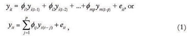
where: y_it is the actual value of a stochastic process; y_i(t-1), y_i(t-2), ... , y_i(t-p) represent values assumed in the past, Ø_i1, Ø_i2, ..., Ø_ip are autoregressive coefficients for each individual; and e_it is a non-observable error term, assumed as .

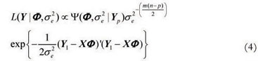
The exact likelihood function for model (1) is given by:

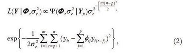
where:

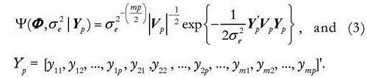
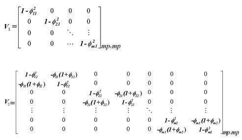
The matrix V_p is obtained by the Yule-Walker equation (Box et al., 1994). Here, we generalized this matrix for panel data using the block diagonal structure, which is illustrated for the AR(1) and AR(2) autoregressive models, respectively:

The likelihood function (2) can be written in matrix notation as:

where:

Y₁ = [y_1p+1, y_1p+2, ..., y_1n , y_2p+1 ,y_2p+2, ..., y_2n, ..., y_{mp +1}, y_mp+2, ..., y_mn]'_{m(n-p) x 1} ,

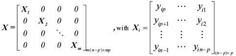
and,

An important issue with the Bayesian implementation of the AR(p) model refers to the prior specification, because the use of an inappropriate prior may lead to elevated fluctuations in the parameter estimates (Kass and Raftery, 1995). The hierarchical multivariate Normal - Inverse Gamma prior (model 1), independent multivariate Student's t - Inverse Gamma prior (model 2), and the Jeffrey's prior (model 3).

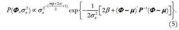
In the case of a hierarchical multivariate Normal- Inverse Gamma prior, we have:

P(Φ ,) = P(Φ|) P() , with Φ| ~ N(µ,P), with and ~ IG(α,β), such that:

and 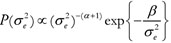, leading to the following joint prior distribution:

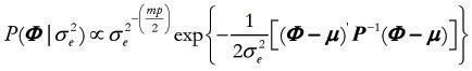
The independent multivariate Student t Inverse Gamma prior is givem by: P(Φ ,) P(Φ)P() in which Φ ~Mult. Student t (µ, P), with υ degrees of freedom, and ~ IG(α,β), such that: 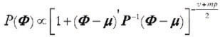. The resulting joint prior distribution is then:

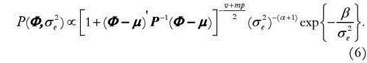
The componentsµ, P, α and β in the expressions 5 an 6 are hyperparameters, whose values must be specified. An alternative for prior specification is the use of a non-informative prior, which represents the lack of knowledge when a certain parametrical family is chosen. Jeffrey's prior approach to autoregressive model used here was presented by Broemiling and Cook (1993), which is given by: .

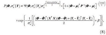
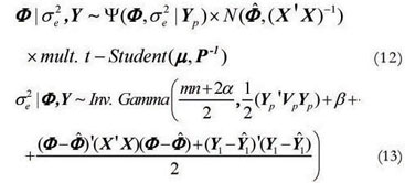
Under the Bayesian approach, the prior beliefs about parameters are updated with the information from the data to produce the posterior distribution of the parameters. Thus, it summarizes the current state of knowledge about all the uncertain quantities in a model (Gelman et al., 2003). In this study, we used the same sample information, that is, the same exact likelihood function, combined with each alternative prior distribution, in order to obtain three different joint posterior distributions. Using the Bayes Theorem, , such that the resulting joint posterior distribution for each prior specification,is given by:

Model 1:

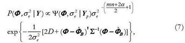
where:

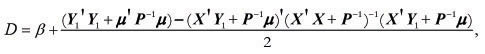
Σ = X' X + P^-1 and = (X' X + P^-1)^-1(X' Y₁ + P^-1µ).

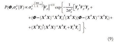
Model 2:

where:

= (X' X)^-1(X' Y₁) and ₁ = X = (X' X)^-1(X' Y₁)

Model 3:

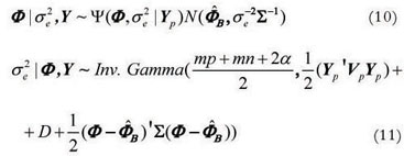
In a Bayesian analysis, the marginal posterior distributions, which contain all relevant information about the unknown parameters, are obtained by the multidimensional integration of the joint posterior distribution. These integrals are usually impossible to evaluate analytically, but Markov chain Monte Carlo (MCMC) simulation, such as the Gibbs sampler and Metropolis-Hastings, can be used instead (Gelman et al, 2003). The full conditional posterior distributions for Φ and , are necessary in order to apply MCMC. These distributions can be represented as follows:

Model 1:

Model 2:

Model 3:

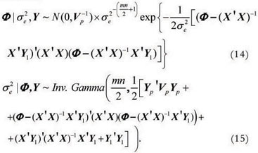
The conditional posterior distributions of have a closed form for all considered priors, which is an Inverse Gamma probability density distribution. Therefore, the Gibbs Sampler algorithm can be used to generate samples of the marginal posterior distribution. For the parameter F, however, a closed form can not be obtained, and so we used the Metroplis-Hastings algorithm.

For each prior, single chains with starting values obtained by maximum likelihood estimation were run. Although to use multiple chains is more reliable, avoiding that a single sequence is stuck in some unrepresentative small region of the parameter space, this method is not always recommended. According to Kass et al. (1998), if the convergence is very slow, as in the present study, sometimes runing just one chain can be better than several chains for correspondingly less time.

After several trials, by visual inspection of the graph, the chain length was set to 50,000 and the burn-in period 20,000 iterations, higher than the minimum burn-in required according to the Raftery and Lewis (1992) criteria. Sampling interval (thinning) was set to 3 iterations, so that a total of 10,000 samples were kept for posterior analyses. Convergence was tested for each chain separately using the Geweke (1992) criteria.

The Gibbs Sampler and Metropolis-Hastings algorithms were implemented in the R software (R Development Core Team, 2008). The mvtnorm package was used to generate random numbers of multivariate Normal and Student's t distributions, and the rinvgamma function (MCMCpack package) for the inverse Gamma distribution. The cited convergence criteria were implemented via the BOA (Bayesian Output Analysis) package (Smith, 2007).

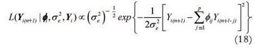
In Bayesian forecasting, the prediction of future observations are obtained by a posterior predictive distribution, which is given by a conditional distribution of future data, conditioned on past data. In the present panel data analysis, for a specific individual i, the distribution for a future observation is given by:

, where:

The term is obtained by the following model:

Y_i(n+1) = ø_i1Y_in + ø_i2Y_i(n-1) + ø_i3Y_i(n-2)+ ... + ø_ipY_i(n+1-p) + e_i(n+1), or Y_i(n+1) = ø_ijY_i(n+1-j) + e_i(n+1), assuming

that e_i(n+1)~ N (0,), such that:

Generalizing the expression (17) for m individuals, we have:

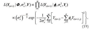
Using matrix notation, the expression (19) can be expressed as:

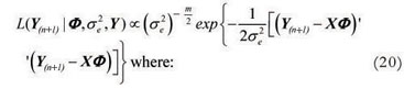
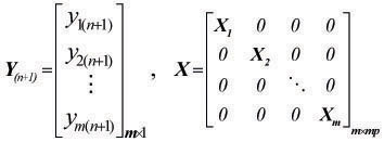and X_i = [y_iny_i(n-1) ...y_i(n+1-p)]_1xp.

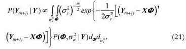
Therefore,

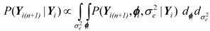
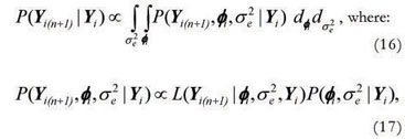
, where P(Φ,|Y)is the joint posterior distribution previously presented. Then, by the generalization of expression (16), we have that:

This integral does not present an analytical solution, but according to Heckman and Leamer (2001) it is possible to obtain an approximation via MCMC algorithm with the distribution: 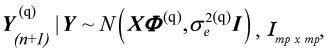, I_{mp x mp}, where I is an identity matrix. The set of values generated by this multivariate normal distribution, at each q MCMC iteration step, constitutes a sample of future observations from the posterior predictive distribution. Then, the point estimate of this value for future observations, is given by the mean of this sample (Y_(n+1)|Y).

The comparison between priors used the Pseudo-Bayes Factor (PBF) (Gelfand, 1996), which is defined as the ratio of (Y_(n+1)|Y) produced by models M_z and M_w:

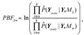
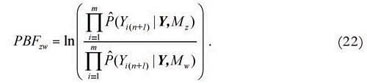
where k is the number of future time points to be predicted. If PBF_zw > 0 then M_z is selected, otherwise M_w is selected. In the present study it was assumed that k = 1, however, as the panel data structure demands a generalization for each individual series i, we have:

A simulation study was conducted to evaluate the proposed methodology. The AR(2) model was used because it is the most simple multi-parametric autoregressive approach. It is given by:

Y_it = ø_i1Y_i(t-1) + ø_i2Y_i(t-2)+ e_it; with i = 1,2,...,10, and t = 1,2,...,12,

where:

ø_i = [ø_i1,ø_i2] with ø_i1+ ø_i2< 1, ø_i1- ø_i2< 1 and -1 < ø_i2< 1 such that the series is stationary.

The parameter values, ø_i1 and ø_i2, were generated by multivariate normal (model 1) and multivariate Student's t distributions (model 2), so it is possible to assume these distributions as the true prior distributions in the efficiency analysis of the Pseudo-Bayes Factor. The distributions used to generate the parameter values for models 1 and 2 are given, respectively, by:

ø_i ~ N and ø_i ~ Mult.Student t

and

The residual distribution was Normal, e_it ~ N(0, ), were was drawn from an Inverse Gamma distribution, ~ IG(3,2).

This simulation study also provides an alternative way to evaluate the autoregressive panel data model predictive ability, which is assumed by predicting the last observation,

_il2, which was excluded from the analysis for parameter estimation.

The proposed methodology was applied to a real data set obtained from the animal breeding field, which refers to Expected Progeny Difference (EPD) for Nellore cattle. The data are from an annual genetic analysis of 117 sires and were provided by the Animal Breeding Group of the Universidade de São Paulo, in Pirassununga, state of São Paulo, Brazil. The EPD values for the weight gain from weaning (205 days of age) to 550 days of age were recorded between 2003 to 2008.

These EPD values were calculated with different accuracy levels, since these values are indicators of the reliability of the published genetic estimates for each animal. If all animals had the same accuracy level, characteristics such mean weight, age and herd, among others, could be used in order to classify latent sire groups. We split the animals into three groups according to their 2007 accuracy levels. These groups were classified as low (0 to 40%), median (41 to 60%) and high (above 60%) accuracy, which contained 31, 63 and 23 sires, respectively. These groups were constructed to ensure the homogeneity within each classification widely required for panel data analysis.

The order of the autoregressive process was identified with autocorrelogram plots, which showed that only first and second order models make sense. The AR(2) model was chosen, since this model includes the AR(1) structure.

Predictive ability was evaluated using 2008 EPD values, which were omitted from the estimated sample. To compare the forecasting precision of EPD values in one period ahead with the conventional method, we use a 95% confidence range (CR), and 95% Bayesian credible interval, which is based on 2.5 an 97.5 percentiles of the posterior predictive distribution, the mean width intervals were calculated. The point estimates from different methods were compared by through the root mean square error (RMSE).

Results and Discussion

The Bayesian methodology was efficient (Tables 1 and 2), with 95% credibility intervals containing 80% and 90% of the ø₁ parametric values, and 90% and 100% of the ø₂ parametric values, respectively for models 1 and 2. Furthermore, the estimates from model 2 also presented best agreement with the true values, since the RMSE for this model, regarding respectively ø₁ (0.0441) and ø₂ (0.0392), were smaller those obtained from model 1, respectively 0.0678 and 0.1346 for ø₁ and ø₂. These same considerations apply to residual variance estimates (Table 3).

The last three columns in Tables 1, 2 and 3 indicate that all chains give very similar results. The convergence was seemingly achieved, with the z-scores of the Geweke tests never higher than 1.96. The burn-in period values used were much higher than the minimum recommended by the procedure of Raftery and Lewis. For model 1, 60% of the credibility intervals contained the true values, and 80% for model 2 (Table 4). Thus, the joint evaluation of the two models produced an efficiency of 70%, which is similar to other studies that performed also model predictive ability evaluation. De Alba (1993) simulated independent time series with the AR(4) model and noted an efficiency of 75%, while Hay and Pettitt (2001) obtained 58% in the analysis of twelve pneumonia incidence time series using generalized the AR(1) model for count data. In relation to efficiency of point estimates, the RMSE calculated were very similar for the two models, 0.3541 and 0.3469, respectively for models 1 and 2.

Although model 2 was presented as the best for sample fit (Tables 1, 2 and 3), and the best in predictive ability (Table 4), the models were also compared by the Pseudo-Bayes Factor. The results are presented in Table 5, which show the model 2 superiority in relation to models 1 and 3, even when data were simulated using model 1. This interesting result can be in part explained by Student's t distribution with higher degrees of freedom, which is similar to the normal distribution. In general, the literature has related the Student's t prior quality for parameters of time series autoregressive models, and among these we refer the reader to Barreto and Andrade (2004).

The Pseudo-Bayes Factor values calculated to compare the three models fitted to the EPD data are presented in Table 6. The results are similar to those obtained with the simulated data, indicating a better performance for the independent multivariate Student's t - Inverse Gamma prior. The Pseudo-Bayes Factor magnitude in relation to the hierarchical multivariate Normal-Inverse Gamma is small, and the non-informative Jeffreys' prior had the worse results. This fact is very well discussed by Lambert et al. (2005), who indicate that, even if we do not have well determined information about the parameters, it is very important to use and compare the informative prior with the non-informative, because probably the informative one will lead to better posterior results.

In the context of our data, at each new sire annual evaluation the researcher can increase the amount of information coming from the data, which means that the prior information used in this Bayesian analysis can be given by the posterior distribution obtained from the previous year. Thus, after several years, as the sample size increases, the point and interval Bayesian estimates of the parameters, including the EPD for a future year, will be driven more and more by the observed data rather than by the prior. Anyway, due to the great influence of the prior information in the first step of this proposed system, the Pseudo-Bayes Factor was used to objectively choose the prior distribution, and the independent Multivariate Student's t - Inverse Gamma (model 2) was indicated. Concluding, we believe that subjective prior choice can lead to results that are driven not by the data but by prior unconfirmed beliefs and this fact may compromise the reliability of the study findings.

After the choice of the best prior, independent multivariate Student's t Inverse Gamma, the predictive ability produced by this model is shown in Table 7. It represents the percentage of sires whose credibility intervals contained the EPD true values, corresponding to year 2008. The residual variance of posterior estimates for each accuracy group is also presented in Table 6. The predictive ability of this proposed Bayesian methodology was efficient to forecast future EPD values, since the percentages were consistently high, around 80%.

The mean width of EPD interval estimation (95%) for the usual method (Bourbon, 2000) and proposed Bayesian forecasting are presented in Figure 1. These results demonstrate a great advantage of the Bayesian methodology, which provide narrow intervals for each accuracy group. In relation to efficiency of point estimates, the Bayesian method also presented more efficiency based on RMSE (0.3022 versus 0.9345).

Conclusions

The proposed full Bayesian framework for analysis of panel data, using an exact likelihood function, comparative analysis of priors and predictive distributions of future observations worked very well in our study, for both, simulated and real data sets, since the predictive ability was nearly 90% for all considered models. Comparisons by the Pseudo-Bayes Factor indicated superiority of the independent Mul

tivariate Student's t - Inverse Gamma prior in relation to the others. The real data analysis indicated the importance of grouping sires by accuracy values, and also showed a forecast efficiency around 80%.

Received September 03, 2009

Accepted August 16, 2010

• Barreto, G.; Andrade, M.G. 2004. Robust Bayesian Approach for AR(p) Models Applied to Streamflow Forecasting. Journal of Applied Statistical Science 12: 269-292.
• Bourdon, R.M. 2000. Understanding Animal Breeding. Prentice-Hall, Upper Saddle River, NJ, USA.
• Box, G.E.P.; Jenkins, G.M.; Reinsel, G.C. 1994. Time Series Analysis: Forecasting and Control. Holden-Day, San Francisco, CA, USA.
• Broemiling, D.L.; Cook, P. 1993. Bayesian estimation of the mean of an autoregressive process. Journal of Applied Statistics 20: 25-38.
• De Alba, E. 1993. Constrained forecasting in autoregressive time series models: a Bayesian analysis. International Journal of Forecasting 9: 95-108.
• Gelman, A.; Carlin, J.B.; Stern, H.S.; Rubin, D.B. 2003. Bayesian Data Analysis. Chapman and Hall, Boca Raton, FL, USA.
• Gelfand, A.E. 1996. Model Determination Using Sampling Based Methods. Chapman and Hall, London, UK.
• Geweke, J. 1992. Evaluating the accurary of sampling-based approaches to the calculation of posterior moments. Oxford University Press, Oxford, UK.
• Hay, J.L.; Pettitt, A.N. 2001. Bayesian analysis of a time series of counts with covariates: an application to the control of an infectious disease. Biostatistics 2: 433-444.
• Heckman, J.; Leamer, E. 2001. Handbook of Econometrics. Elsevier Science, Amsterdam, The Netherlands.
• Henderson, C.R. 1984. Applications of Linear Models in Animal Breeding. University of Guelph Press, Ontario, Canada.
• Kass, R.E.; Carlin, B.P.; Gelman, A.; Neal, R.M. 1998. Markov Chain Monte Carlo in practice: a roundtable discussion. American Statistician 52: 93-100.
• Kass, R.E.; Raftery, A.E. 1995. Bayes Factor. Journal of the American Statistical Association 90: 773-795.
• Lambert, P.C.; Sutton, A.J.; Burton, P.R.; Abrams, K.R.; Jones, D.R. 2005. How vague is vague? A simulation study of the impact of the use of vague prior distributions in MCMC using WinBUGS. Statistics in Medicine 24: 2401-2428.
• Liu, L.M.; Tiao, G.C. 1980. Random coefficient first-order autoregressive model. Journal of Econometrics 13: 305-325.
• R Development Core Team. 2008. R: A language and environment for statistical computing. R Foundation for Statistical Computing, Vienna, Austria.
• Raftery, A.E.; Lewis, S. 1992. How many iterations in the Gibbs sampler? Oxford University Press. Oxford, UK.
• Smith, B.J. 2007. boa: An R Package for MCMC Output Convergence Assessment and Posterior Inference. Journal of Statistical Software 21: 1-37.
• Sun, D.; Ni, S. 2003. Noninformative priors and frequentist risks of Bayesian estimators of vector-autoregressive models. Journal of Econometrics 115: 159 -197.

Publication Dates

• Publication in this collection
  31 Mar 2011
• Date of issue
  Apr 2011

History

• Received
  03 Sept 2009
• Accepted
  16 Aug 2010