Critical points in logistic growth curves and treatment comparisons

BIOMETRY, MODELING AND STATISTICS

Critical points in logistic growth curves and treatment comparisons

José Raimundo de Souza Passos; Sheila Zambello de Pinho^*; Lídia Raquel de Carvalho; Martha Maria Mischan

UNESP/IBB – Depto. de Bioestatística, C.P. 510 – 18618-970 – Botucatu, SP – Brasil

ABSTRACT

Several biological phenomena have a behavior over time mathematically characterized by a strong increasing function in the early stages of development, then by a less pronounced growth, sometimes showing stability. The separation between these phases is very important to the researcher, since the maintenance of a less productive phase results in uneconomical activity. In this report we present methods of determining critical points in logistic functions that separate the early stages of growth from the asymptotic phase, with the aim of establishing a stopping critical point in the growth and on this basis determine differences in treatments. The logistic growth model is fitted to experimental data of imbibition of araribá seeds (Centrolobium tomentosum). To determine stopping critical points the following methods were used: i) accelerating growth function, ii) tangent at the inflection point, iii) segmented regression; iv) modified segmented regression; v) non-significant difference; and vi) non-significant difference by simulation. The analysis of variance of the abscissas and ordinates of the breakpoints was performed with the objective of comparing treatments and methods used to determine the critical points. The methods of segmented regression and of the tangent at the inflection point lead to early stopping points, in comparison with other methods, with proportions ordinate/asymptote lower than 0.90. The non-significant difference method by simulation had higher values of abscissas for stopping point, with an average proportion ordinate/asymptote equal to 0.986. An intermediate proportion of 0.908 was observed for the acceleration function method.

Keywords: nonlinear regression, asymptotic regression, stopping critical level, seeds imbibition

Introduction

Biological phenomena can have a mathematically characterized behavior as a function of time with a strong increasing function in early development stages, followed by a less pronounced growth, sometimes showing stability. The separation between these phases is of great importance since, in many processes, the maintenance of a less productive phase results in an uneconomical activity. Sometimes the growth phases have different biological meanings and it is important to separate them.

Several methods have the aim to determine critical points that separate growth phases, as in Cate Jr. and Nelson (1965) to determine critical level of nutrients in plants and Portz et al. (2000) that use the segmented regression in a fish study. The segmented regression method is also used in Cate Jr. and Nelson (1971) and discussed in Rayment (2005) which named it «Linear Response and Plateau Model».

Empirical methods separate growth stages with basis in yield percentages, generally using the levels of 90 to 95 % of maximum yield as an upper limit, as in Korndörfer et al. (2001) working with rice (Oryza sativa), Evans et al. (2008) with a ornamental bush (Euonymus fortunei), and Santos et al. (2004) with alfalfa (Medicago sativa). Other statistical and mathematical methods are employed with the same aim to determine critical points in logistic curves (Carvalho and Pinho, 1996 and Mischan et al., 2011) fitted to data of seed imbibition and weight of cattle, respectively.

The aim of this paper is to determine new methods to obtain critical points in logistic growth curves and compare them with some already available in the literature, in order to offer alternatives for decisions on the best time to stop the process. We also indicate the possibility of comparing treatments through the analysis of variance of the critical points.

Materials and Methods

The statistical model of growth used is the logistic one:

with parameters α, β and γ, α > 0 and γ > 0, where y_j is the observed measure at time x_j, and e_j is the random error, with normal distribution (0, σ²). The estimated function is represented by

with a, b and c the estimates of the parameters α, β and γ, respectively. To determine the stopping critical points in the logistic model six methods are used as described below.

M₁ - Acceleration function method with point P₁ (x₁; y₁)

The method, described in Mischan et al. (2011), works with the acceleration function of the logistic model of growth, represented by its second derivative

which has two extreme points, a maximum and a minimum, and three inflection points. After the last point of inflection, called asymptotic deceleration point (P₁), the deceleration of growth is very slow and approaches to zero when x tends to infinity. The point coordinates are obtained by equating the derivative of order 4 to zero: P₁ [-(ln(5-2) + b) / c; a(3 + ) / 6] or, approximately, P₁ [(2.29 - b)/c ; 0.908a].

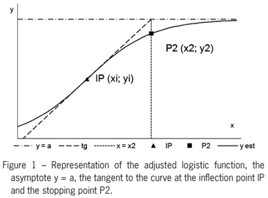
M₂ - Tangent at the inflection point method with point P₂ (x₂; y₂)

In the asymptotic growth function estimated, with an inflection point P_i (x_i; y_i), we call y'_i be the value of the first derivative of the function at its inflection point. If we consider a tangent to the curve at this point as a linear approximation to the growth phase before the asymptote, its intersection with the asymptote of the function y = a can be interpreted as an indication of maximum growth and therefore a stopping point. The equation of this tangent line is

and in its intersection with the asymptote (y = a) is

where x₂ is the abscissa of the P₂ point. Therefore,

The logistic function has P_i (-b/c; a/2) and y'_i = ac/4, hence P₂ [(2-b)/c; a/(1+exp(-2))] or, approximately, P₂ [(2-b)/c; 0.881a].

See Figure 1.

M₃ - Segmented regression method with point P₃ (x₃; y₃)

For n pairs (x_j; y_j) from the observed data the segmented regression model can be represented by two lines, one parallel to the x-axis and one inclined,

with the restriction (ρ-x_j) = 0 for j > n₁+1, where n₁ = number of observations before the intersection point of straight lines, α₁ = intersection of line with the vertical axis y, β₁ = slope, ρ = abscissa of the intersection point and e_j = experimental error. The estimates of parameters α₁, β₁ and ρ are represented by a₁, b₁ and r, respectively. The estimate r is the abscissa of the sought critical point, r = x₃.

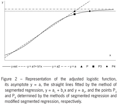
M₄ - Modified segmented regression method with point P₄ (x₄; y₄)

When determining the intersection point in the segmented regression method, this point is the beginning of the asymptotic phase of growth and is therefore a point of early occurrence. Naming the horizontal line determined in the former method y = a₂, we see that the fitted curve does not reach the asymptote y = a, but intersects the line y = a₂, a₂ < a at some point P₄, occurring later in time as compared to P₃. Based on this information, the estimate a₂ = intersection of horizontal line with the y-axis, obtained at the segmented regression method M₃, is used as the ordinate of the sought critical point. Observe that y = a₂ is the least squares straight line fitted to the data that are distributed in a nearly horizontal manner, parallel to the x-axis. These data are placed after a point P₄ (x₄, y₄), where y₄ = a₂ and x₄ is determined by the function fitted to the data in the logistic curve,

where

See Figure 2.

M₅ - Non-significant difference method with point P₅ (x₅; y₅)

The method for determining the point of non-significant difference is described in Carvalho and Pinho (1996). We consider the difference y* = a-y, between the estimated function and its asymptote, and we verify from which point we can consider it non-significant by a Student t-test. The abscissa x₅ of the critical point determined by this method is the solution of the equation

for a value of T = t_α,f, where t_α,f is the unilateral t-test at significance level α, with f = number of degrees of freedom associated with the estimate of error variance. The resolution is made with the parameter estimates, their variances and covariances, and the estimated variance of y* for x = x₅. The values of the abscissas of the points are generally beyond the range of observation data, which suggests that this method is quite strict in order to determine a stopping critical point to the observations of the experiment. This rigor can be mitigated considering a difference y* not between y and its asymptote, but between y and a percentage, p, of this. In this case we have: y* = pa - y. In this paper we adopted p = 0.90, which is considered in several articles in the literature on critical points, for example in Korndörfer et al. (2001), Evans et al. (2008) and Santos et al. (2004). This p value is very close to that determined in method M₁, 0.908.

M₆ - Non-significant difference method by simulation with point P₆ (x₆; y₆)

The proposed method for determining the critical point of stopping by simulation is based on the technique of Monte Carlo simulation (Shapiro and Gross, 1981). They also appear in literature applications of this technique in studies of sampling distribution of estimators in nonlinear regression models (Bates and Watts, 1988). In this method, after adjusting the asymptotic growth function to data, new observations of the response variable are generated and repeated 1,000 times, based on the values of the dependent variable, the estimated parameters and sample variance. Then the nonlinear regression model is fitted again to the replicates obtained by simulation. From the inflection point of each of the simulated curves, the difference D between the ordinate of the considered point and the estimated asymptote is determined. This process is repeated at a step k to a maximum allotted time for the independent variable. The empirical sampling distribution of the random variable D and the percentiles p_2.5 and p_97.5 are determined for each empirical distributions obtained previously. The stopping point P₆ (x₆; y₆) for the value of the dependent variable is the first value of p_2.5 < 0.

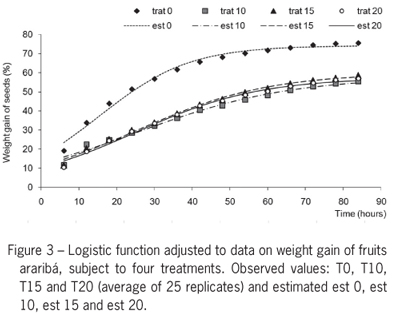
The model is fitted to data of accumulated weight gain of fruits of araribá (Centrolobium tomentosum), in percentage, during soaking for 84 h in distilled water, subjected to treatment with sulfuric acid during the times {0, 10, 15, 20 min.} represented by T0, T10, T15 and T20 as described in Carvalho and Pinho (1996). The experiment had 25 repetitions. The parameter estimates, their standard errors, confidence intervals and coefficients of asymmetry of Hougaard (1985) were determined.

In the analysis of variance of the abscissas and ordinates were considered the factors 'treatments' and 'methods of determining breakpoints' and the interaction between them. The data used in these tests is obtained by fitting the logistic function and posterior determination of breakpoints for each of the 25 replicates for four treatments.

Results and Discussion

Table 1 and Figure 3 present the results of the logistic function fit to the data of weight gain of fruits araribá for each of the four treatments, using all the replicates in each time. Table 1 shows the parameter estimates, their standard errors and approximate confidence intervals limits at 95 % and the coefficients of asymmetry of Hougaard. All parameter estimates present values of t = estimate / standard error of estimate with p-values < 0.0001. The parameters estimates of β and γ present coefficients of asymmetry less than 0.1 which, by the classification of Ratkowsky (1989), suggest how the estimators are quite close to linear. For the parameter α, the greater asymmetry coefficient was 0.231 in the treatment T10, which makes the estimator reasonably close to linear (coefficient between 0.1 and 0.25). The Durbin-Watson test to check for autocorrelation and the Breusch-Pagan for homogeneity of variances showed that the model of independent errors and constant variance can be employed.

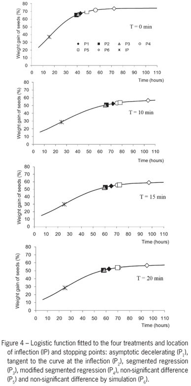
Table 2 and Figure 4 show the stopping critical points (x_i, y_i) determined by methods M₁ to M₆ for each treatment, as well as the inflection point.

The analysis of variance of estimated abscissas showed significant interaction (p < 0.001) among the factors 'treatment' and 'methods for determining the stopping points'. The M₂ (tangent at the inflection point method) and M₃ (the segmented regression method) did not differ in any treatment and had the lowest values of abscissas (Tukey, p < 0.05). Both methods assume a straight line representing the initial growth that intersects with a horizontal line representing the asymptotic growth - the asymptote (a) in the M₂ method and the least squares line of y = a₂ fitted to final growth in method M₃. The method M₆ (non-significant difference between the function and its asymptote, determined by simulation) shows breakpoints with the highest values of abscissas, x_i, differing from other methods in all treatments. Abscissa values determined by the method M₄ (modified segmented regression) are larger than those determined by the method M₃. So, the modified segmented regression method is an efficient alternative to the method of segmented regression M₃, when we want a stop point occurring later. The M₁ method (accelerating growth function) leads the points with abscissas intermediate in comparison with other methods.

The comparison between treatments showed that T10 differs from other treatments having the highest abscissa of breakpoints. T15 and T20 did not differ and T0 leads to lower values. All the treated seeds, therefore, showed a reduced growth rate compared with the control T0, what is already evident in the parameter estimates presented in Table 1, where c (T0) = 0.071, a value higher than the others. A high value for c shows that the estimated growth rate is high, which implies a smaller value for the abscissa of the breakpoint.

Analyzing the ordinate values of the breakpoints, significant main effects were found for the factors 'treatment' and 'methods' and no significant interactions. In general the differences between methods are similar to those seen in the analysis of abscissas: the smallest ordinates are obtained by methods M₂ and M₃, not showing difference among them. The method M₆ has the highest ordinate value, differing from other methods; M₁ is in the middle. If the ordinate criterion is used to compare treatments, T0 also differs from other treatments presenting, unlike the comparisons of abscissas, the highest average value; this is probably due to the high growth rate of T0 compared to the treated seeds.

The determination of a stopping point in the adjusted logistic growth curve to data from soaked seeds of araribá can be made by different methods, mathematical or statistical methods, which can be considered different regarding the values of their coordinates. The segmented regression and the tangent at the inflection point methods lead to the decision of a significant slowdown in growth from lower values of abscissa; they lead to early stopping points, in comparison with other methods, with proportions ordinate/asymptote a little lower than 0.90. The non-significant difference method by simulation determines higher values of abscissas for stopping points, with an average proportion ordinate/asymptote 0.986, a value that shows an ordinate excessively near to the asymptote. An intermediate proportion of 0.908 is obtained by the acceleration function method. The segmented regression method (M3), the acceleration function method (M1) and the modified segmented regression method (M4) are quite simple in application and cover a wide range of variation in the amounts ordinate/asymptote, on average 0.883, 0.908 and 0.941, respectively, which is very useful in practice. The method M1 depends only on a mathematical formula that uses the parameters of the fitted model, M3 is a method already widely used in literature and M4 is a simple modification of M3. On the other hand, the method of the tangent at the inflection point (M2) shows very similar results to those obtained by the method M3, segmented regression, but the points are difficult to obtain; the non-significant difference methods (M5 and M6) are not simple to apply and M6 leads to excessively high values of abscissas with ordinates very close to the asymptote. The breakpoints can also be used as a criterion for comparing treatments in experiments where the growth functions are adjusted.

Received August 01, 2011

Accepted March 13, 2012

Edited by: Thomas Kumke

• Bates, M.D.; Watts, D.G. 1988. Nonlinear Regression Analysis and Its Applications. John Wiley, New York, NY, USA.
• Carvalho, L.R.; Pinho, S.Z. 1996. Method for comparison of logistic growth curve with the presence of residual autocorrelation. Energia na Agricultura 11: 3855 (in Portuguese, with abstract in English).
• Cate Jr., R.B.; Nelson, L.A. 1965. A Rapid Method for Correlation of Soil Tests Analyses with Plant Response Data. International Soil Testing, Raleigh, NC, USA. (Technical Bulletin.North Carolina Agricultural Experiment Station, 1).
• Cate Jr., R.B.; Nelson, L.A. 1971. A simple statistical procedure for partitioning soil test correlation data into two classes. Soil Science Society of America Proceedings 35: 658659.
• Evans, R.Y.; Smith, S.J.; Paul, J.L. 2008. Nitrogen critical level determination in the woody ornamental shrub Euonymus fortunei Journal of Plant Nutrition 31: 20752088.
• Hougaard, P. 1985. The appropriateness of the asymptotic distribution in a nonlinear regression model in relation to curvature. Journal of the Royal Statistical Society, Serie B 47: 103114.
• Korndörfer, G.H.; Snyder, G.H.; Ulloa, M.; Powell, G.; Datnoff, L.E. 2001. Calibration of soil and plant silicon analysis for rice production. Journal of Plant Nutrition. 24: 10711084.
• Mischan, M.M.; Pinho, S.Z.; Carvalho, L.R. 2011. Determination of a point sufficiently close to the asymptote in nonlinear growth functions. Scientia Agricola 68: 109114.
• Portz, L.; Dias, C.T.S.; Cyrino, J.E.P. 2000. A broken-line model to fit fish nutrition requirements. Scientia Agricola 57: 601607.
• Ratkowsky, D.A. 1989. Handbook of Nonlinear Regression Models. Marcel Dekker, New York, NY, USA.
• Rayment, G.E. 2005. Statistical aspects of soil and plant test measurement and calibration in Australasia. Communications in Soil Science and Plant Analysis 36: 107120.
• Santos, A.R.; Mattos, W.T.; Almeida, A.A.S.; Monteiro, F.A.; Corrêa, B.D.; Gupta, U.C. 2004. Boron nutrition and yield of alfalfa cultivar crioula in relation to boron supply. Scientia Agricola 61: 496500.
• Shapiro, S.S.; Gross, A.J. 1981. Statistical Modeling Techniques: Statistical, Textbooks and Monographs. Marcel Dekker, New York, NY, USA.

Publication Dates

• Publication in this collection
  28 Sept 2012
• Date of issue
  Oct 2012

History

• Received
  01 Aug 2011
• Accepted
  13 Mar 2012