Spatial prediction of soil penetration resistance using functional geostatistics

ABSTRACT

Knowledge of agricultural soils is a relevant factor for the sustainable development of farming activities. Studies on agricultural soils usually begin with the analysis of data obtained from sampling a finite number of sites in a particular region of interest. The variables measured at each site can be scalar (chemical properties) or functional (infiltration water or penetration resistance). The use of functional geostatistics (FG) allows to perform spatial curve interpolation to generate prediction curves (instead of single variables) at sites that lack information. This study analyzed soil penetration resistance (PR) data measured between 0 and 35 cm depth at 75 sites within a 37 ha plot dedicated to livestock. The data from each site were converted to curves using non-parametric smoothing techniques. In this study, a B-splines basis of 18 functions was used to estimate PR curves for each of the 75 sites. The applicability of FG as a spatial prediction tool for PR curves was then evaluated using cross-validation, and the results were compared with classical spatial prediction methods (univariate geostatistics) that are generally used for studying this type of information. We concluded that FG is a reliable tool for analyzing PR because a high correlation was obtained between the observed and predicted curves (R² = 94 %). In addition, the results from descriptive analyses calculated from field data and FG models were similar for the observed and predicted values.

functional Kriging; compaction; spatial variability; functional data

Introduction

Agricultural soils behave like a complex system that accumulates and transmits air, water, nutrients and heat to microorganisms and plants (Orjuela-Matta et al., 2012). Soil penetration resistance (PR) is a good indicator of soil physical quality once it is easily measured and interpreted, and correlated with other soil attributes (Guimarães et al., 2013). The PR can be used to manage other parameters, such as crop output and water flow during rainy seasons or irrigation. Quantifying the degree of soil compression consists of measuring the PR, which indirectly measures the energy that roots need to deform the soil structure or to penetrate soil pores (Medina et al., 2012).

The study of soil properties in agricultural zones requires sampling the soil from a finite number of sites in the region of interest. Usually, data analyses are performed by calculating univariate descriptive measures (location and dispersion), obtaining distribution graphs (histograms and box plots), performing multivariate analyses (correlations, classification and principal components) and using univariate geostatistical analyses (variogram estimation, Kriging prediction, and mapping). These tools are used to describe the spatial behavior of soil attributes (Medina et al., 2012) and to determine the existence of different zones that require specific management to achieve the expected agricultural yield (Camacho-Tamayo et al., 2013).

Recently, there has been an increasing interest in modeling curve data from dense sets of measurements recorded over some domain (time or depth for instance) in agronomical studies. Statistical methods to analyze this type of data are enclosed in a new branch of statistics called Functional Data Analysis. A number of alternative techniques to make spatial prediction from curves instead of single data points for each observation site have been developed. These methods, known as functional geostatistics (FG) (Giraldo et al., 2010), require the application of non-parametric smoothing techniques (e.g., kernel or B-spline regression) to convert discrete data into continuous functions. These methods have been used in several areas, including meteorology, to predict temperature curves where weather stations are not available (Giraldo et al., 2010) and marine biology to predict salinity curves in unsampled estuary zones (Reyes et al., 2015). In this study, the FG method was applied to PR curves to evaluate its predictive capacity and its potential as a tool to describe the spatial variability of data.

Materials and Methods

Study area description

The area chosen for this study is located in the municipality of Puerto López in Meta, Colombia (4°12’38.50” N and 72°43’24.53” W; at an elevation of 156 meters above sea level). According to the Köppen classification, the region has a tropical savanna climate (Aw). Precipitation in the zone follows a monomodal regime with an annual average of 2,375 mm, which mainly occurs during the rainy season between Apr and Nov. The zone has a mean temperature of 27 °C and 75 % relative humidity (Camacho-Tamayo et al., 2013). According to the USDA classification, the soils in this zone are predominantly classified as Typic Haplustox and consist of a thick layer of superficial horizon with loamy and silty texture as well as a slightly inclined slope (< 5 %). These soils are susceptible to physical degradation due to livestock farming on native meadows. However, in recent years, this zone has been incorporated for agricultural production, mainly rice, corn, and soybean.

Field sampling and soil penetration resistance measurement

The experimental site has a surface of 37 ha and was planted with corn at the time of sampling. The PR readings were taken at sampling points located every 70 m (75 sites) using a rigid grid. Measurements were performed using an Eijkelkamp penetrologger kit at depths 0 to 0.35 m by taking one measurement every millimeter (for 350 PR measurements at each of the 75 sites) when the soil water content was close to field capacity. However, this method of data collection represents a limitation to apply univariate geostatistical techniques (Cressie, 1993) because it requires performing 350 separate spatial prediction analyses, which implies in estimating 350 semivariance functions and performing 350 Kriging predictions. In addition, this collection method is computationally impractical to use in multivariate geostatistics methods (Hoef and Cressie, 1993) that require estimating a linear co-regionalization model (Myers, 1982) with a large number of variables. In this case, the FG analyses could provide a much simpler modeling alternative (Giraldo et al., 2010).

Functional geostatistics study

This method consists of converting 350 data points from each site into a continuous function (e.g., estimating a smoothed-by-fitting-basis function) and then performing a single geostatistical analysis using the estimated curves from each site as inputs. This method not only eases the computational load but it also provides continuous predictions as a function of soil depth. There are many alternatives to smooth data by using basis functions, including Fourier basis, wavelets, or spline basis (Ramsay and Silverman, 2005). A common choice when data are not periodic is to use a B-spline basis (Ramsay and Silverman, 2005). In this study, considering that the PR data do not have a seasonal component, a basis of 18 functions was used to estimate the PR curves for each of the 75 sites. The number of basis functions was selected by the cross-validation analysis (Ramsay and Silverman, 2005). The estimated curves were then subjected to the functional Kriging procedure (Caballero et al., 2013) to make predictions at unsampled sites. In addition, cross-validation analyses (leave-one-out) were performed by removing the curve from each site and performing the functional Kriging predictor for the remaining 74 curves to predict the removed curve. These methods resulted in an “observed” curve, obtained with the B-spline basis, and a Kriging-predicted curve for each site. This procedure is useful to evaluate the method quality, once better methods are indicated by smaller differences between estimated and predicted values and by comparing this method with traditional ones.

The functional Kriging predictor is defined as follows (Giraldo et al., 2010):

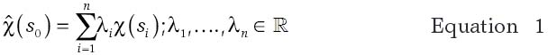
wher s₀; χ(s_i) corresponds to the curve observed at site s_i; and i = 1, 2,..., n and l_i, i = 1, ..., n, are the weighting parameters of each observed curve to the predicted curve. is the predicted curve at site

The l_i parameters are estimated by solving the following system of equations (Giraldo et al., 2010):

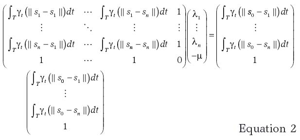
where the integrals are the trace-variogram function (Giraldo et al., 2010) evaluated for distances between the observation sites (matrix to the left of the equal sign) and the distances between the observation sites and the prediction site (vector to the right of the equal sign). These integrals are calculated by estimating the trace-variogram function, which is given by the following equation (Giraldo et al., 2010):

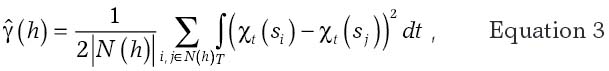
where corresponds to the number of sites (pairs) separated by distance and its subsequent fit with traditional parametric semivariance models (spherical, exponential, Gaussian, and Matérn).

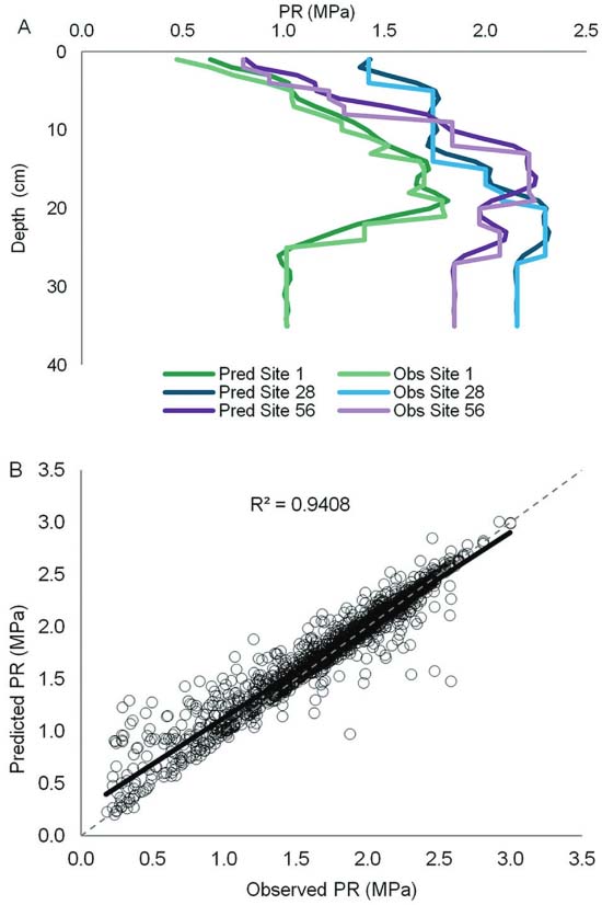
To calculate the prediction, the trace-semivariogram function was estimated using Equation 3. This function was later used in conjunction with Equation 2 to estimate l_i parameters for the functional Kriging predictor defined in Equation 1. The results of the estimation from Equation 3 and of the fit of a theoretical semivariance model to this function have not been included here for simplicity. To evaluate the goodness of fit of the functional Kriging predictor, three sites for which information was already obtained were selected randomly (sites 1, 28, and 56) and subjected to cross-validation. The curves for each site were removed from the dataset and subsequently predicted based on the functional Kriging predictor and the curves for the remaining 74 sites.

The results obtained from the functional Kriging predictor were compared with those obtained using univariate Kriging at depths of 1, 10, 20, and 30 cm (selected to compare predictions at surface, at intermediate depth, and at the lowest depths analyzed). To perform traditional analyses, the values for the PR values were determined at the depths mentioned above, and the semivariance function was calculated for each depth using the following equation (Cressie, 1993):

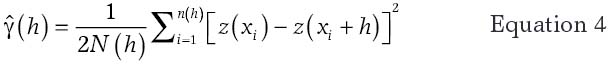
where z(x_i) is the PR value at point x_i; z(x_i+h) is the value of PR at a point with distance h from the previous point; and N(h) is the number of data pairs separated by distance h. Semivariance function is the model fitted to the experimental semivariogram. The following criteria were considered to select the best model: the coefficient of determination (R²), which indicate the ratio of change in the variable; the least sum of squared errors (LSSE) to predict the error between observed and estimated values from cross validation (CVC). The shared parameters among the theoretical semivariance models include the nugget (C₀), which is a discontinuity in the semivariogram at the origin, the variance of the process (C), and the range (r), which is the distance until a spatial correlation is obtained. The nugget-variance ratio [C/(C₀+C)] is often used as a criterion to select a model because it establishes the degree of spatial dependence (DSD) expressed by the studied attributes. Cambardella et al. (1994) suggested the following classifications for DSD: Strong, when DSD > 75 %; Moderate, when 25 % ≤ DSD ≤ 75 %; and Weak, when DSD < 25 %.

Results and Discussion

Descriptive analysis of soil penetration resistance

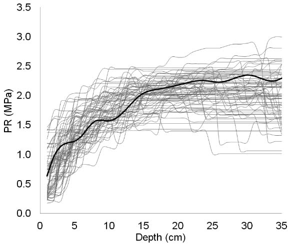
The soil examined for this study presents optimal root development at depths greater than 10 cm (Figure 1). While Bowen et al. (1994) identified critical values that ranges between 0.9 and 1.5 MPa for root growth, soils possessing a PR closer to 2.0 MPa were classified as having excessive compaction (Leao and Silva, 2006). Such compaction influences roots penetration through the soil (Chan et al., 2006; Hakansson and Lipiec, 2000; Hamza and Anderson, 2005), favors run-off and the accumulation of water on the surface due to a reduced number of porous spaces and the formation of a relatively impermeable surface layer (Islam et al., 2011; Gómez-Rodríguez et al., 2013).

Figure 1
– Mean soil penetration resistance (PR) curve for the studied location and confidence interval (points).

Descriptive statistics for PR in the studied region (for depths of 1, 10, 20, and 30 cm) are shown in Table 1. The means and medians were similar at each depth, and the skewness and kurtosis coefficients were close to zero. These results showed that the frequency distributions were symmetrical and presumably stationary (in terms of the mean) in the underlying stochastic process. Thus, we concluded that the mean PR fluctuates, and no clear trend can be found in the mean PR in this zone (at a particular depth). The increase of depth resulted in a significant increase in PR (Figure 1).

Table 1
– Statistical summary of soil penetration resistance (PR) obtained at 75 locations within a 37-ha plot in Puerto López, Meta, Colombia.

Depth (cm)	Mean	Median	CV (%)	Maximum	Minimum	Skewness	Kurtosis
1	0.64	0.62	55.9	1.47	0.18	0.72	-0.44
10	1.77	1.74	15.7	2.47	1.12	0.26	-0.06
20	2.08	2.10	12.0	2.65	1.40	-0.50	0.30
30	2.04	2.09	17.7	2.89	1.02	-0.49	0.75

• CV: Coefficient of variation; PR values at each location were recorded every millimeter from depths 0-35 cm. The results are only shown for four depths.

It is common in soil science studies that associate skewness coefficient values different from zero with non-normality. However, in spatial statistics, it is assumed that data are originated from a random process (stationary or non-stationary) and not from a particular variable. Then, when the random process is normal, the data are a realization (observation) of a multivariate normal distribution and not from an univariate normal distribution. Consequently, in spatial statistics, the skewness coefficient should not be used as an indicator of normality. However, from a descriptive point of view this coefficient can be considered to check empirically if the mean of the process is changing in the region. In spatial statistics, a skewness coefficient close to zero can be used as an indicator that the process is stationary, which means that average is not changing in the study area.

The relatively low coefficient of variation (CV) values at depths of 10, 20, and 30 cm (less than 20 %) (Table 1) indicated that the PR data presented low dispersion within locations. At a depth of 1 cm, the CV was 56 %. The increased variability in PR at 1 cm could be a consequence of human activities, mainly farming and cultural processes, and weathering processes, which are strongly linked to areas with high precipitation events.

Functional geostatistics analysis

The results described above only provide measures for a small selection of depths. Although these results undoubtedly allowed to establish general trends in the way PR behaves, they did not show the detailed way in which PR fluctuates at depth. A more complete picture of the behavior pattern exhibited by PR as a function of depth is shown in Figure 2 as raw data (A) and as smoothed data using B-spline basis (B). From a descriptive point of view, we concluded that the curves had less PR variability at shallower depths. Near the origin, PR varied between approximately 0 and 1.5 MPa, and at depths greater than 20 cm, where slopes of the curves approach zero, PR varied between 1.0 and 3.0 MPa. Figure 2 also shows a number of atypical PR curves (separated from the rest) at depths greater than 15 cm. These results would not be detectable using the data shown in Table 1.

Figure 2
− Soil penetration resistance (PR) recorded at 75 sites from a dedicated ranching area in Puerto López in Meta, Colombia (the curves shown are interpolated) (A) and smoothed curves result from the use of B-splines (B). Black lines is the mean PR values.

As an initial example of the application of this methodology, a predicted curve is shown in Figure 3 for the PR data obtained at the site with coordinates 952075 (W) and 1141025 (N) (4°09’52.8” N and 72°48’39.2” W). The predicted curve was similar to the behavior pattern of the observed data, which suggested that the soil does not present limitations for crop root growth for this zone (Carrara et al., 2007; Utset and Cid, 2003). At depths greater than 15 cm, compaction levels were greater than 2 MPa PR, which is the critical limit for root growth (Chan et al., 2006; Hakansson and Lipiec, 2000; Hamza and Anderson, 2005).

Figure 3
– Soil penetration resistance (PR) curves obtained by B-spline smoothing on data collected every millimeter in a zone from Puerto López, in Meta, Colombia (gray curves) and prediction of the PR curve using the Kriging functional predictor (black curve).

The original curves for randomly selected sites (1, 28 and 56) and their predicted equivalents are shown in Figure 4A. Each case showed evidence of goodness-of-fit, with similar predicted and smoothed observed curves. To obtain a numeric indicator of the goodness-of-fit, a simple linear regression was used to compare the 350 recorded values at each site with the 350 predicted values (Figure 4B). The observations and predictions were significantly correlated with a determination coefficient of 94 % (p < 0.001), which indicated that over 90 % of variability in the observed PR, data can be explained by the proposed predictor. In addition, the prediction worked best for PR values greater than 1.0 MPa due to the high variability of PR curves at shallow depths. Figure 4A shows that predictions resulting from functional geostatistical analysis had a good performance. Thus, this methodology allowed for a general characterization of the PR behavior at each prediction site to be obtained, which is an advantage over other classical statistical approaches that would provide only point-wise predictions. The use of traditional geostatistics with this type of data could be limited because it requires more computational time in addition to the modeling of many semivariograms (one for each depth).

Figure 4
− Superposition of the observed and predicted soil penetration resistance (PR) curves (A) and functional cross-validation of observed vs predicted PR values (B).

Validation of soil penetration resistance data

Using classical geostatistics, several authors have fitted semivariogram models to the PR data by considering exponential models (Barik et al., 2014; Veronese Junior et al., 2006). Medina et al. (2012) found that spherical PR models fit best at depths 1 and 20 cm and that exponential models fit best at depths 10 and 30 cm. Univariate geostatistical analysis of our data indicated that exponential models fit the data best at depths 1 and 30 cm and that spherical models fit best at depths 10 and 20 cm (Table 2). The more common semivariogram models for PR in geostatistical studies are the spherical an exponential models. However, these semivariogram models have been considered a good method to identify the structure of spatial variability for different physical properties in agricultural soils (Millán et al., 2012; Medina et al., 2012; Camacho-Tamayo et al., 20013; Barik et al., 2014).

Table 2
– Parameters of the semivariogram models fitted to observed (Obs) and predicted (Pre) penetration resistance (PR) data at four different soil depths (1, 10, 20 and 30 cm).

PR Depth	Model	C0	C0 + C	Range (m)	CVC	DSD
PR1Obs	Exponential	0.025	0.331	143.70	0.80	0.92
PR1Pre	Exponential	0.014	0.266	130.80	0.78	0.95
PR10 Obs	Spherical	0.002	0.025	151.00	0.69	0.94
PR10 Pre	Spherical	0.002	0.024	138.70	0.63	0.92
PR20 Obs	Spherical	0.000	0.011	110.50	0.73	1.00
PR20 Pre	Spherical	0.000	0.012	128.10	0.67	1.00
PR30 Obs	Exponential	0.003	0.031	158.40	0.60	0.89
PR30 Pre	Exponential	0.000	0.021	99.60	0.60	1.00

• Co: Nugget; Co+C: Sill; CVC: coefficient of cross validation; DSD: degree of spatial dependence.

Generally, C₀ values near zero at each analyzed depth and a degree of spatial dependence greater than 75 % indicate a strong spatial dependence (Cambardella et al., 1994). To compare the results graphically obtained by functional geostatistics with those obtained by classical geostatistics, spatial distribution maps were built with both methodologies at depths 1, 10, 20, and 30 cm (Figure 5). These maps indicated that the methodologies led to different results, and this difference was particularly evident at the 1 and 10 cm depths. Surfaces on the right, obtained with the predictions by functional Kriging (Figure 5), were more smoothed than surfaces on the left, which were obtained by classical Kriging, which is associated to the effect of data smoothing caused by the use of B-splines, as a previous step for the functional geostatistical analysis. This procedure allowed eliminating the data noise before performing the prediction step. Goodness-of-fit was evident based on the visible and irregular decrease or increase of PR in a number of zones, which is a behavior observed in both plots drawn from recorded and predicted data.

Figure 5
− Spatial distribution of penetration resistance (PR) obtained with classical geostatistics (left) and by using functional geostatistics (right) at soil depths 1, 10, 20, and 30 cm.

As a final step in evaluating functional prediction techniques, simple linear regressions were calculated to compare the 75 observed PR values with the 75 PR predictions obtained at each depth 1, 10, 20 and 30 cm after using functional geostatistics (Figure 6). High correlations were found between the observations and predictions, and coefficients of determination increased with increasing soil depth.

Figure 6
− Relationship between observed and predicted penetration resistance (PR) at soil depths 1, 10, 20, and 30 cm.

Conclusions

Functional data with spatial dependence allows techniques from spatial statistics and functional data analysis to be combined. This study showed how this kind of approach can be used to model PR data. Our results indicated that this alternative proved to be useful.

Creating spatial distribution maps for the observed and predicted PR values allowed the differences between recording sites to be clearly visualized as well as the similar behaviors between the observed and predicted data. In addition, better fits and greater homogeneity were found at greater depths.

Even considering that ordinary Kriging for functional data is a good approach, other alternatives, such as continuous time varying Kriging for functional data or a functional Kriging total model, could be considered and compared in future studies.

References

• Barik, K.; Aksakal, E.L.; Islam, K.R.; Sari, S.; Angin, I. 2014. Spatial variability in soil compaction properties associated with field traffic operations. Catena 120: 122-133.
• Bowen, H.D.; Garner, T.H.; Vaughn, D.H. 1994. Advances in soil-plant dynamics. In: ASAE. Advances in soil dynamics. ASAE, St. Joseph, MI, USA.
• Caballero, W.; Giraldo, R.; Mateu, J. 2013. A universal kriging approach for spatial functional data. Stochastic Environmental Research and Risk Assessment 27: 1553-1563.
• Camacho-Tamayo, J.H.; Rubiano Sanabria, Y.; Santana, L.M. 2013. Management units based on the physical properties of an Oxisol. Journal of Soil Science and Plant Nutrition 13: 767-785.
• Cambardella, C.A.; Moormam, T.B.; Novak, J.M.; Parkin, T.B.; Karlen, D.L.; Turco, R.F.; Konopka, A.E. 1994. Field-scale variability of soil properties in central Iowa soils. Soil Science Society of America Journal 58: 1501-1511.
• Carrara, M.; Castrignanò, A.; Comparetti, A.; Febo, P.; Orlando, S. 2007. Mapping of penetrometer resistance in relation to tractor traffic using multivariate geostatistics. Geoderma 142: 294-307.
• Chan, K.; Oates, A.; Swan, A.; Hayes, R.; Dear, B.; Peoples, M. 2006. Agronomic consequences of tractor wheel compaction on a clay soil. Soil and Tillage Research 89: 13-21.
• Cressie, N. 1993. Statistics for Spatial Data. John Wiley, New York, NY, USA.
• Giraldo, R.; Delicado, P.; Mateu, J. 2010. Continuous time-varying Kriging for spatial prediction of funtional data: an environmental application. Journal of Agricultural, Biological, and Environmental Statistics 15: 66-82.
• Gómez-Rodríguez, K.; Camacho-Tamayo, J.H.; Vélez-Sánchez, J.E. 2013. Changes in water availability in the soil due to tractor traffic. Engenharia Agrícola 33: 1156-1164.
• Guimarães, R.M.L.; Ball, B.C.; Tormena, C.A.; Giarola, N.F.B.; Silva, A.P. 2013. Relating visual evaluation of soil structure to other physical properties in soils of contrasting texture and management. Soil and Tillage Research 127: 92-99.
• Hakansson, I.; Lipiec, J. 2000. A review of the usefulness of relative bulk density values in studies of soil structure and compaction. Soil and Tillage Research 53: 71-85.
• Hamza, M.; Anderson, W. 2005. Soil compaction in cropping systems: a review of the nature, causes and possible solutions. Soil and Tillage Research 82: 121-145.
• Hoef, J.; Cressie, N. 1993. Multivariable spatial prediction. Mathematical Geology 25: 219-240
• Islam, M.M.; Saey, T.; Meerschman, E.; Smedt, P.; Meeuws, F.; Vijver, E.; Meirvenne, M. 2011. Delineating water management zones in a paddy rice field using a floating soil sensing system. Agricultural Water Management 102: 8-12.
• Leao, T.P.; Silva, A.P. 2006. A statistical basis for selecting parameters for the evaluation of soil penetration resistance. Scientia Agricola 63: 552-557.
• Medina, C.; Camacho-Tamayo, J.H.; Cortes, C. 2012. Soil penetration resistance analysis by multivariate and geostatistical methods. Revista Brasileira de Engenharia Agrícola e Ambiental 32: 91-101
• Millán, H.; Tarquís, A.M.; Pérez, L.D.; Mato, J.; González-Posada. M. 2012. Spatial variability patterns of some Vertisol properties at a field scale using standardized data. Soil and Tillage Research 120: 76-84.
• Myers, D. 1982. Matrix formulation of co-kriging. Mathematical Geology 14: 249-257
• Orjuela-Matta, H.M.; Rubiano, Y.; Camacho-Tamayo, J.H. 2012. Spatial analysis of infiltration in an oxisol of the eastern plains of Colombia. Chilean Journal of Agricultural Research 72: 404-410.
• Ramsay, J.; Silverman, B. 2005. Functional Data Analysis 2. Springer, New York, NY, USA.
• Reyes, A.; Giraldo, R.; Mateu, J. 2015. Residual kriging for functional spatial prediction of salinity curves. Communications in Statistics - Theory and Methods 44: 798-809.
• Utset, A.; Cid, G. 2003. Soil penetrometer resistance spatial variability in a Ferralsol at several soil moisture conditions. Soil and Tillage Research 61: 193-202.
• Veronese Júnior, V.; Carvalho, M.P.; Dafonte, J.; Freddi, O.S.; Vidal Vázquez, E.; Ingaramo, O.E. 2006. Spatial variability of soil water content and mechanical resistance of Brazilian ferralsol. Soil and Tillage Research 85: 166-177.

Edited by

Edited by: Paulo Cesar Sentelhas

Publication Dates

• Publication in this collection
  Sep-Oct 2016

History

• Received
  24 Mar 2015
• Accepted
  18 Dec 2015