Bayesian sequential procedure to estimate the viability of seeds Coffea arabica L. in tetrazolium test

ABSTRACT:

Tetrazolium tests use conventional sampling techniques in which a sample has a fixed size. These tests may be improved by sequential sampling, which does not work with fixed-size samples. When data obtained from an experiment are analyzed sequentially the analysis can be terminated when a particular decision has been made, and thus, there is no need to pre-establish the number of seeds to assess. Bayesian statistics can also help, if we have sufficient knowledge about coffee production in the area to construct a prior distribution. Therefore, we used the Bayesian sequential approach to estimate the percentage of viable coffee seeds submitted to tetrazolium testing, and we incorporated priors with information from other analyses of crops from previous years. We used the Beta prior distribution and, using data obtained from sample lots of Coffea arabica, determined its hyperparameters with a histogram and O’Hagan's methods. To estimate the lowest risk, we computed the Bayes risks, which provided us with a basis for deciding whether or not we should continue the sampling process. The results confirm that the Bayesian sequential estimation can indeed be used for the tetrazolium test: the average percentage of viability obtained with the conventional frequentist method was 88 %, whereas that obtained with the Bayesian method with both priors was 89 %. However, the Bayesian method required, on average, only 89 samples to reach this value while the traditional estimation method needed as many as 200 samples.

Keywords:
Beta distribution; seed analysis; sampling; coffee; prior distribution

Introduction

The tetrazolium test is a method for quickly assessing seed viability and vigor (Clemente et al., 2011; Rosa et al., 2010). A sample for the test must be collected according to the guide provided by the International Seed Testing Association (ISTA, 2008). Widely used in agricultural research, these sampling rules originated in quality control techniques. However, because of the expediency of the planting time, seeds need fast decisions so that they can be released for cultivation or commercialization.

Conventional sampling methods are based on a fixed number of sampling units. Sequential sampling is a faster, reliable and more efficient alternative to the fixed-sample-size method (Mukhopadhyay and Silva, 2009). In sequential sampling, the number of sample units varies, which can help reduce sampling time with no loss of reliability. Further, the sampling units are tested in sequence until the data gathered is sufficient for estimating the parameters and can be subjected to testing hypotheses (Zacks, 2017; Souza et al., 2014).

Among the various applications of sequential sampling, we highlight the articles of Souza et al. (2014) and Ballaris et al. (2014) who used sequential sampling to determine the number of seeds required to accurately verify lot infestation.

Sequential sampling may be improved by using what we know about coffee production in the area: for example, we might have garnered useful indications from analyses of crops from previous years, or information about the genotype of the seeds assessed. Such knowledge can allow the use of Bayesian inference for sequential sampling.

Bayesian statistics draws on previous research knowledge to analyze the present data (Morita et al., 2008). Several techniques are available for the building of a probabilistic prior distribution for the viability of a lot of seeds. The usual technique consists of deciding on a possible distribution based on a histogram of the variable. Another builds on the prior density function based on probabilistic specifications provided, for example, by an expert. Such knowledge can be translated into percentages of a probability distribution by elicitation (Garthwaite et al., 2005).

Since Bayesian statistics uses prior knowledge, it can be more precise than traditional frequentist statistics. This enhanced precision, may require fewer seeds when applied to the tetrazolium test. Thus, we used the Bayesian sequential approach to estimate the percentage of viable coffee seeds submitted to the tetrazolium test, incorporating priors with information from experiments on crops from previous years. Next, we compared the results with those of the traditional frequentist approach applied to the tetrazolium test. Although our method focused on coffee seeds, it can also be applied to seeds of other species that are analyzed in a similar way.

Materials and Methods

Evaluation of the percentage of viable coffee seeds submitted to the tetrazolium test

We conducted the tetrazolium test in 25 lots of Coffea arabica, coming from the 2015/2016 crop in the area of Lavras (latitude 21°30’ S, longitude 44°60’ W and average elevation of 919 m), south Minas Gerais, Brazil, to assess their viability.

The sample seeds were collected in accordance with Normative Instruction no. 9 of the Ministry of Agriculture, Livestock and Supply, June 2, 2005, which approves rules for the production, commercialization and use of seeds in Brazil (MAPA, 2009; Santos et al., 2014).

To validate the procedure proposed in this work, we ran the conventional tetrazolium test for 200 coffee seeds (AOSA, 1983), divided into two repetitions with 100 seeds in each lot. Seeds are soaked in distilled water for 48 hours, the embryos were extracted and kept in an antioxidant solution of polyvinylpyrrolidone (PVP) until they were placed in the tetrazolium solution. At the end of the extraction, the embryos were washed in running water then sieved and imbibed in 0.5 % tetrazolium solution, in darkness (using dark flasks), at a temperature of 30 °C, for 2 hours.

We analyzed viability with a stereoscopic magnifying glass: based on the location and extension of the areas stained by the tetrazolium salt, we rated the embryos as viable or not viable.

According to the International Seed Analysis Association, results of a viability test should only be accepted if the difference between the repetitions with the highest and the lowest estimated viability percentage does not exceed the tolerance level (Bányai and Barabás, 2002).

To check the test reliability, we estimated the mean percentage viability for the repetitions, which was compared with the tolerance value (table value) at a significance level of 5 % (Miles, 1963).

Construction of the prior distribution using information from previous experiments

The tetrazolium test gives results that resemble a Bernoulli trial, since each rated seed may be characterized as either viable or not viable. Thus, each result has associated probabilities of success (viable) (p) and failure (not viable) (1–p). In accordance with this specification, x corresponds to the sum of successful Bernoulli trials, that is, the total number of viable seeds in an n-sized sample, and is defined by the binomial distribution X ∼ Bin(n,p)

(1) $$f\left(x|p\right)=\left(\begin{array}{c}n\\ x\end{array}\right)p^x{\left(1-p\right)}^{n-x}0\le p\le 1$$

where p is the population proportion (or percentage) of viable seeds in a lot, and n the sample size. The formula (1) represents the probability of drawing a sample of n seeds of which x are viable. According to Bányai and Barabás (2002), germination data follow the binomial distribution.

In the Bayesian context, the proportion p of viable seeds is considered random variable P, to which a prior probability distribution π(p) is associated. From the experimental information provided by the likelihood function f(x|p), we obtain a posterior distribution f(p|x) (Pham-Gia, 1998). Consequently, the posterior distribution f(p|x) for parameter p will be f(p|x) ∝ f(x|p).π (x). When a prior distribution is defined in the class of conjugated distributions, it is possible to obtain a posterior distribution which has the same functional form as these likelihood functions (Berger, 1985). The use of conjugate priors is just a convenient mathematical device.

According to Gelman (2006), the Beta conjugated prior distribution P ∼ Beta(α,β) is often used to model random variables representing proportions and percentages. This distribution has the following form:

(2) $$\text{π}\left(p|\mathrm{\alpha },\mathrm{\beta }\right)=\frac{\mathrm{\Gamma }\left(\mathrm{\alpha }+\mathrm{\beta }\right)}{\mathrm{\Gamma }\left(\mathrm{\alpha }\right)\mathrm{\Gamma }\left(\mathrm{\beta }\right)}{p}^{\mathrm{\alpha }-1}{\left(1-p\right)}^{\mathrm{\beta }-1}$$

where 0 ≤ p ≤ 1, $\mathrm{\Gamma }\left(\mathrm{\alpha }\right)={\displaystyle {\int }_0^{\infty }{u}^{\mathrm{\alpha }-1}{e}^{-u}du}$ is the Gama function, and the hyperparameters are α > 0 and β > 0. In Bayesian statistics, a hyperparameter is the parameter of a prior distribution; the term is used to distinguish hyperparameters from parameters of the analyzed model. In this work p is a parameter of the Binomial distribution while α and β are parameters of the prior distribution (Beta distribution), thus, hyperparameters.

With changing hyperparameters, the Beta distribution shape can change, too. When α > 1 and β > 1, the distribution is unimodal and skewed with its single mode at

$$p=\frac{\left(\mathrm{\alpha }-\text{1}\right)}{\left(\mathrm{\alpha }+\mathrm{\beta }-2\right)};$$

this mode would be the most frequent proportion of viable seeds in a lot. The expected proportion E(p), the proportion's variability Var(p) and the mode corresponding to the most likely value are, respectively,

(3) $$\begin{array}{l}E\left(p\right)={\text{μ}}_{priori}=\frac{\mathrm{\alpha }}{\left(\mathrm{\alpha }+\mathrm{\beta }\right)},\\ Var\left(p\right)={\text{σ}}^2{}_{priori}=\frac{\left(\text{αβ}\right)}{{\left(\mathrm{\alpha }+\mathrm{\beta }\right)}^2\left(\text{α+β+1}\right)}\text{and}\\ \text{mode}=\frac{\mathrm{\alpha }-1}{\left(\mathrm{\alpha }+\mathrm{\beta }-2\right)},\end{array}$$

We can use several approaches to determine hyperparameters α and β from the prior distribution (2) (Paulino et al., 2005). To create a prior distribution, we tried the histogram method and then O’Hagan's elicitation method.

We constructed the first prior Beta distribution (α_hist, β_hist) based on the histogram derived from historical data obtained by the expert in a traditional tetrazolium test carried out in 2015 with 17 lots of Coffea arabica L., in Lavras, Minas Gerais, Brazil. The histogram was built by partitioning the parametric space [0;1] into sub-intervals of length where h = 0.2. Afterwards, we calculated from the historical data the probability for each sub-interval to contain the true parametric value, and built the histogram. We then adjusted the Beta distribution to this histogram by using our R script (R Core Team, 2015) and found mean $\widehat{\text{μ}}$ and variance ${\widehat{\text{σ}}}^{\text{2}}$ of this distribution.

Applying the moment method, we estimated α and β as

(4) $${\widehat{\mathrm{\alpha }}}_{hist}=\widehat{\text{μ}}\left(\frac{\widehat{\text{μ}}\left(1-\widehat{\text{μ}}\right)}{{\left({\widehat{\text{σ}}}^{\text{2}}\right)}^2}-1\right)\text{and}{\widehat{\mathrm{\beta }}}_{hist}=\left(1-\widehat{\text{μ}}\right)\left(\frac{\widehat{\text{μ}}\left(1-\widehat{\text{μ}}\right)}{{\left({\widehat{\text{σ}}}^{\text{2}}\right)}^{\text{2}}}-1\right)$$

It is impracticable to expect experts unfamiliar with Bayesian statistics to understand how hyperparameters work in a probability distribution. Thus, we used an adaptation of the elicitation method proposed by O’Hagan (1998), with which we helped the expert to elicit all the information obtained from the analyses based on crops from previous years. Choosing a candidate distribution for the prior distribution is important, especially when there is not much information about the shape of the target density and, in this case, the parametric space or the domain of a function for p is the interval [0;1] (Cappé et al., 2008). First, we elicited the mode (m), the Lower limit (L) and the Upper Limit (U) of the candidate distribution to model the parameter p. Afterwards, we calculated probabilities prob_i associated with six different intervals of occurrence of viability of parameter p (Moala and Penha, 2016):

(5) $$\begin{array}{l}pro{b}_1=\text{Probability}\left(L<p<m\right);\\ pro{b}_2=\text{Probability}\left(L<p<\frac{L+m}{2}\right);\\ pro{b}_3=\text{Probability}\left(\frac{U+m}{2}<p<U\right)\\ pro{b}_4=\text{Probability}\left(L<p<\frac{L+3m}{4}\right);\\ pro{b}_5=\text{Probability}\left(\frac{U+3m}{4}<p<U\right).\end{array}$$

Afterwards, we converted probabilities prob_i into six quantiles as follows: $q_1=p_2$; $q_2=p_4-p_2$; $q_3=p_1-p_4$; $q_4=1-p_1-p_5$; $q_5=p_5-p_3$; and $q_6=p_3$.

Thus, we used several values of α and β to establish the Beta distribution $Beta\left({\widehat{\mathrm{\alpha }}}_{OHagan},{\widehat{\mathrm{\beta }}}_{OHagan}\right)$ that best represents expert opinion about historical data; in so doing, we developed an algorithm (see the code in ^Appendix) to find hyperparameters $\left(\widehat{\mathrm{\alpha }},\widehat{\mathrm{\beta }}\right)$ to minimize the sum of squares of the differences between the elicited probabilities and the probabilities of another Beta distribution, Beta(α, β)(Garthwaite et al., 2005). We considered the intervals α ∈ [1;30] and β ∈ [1;30] We chose these intervals because when α >1 and β >1, the distribution is unimodal and skewed with a single mode. Furthermore, the distribution is strongly right-skewed when β is much greater than α, but the distribution gets less skewed and the mode approaches 0.5 as α and β approach each other (Lau and Lau, 1991). For this reason, estimates of mean, median and mode can be different. The limit equal to 30 allows for all the possibilities to have occurred.

Stopping Rule and Estimation Criteria for the Bayesian Sequential Procedure

At each step of the sequential inspection, we calculated the values of loss function L(p, δ_n, n), where p is the proportion of viable seeds, δ_n a decision function and n, the sample size up to that moment. A loss function L is the loss incurred by adopting decision δ_n when the true state of nature is p (Brockwell and Kadane, 2003) One of the most used loss functions in decision theory is the quadratic loss function $L={\left(p-\widehat{p}\right)}^2$, where p is the viability proportion expected for a lot of seeds while $\widehat{p}$ is the actual proportion in the sample.

Based on sequential decision theory, we treated the cost as constant, but it could also be linear or even a quadratic function. Pham-Gia (1998) considered the quadratic loss function plus a sampling cost of one unit (here, one seed) per observation:

(6) $$L=\left(p,d_n,n\right)={\left(p-\widehat{p}\right)}^2+C\left(n\right)$$

where C(n) > 0 is the cost function to use an n-size sample to estimate proportion p.

We treated the cost as a constant, so we did not estimate it. Thus, we did not update it during the estimation process; instead, we multiplied the cost value by the size of the sample.

The risk function of a sequential procedure is the expected loss, $R\left(p\right)=E\left[L\left(p,{\text{δ}}_n,n\right)\right]=E\left[{\left(p-\widehat{p}\right)}^2+C\left(n\right)\right]$. Our aim was to develop such an inspection plan that minimizes the risk function. Brockwell and Kadane (2003) report that ‘the Bayesian approach to sequential analysis is to select a procedure that stops the sampling, allowing to minimize the expected value of some loss function which reflects the cost associated with a particular outcome’. However, the value attributed to the cost must have an order of magnitude similar to the order of magnitude of ${\left(p-\widehat{p}\right)}^2$, which ensures that the risk function is not exclusively dominated by cost. Since the loss is the square of a difference between the proportion values which are between 0 and 1 the results are always close to zero and the cost should be close to zero, too (Bach, 2015). Consequently, the cost is a factor of minor impotance to making a decision of when to interrupt sampling.

Brockwell and Kadane (2003) report that ‘the Bayesian approach to sequential analysis is select a procedure that stops the sampling allowing minimizing of the expected value of some loss function which reflects the perceived cost associated with a particular outcome’. In the Bayesian sequential procedure, we must also calculate the Bayes risk, defined by r(π) = E^π [R(p)], that is, the expected risk associated with the estimation procedure of parameter p, given prior π after n observations (Berger, 1985).

Pratt et al. (1964) demonstrated that the posterior Bayes risk is the variance of the posterior distribution where:

(7) $$r_o\left({\text{π}}^n,n\right)=va{r}_{post}\left(n\right)$$

Thus, the expected posterior Bayes risk when another observation is made is (Pham-Gia, 1998):

(8) $$r^1\left({\text{π}}^n,n\right)=E\left[va{r}_{post}\left(n\right)\right]$$

A risk function governs the stopping rule. The general idea in Bayesian sequential analysis is that it is necessary to calculate the immediate risk r_o(πⁿ, n) after each seed has been observed and make a comparison with the expected posterior Bayes risk r¹(πⁿ, n), that is, the risk for a situation where one more seed is observed (Berger, 1985).

The standard procedure after evaluating the n^th seed is to compare r_o(πⁿ, n) with r¹(πⁿ, n). If r_o(πⁿ, n) > r¹(πⁿ, n), the sampling continues; if r_o(πⁿ, n) ≤ r¹(πⁿ, n), the sampling stops. Bayes Sequential Rule may also be known as Bayesian learning, because the posterior distribution calculated at current n will be used to update the prior distribution yet to be used at the (n+1)^th inspection (Garthwaite et al., 1995).

Since we used the squared-error loss, the mean of the posterior distribution was Bayes’ estimator of proportion p. Thus, we estimated the proportion of viable seeds in the lot using the Beta (α’, β’) distribution (Berger, 1985) mean.

The expected value µ_post and variance ${\text{σ}}_{post}^2$ of the posterior distribution of p are given by the Beta distribution with parameters as follows:

(9) $$\begin{array}{l}{\text{μ}}_{post}=\frac{\mathrm{\alpha }+x}{\left(\mathrm{\alpha }+x+\mathrm{\beta }+n-x\right)}\text{and}\\ {\text{σ}}_{post}^2=\frac{\left(\mathrm{\alpha }+x\right)\left(\mathrm{\beta }+n-x\right)}{{\left(\mathrm{\alpha }+\mathrm{\beta }+n\right)}^2\left(\mathrm{\alpha }+\mathrm{\beta }+n+1\right)}.\end{array}$$

Consequently, the expectancy of variance $E[va{r}_{post}(n)]$ is $\left(\frac{\mathrm{\alpha }+\mathrm{\beta }+n}{\mathrm{\alpha }+\mathrm{\beta }+n+\text{1}}\right){\mathrm{var}}_{post}$

Thus, according to (7), (8) and (9), the stopping criterion will be

(10) $$\begin{array}{l}\frac{\left(\mathrm{\alpha }+x\right)\left(\mathrm{\beta }+n-x\right)}{{\left(\mathrm{\alpha }+\mathrm{\beta }+n\right)}^2\left(\mathrm{\alpha }+\mathrm{\beta }+n+1\right)}\le \\ \left(\frac{\mathrm{\alpha }+\mathrm{\beta }+n}{\mathrm{\alpha }+\mathrm{\beta }+n+1}\right)\frac{\left(\mathrm{\alpha }+x\right)\left(\mathrm{\beta }+n-x\right)}{{\left(\mathrm{\alpha }+\mathrm{\beta }+n\right)}^2\left(\mathrm{\alpha }+\mathrm{\beta }+n+1\right)}.\end{array}$$

Therefore, according to (6) and (10):

(11) $$r_0\left({\text{π}}^n,n\right)+\left(n\right)c\le \left(\frac{\mathrm{\alpha }+\mathrm{\beta }+n}{\mathrm{\alpha }+\mathrm{\beta }+n+1}\right)r_0\left({\text{π}}^n,n\right)+\left(n+1\right)c.$$

Here, (n)c and (n+1)c are the costs of observing n and n+1 sample units.

We implemented the above procedure in R. The process to build each prior is carried out only once. On the other hand, the sequential procedure is performed for each lot, that is, we did it 25 times (see the code in ^Appendix).

Results and Discussion

Construction of prior distributions

According to the above-described procedures, we obtained a histogram from the percentages of seed viability in 17 coffee lots from the analysis carried out for crops harvested in 2015; when calculating the hyperparameters according to equation (4), we found that the best distribution was Beta with hyperparameters α = 9.14 and β = 1.29 (Table 1).

Table 1
Estimations of hyperparameters considering the different methods to build priors.

Bayesian Sequential Procedure	Beta prior		Measures
	α	β	Mode	Average	Standard deviation
			------------------ % --------------------
Histogram	9.14	1.29	96.56	87.63	0.0975
O’Hagan	27.20	2.70	93.91	90.97	0.0520

To build the prior by O’Hagan's method, we calculated the sum of squares of the differences between the probabilities elicited from historical data and the probabilities in different Beta distributions, according to the quantiles considered in expression (5). We considered the inspection of values α; β for intervals α ∈ [1;30] and β ∈ [1;30] with a gap of length 0.1. We selected the pair of hyperparameters, α = 27.2 and β = 2.7, which provided the lowest sum of squares of the differences (Moala and Penha, 2016).

Implementing O’Hagan's method, we determined the pair of values of (α; β) that minimize the sum of squares of the differences between probabilities elicited by the historical information and the probabilities of Beta distribution (α; β) (Moala and Penha, 2016). The smallest sum of squares for α was 27.2 and for β, 2.7 (Table 1).

The prior histogram method led to a lower mean percentage of viable seeds with greater variability, whereas the prior obtained by the adapted O’Hagan's method resulted in a higher but more precise mean. Figure 1 visualizes the prior probability functions. They indicate that the histogram method presented heavier tails; therefore, for smaller proportions, there is evidence that the probabilities estimated by this method will be higher.

Figure 1
Comparison of prior densities.

For the mode measure, the histogram method is equivalent to O’Hagan's, so either method may be used. Moala and Penha (2016) mention other studies which show that, when the sample distribution is slightly asymmetric, the estimations of mode, mean and median may be imprecise. Hughes and Madden (2002) reviewed methods that may be used to adjust the Beta distribution to an expert's opinion.

Both Bayesian procedures were superior to the classic frequentist approach. The difference between sample sizes in the Bayesian procedures was close to two units, which may be considered insignificant.

Estimation of the percentage of viable coffee seeds in the tetrazolium test using traditional sampling and Bayesian sequential procedure

To compare the Bayesian and traditional methods, we estimated the percentage of viable seeds in each of the 25 lots from the 2016 crop using the Bayesian approach for each prior built with the information gathered from the 2015 crop. From each procedure we defined the initial proportion, calculated by the mean posterior μ_post, and variance ${\text{σ}}_{post}^2$ given by (9). For each seed assessed, we assigned a dummy variable, with values coded as 1 and 0, which represent seed results as viable seeds (value 1) or inviable seeds (value 0), respectively. For each new seed, we obtained the hyperparameters of the posterior distribution (α’ and β’) and the corresponding risks. The decision as to whether to continue the sampling to stop was based on checking whether the expected risk r¹ was greater than the immediate risk r_o.

The values calculated for Bayes risk differed only in the sixth decimal place. If the cost is too high, the procedure stops after analyzing a few seeds, thus, we opted for a fixed cost value (10⁻⁷) for each seed. This is a situation in which observations are cheap when compared to the decision loss (Berger, 1985). Therefore, fixed costs had a penalty, but this also ensured that the cost is not the only variable to affect the decision-making process.

For example, we considered 10⁻⁷ as the cost per observation where α_hist=9.14 and β_hist=1.29 were the hyperparameters of the first prior distribution. Adopting Bernoulli's process as a viable (x_i=1) or not viable (x_i=0) seed, we obtained the result below.

If the first seed is viable, then x₁ = 1, thus and (according to the Beta distribution parameters). The immediate risk (7) was

$$r_0\frac{\left(10.14+1\right)\left(1.29+1-1\right)}{{\left(10.14+1.29+1\right)}^2\left(10.14+1.29+1+1\right)}+\left(1\right)\left({10}^{-7}\right)=0.0069257$$

and the expected risk (8) was

$$r^1=\left(\left(1\right)\frac{10.14+1.29+1}{10.14+1.29+1+1}\right)\times 0.00692559+\left(2\right)\left({10}^{-7}\right)=\mathrm{0.0064101.}$$

Thus, since r₀ > r¹, we decided to continue the sampling, sequentially, until the sampling was interrupted when r₀ ≤ r¹. The resulting sample size (n), the percentage of viable seeds (p), the hyperparameters we used (α; β) and the posterior parameters (α’; β’) are described in Table 2.

Table 2
Percentage of viable coffee seeds obtained from the tetrazolium tests, using traditional sampling and Bayesian sequential sampling with different priors.

Seed Lots	Conventional n = 200	Sequential procedure
		Histogram Beta prior				O’Hagan's Beta prior
	%	%	n	α	β	%	n	α	β
1	89.5	86.82	98	94.14	14.29	87.86	83	98.69	13.64
2	89.5	87.51	96	93.14	13.29	87.86	83	98.69	13.64
3	90.0	91.40	86	88.14	8.29	95.73	56	81.69	3.64
4	91.0	91.40	86	88.14	8.29	92.39	71	92.69	7.64
5	91.5	95.75	67	74.14	3.29	94.86	61	85.69	4.64
6	74.0	73.87	117	94.14	33.29	77.43	102	26.69	2.64
7	85.0	93.88	76	81.14	5.29	93.18	68	90.69	6.64
8	92.0	93.88	76	81.14	5.29	93.96	64	87.69	5.64
9	93.5	95.75	67	74.14	3.29	94.86	61	85.69	4.64
10	92.5	93.88	76	81.14	5.29	93.18	68	90.69	6.64
11	91.0	88.23	94	92.14	12.29	87.86	83	98.69	13.64
12	95.5	93.88	76	81.14	5.29	93.18	68	90.69	6.64
13	91.0	88.97	92	91.14	11.29	88.65	82	98.69	12.64
14	84.5	87.51	96	93.14	13.29	89.35	80	97.69	11.64
15	94.0	93.04	80	84.14	6.29	92.39	71	92.69	7.64
16	89.0	89.75	90	90.14	10.29	90.09	78	96.69	10.64
17	71.0	76.65	115	96.14	29.29	80.50	97	101.69	24.64
18	78.5	80.50	109	96.14	23.29	84.51	91	101.69	18.64
19	85.5	85.38	101	95.14	16.29	86.56	87	100.69	15.64
20	93.0	89.75	90	90.14	10.29	90.09	78	96.69	10.64
21	83.5	83.29	105	96.14	19.29	87.20	85	99.69	14.64
22	79.5	87.51	96	93.14	13.29	87.20	85	99.69	14.64
23	88.5	89.75	90	90.14	10.29	90.09	78	96.69	10.64
24	93.5	97.93	52	61.14	1.29	96.67	50	76.69	2.64
25	90.5	88.23	94	92.14	12.29	88.65	82	98.69	12.64

The three different methods—the conventional one and the two Bayes sequential approaches—led to a similar percentage of viable seeds for the lots (Table 2).

The Bayesian sequential method has advantages over the traditional method. By treating the parameter p as random, the Bayesian inference stems quite naturally from probability theory. This has many advantages and means that all inferential issues can be addressed as probability statements about p, which derive directly from the posterior distribution obtained for each lot and offer more information on the percentage of the estimated viability of seeds. Thus, in addition to point estimation and estimates, Bayesian statistics offers interval estimators called credibility intervals. Credibility intervals are similar to confidence intervals in frequentist statistics.

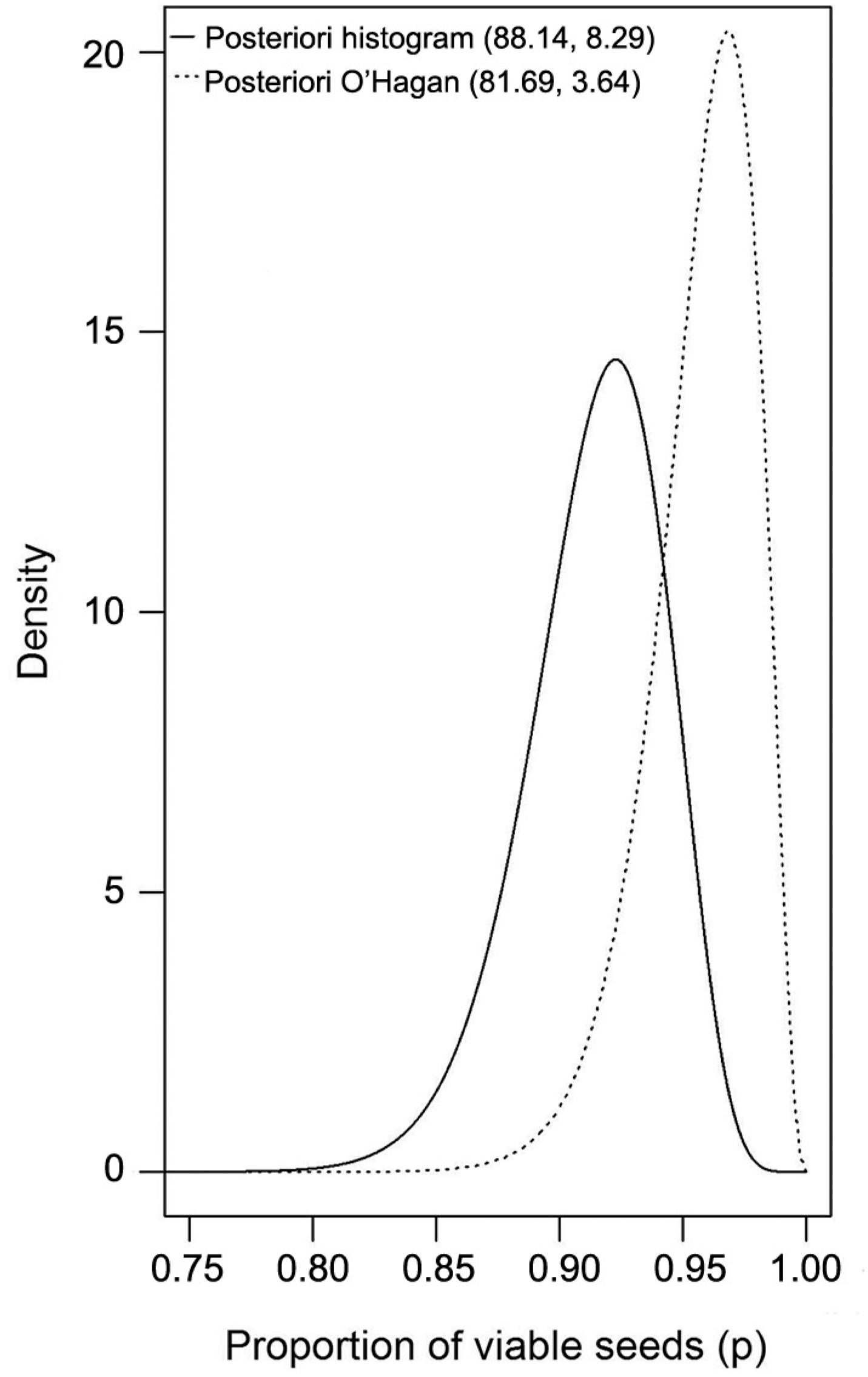
For a 95 % credibility level, the limits in the credibility range correspond to quantiles 0.025 and 0.975 of the posterior distribution for the distribution of interest. Figure 2 shows the graphical representation of the posterior distribution for one of the lots.

Figure 2
Posterior density for the percentage of viable coffee seeds in lot 3, obtained with the histogram and O’Hagan methods.

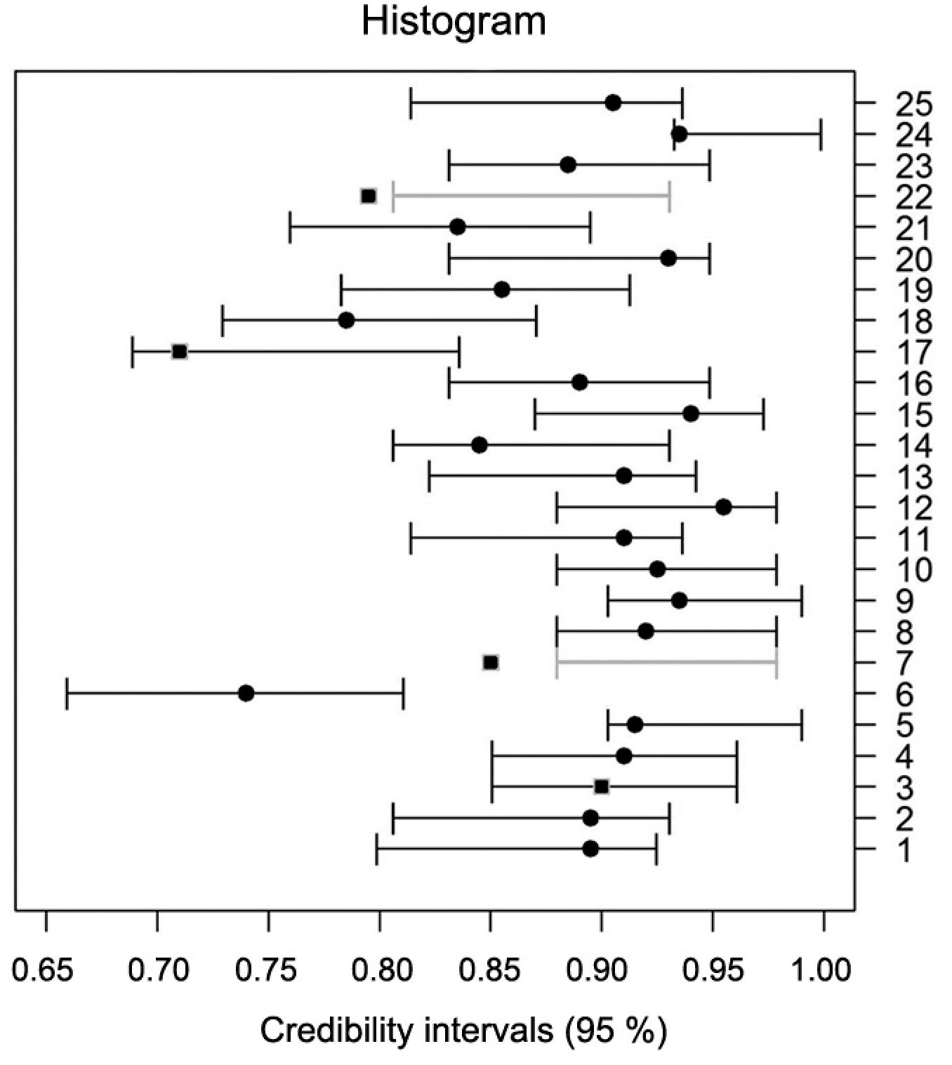
Compared to frequentist methods, Bayesian methods are especially helpful when the prior contributes a substantial share of the information (Van de Schoot et al., 2014; Agresti and Min, 2005; Bayarri, and Berger, 2004). We can compare the two methods by checking if the credibility intervals contained the frequentist estimate of p. For most lots they did, except for lots 7 and 22 by the histogram method (Figure 3) and for lots 3, 7, 17 and 22 by O’Hagan's prior method (Figure 4).

Figure 3
Credibility Intervals constructed by Histogram method and with the frequentist average (●).

Figure 4
Credibility Intervals constructed by O’Hagan method and with frequentist average (●).

Notice that in Figures 3 and 4 the credibility intervals constructed by both methods in each lot were nearly identical. For lots 7 and 22, the credibility intervals from both methods did not include the point estimate obtained by the frequentist method. For lots 3 and 17, the credibility interval constructed by the O’Hagan method did not include the frequentist point estimate perhaps because in O’Hagan's method, the prior was obtained from a smaller sample size. Consequently, it was less informative, that is, the error was more influenced by the data obtained.

According to the tolerance criteria, considering the wide range of viability percentages obtained for all 25 lots (71 % to 96 %), the maximum range between the percentages calculated from the repetitions by the frequentist method would be between 8 and 18 percentage points. In all cases, the observed range between the traditional estimates was within this interval. Thus, we can consider all the results to be accurate and to have used the same criterion to compare the results of the fixed sampling with the sequential one. Using this tolerance criterion for both priors, we observed that the differences between estimates obtained from the traditional and sequential methods were within the tolerance limit according to the tolerance table in Bányai and Barabás (2002). If we consider the tolerance criterion adopted by the Association of Official Seed Analysts (AOSA), 100 % of the results were significant. These results are evidence of the efficiency of the Bayesian sequential method, and the Bayesian sequential estimation can be used for the tetrazolium test for assessing the viability of coffee seeds.

The credibility and confidence intervals were similar in 96 % of the cases for the histogram method and in 92 % for O’Hagan's method.

The mean percentage of viability estimated with the methods studied was 88 % (conventional method), 89 % (Bayesian sequential procedure with the histogram method), and 90 % (Bayesian sequential procedure with O’Hagan's method) (Table 3). These values are very close. We also obtained quantiles 0.025 and 0.975 for empirical distributions, as described by Hyndman and Fan (1996) (Table 3). The results for the lots evidenced strong correlation between the obtained estimates as follows: r = 0.86 (p < 0.001), between estimates obtained by the traditional method and the sequential histogram method; r = 0.82 (p < 0.001), between the traditional and the O’Hagan prior method; and r = 0.97 (p < 0.001), between the sequential methods (Figure 5).

Figure 5
Dispersion of adjusted points related to the results estimated by different priors.

Table 3
Average sample size and estimations for proportion (p) of viable seeds and quantiles of empirical distributions associated with average values obtained from 25 lots after the application of all three methods.

Procedure	Average Sample Size (n)	Average Proportion of Viable Seeds (p)	Quantiles		Range
			0.025	0.975
Traditional	200	0.879	0.710	0.955	0.245
Histogram	89	0.890	0.739	0.980	0.241
O’Hagan	76	0.898	0.774	0.967	0.192

Both methods used to construct priors gave smaller sample sizes than 200, the fixed sample size for the traditional method (Table 3). The histogram method led to a 55 % reduction in this sample size while O’Hagan's method, to a 62 % reduction. Sample sizes obtained by the two prior constructions were strongly correlated (r = 0.94; p < 0.001) (Figure 6).

Figure 6
Sample sizes in 25 lots assessed by the prior histogram method and the adapted O’Hagan method.

The mean of posterior distribution built by the histogram method was 0.881 with a standard deviation of 0.0975, while that constructed by O’Hagan's method, 0.899 with a standard deviation of 0.052 (Figure 7). Such estimations may be used as prior patterns for future assessments.

Figure 7
Comparison of posterior densities.

A basic comparison of the process of prior construction is provided by Garthwaite et al. (2005). Both methods we used involve choosing hyperparameters using conjugate prior families. As noted earlier, a good elicitation technique should yield a probability distribution that accurately reflects an expert's opinion. However, in many cases, it is not possible to assess the quality of information given by the expert, nor is it possible to convert such information into a probability distribution. Elicitation techniques will seldom find the true distribution, but—based on the prior knowledge—they can help find a prior distribution that will be close to the true one.

Conclusions

Both prior construction methods were effective, leading to much smaller sample sizes than the traditional approach applied in the tetrazolium test. In the histogram method, the proportion of viable seeds was more precise than the traditional results. On the other hand, O’Hagan's method provided a greater reduction in sample size.

An expert may use the Bayesian sequential procedure to follow yearly crops or to establish the profile in the region.

Bayesian sequential procedure may be used to comparing and identifying patterns and outliers to yearly crops in a region.

The procedure in this study is not restricted to rating coffee seeds but may be adjusted for any experiment in which the variable of interest of the population has a binary characteristic (healthy or unhealthy, germinated or did not germinate, infested or not).

Acknowledgments

The authors would like to thank the referees for their careful reading, which led to a clearer and more complete paper.

References

• Agresti, A.; Min, Y. 2005. Frequentist performance of Bayesian confidence intervals for comparing proportions in 2×2 contingency tables. Biometrics 61: 515-523.
• Association of Official Seed Analysts [AOSA]. 1983. Seed Vigor Testing Handbook. AOSA, East Lansing, MI, USA.
• Bányai, J.; Barabás, J. 2002. Handbook on Statistics in Seed Testing. International Seed Testing Association, Bassersdorf, Switzerland.
• Bach, D.R. 2015. A cost minimization and Bayesian inference model predicts startle reflex modulation across species. Journal of Theoretical Biology 370: 53-60.
• Bayarri, M.J.; Berger, J.O. 2004. The interplay of Bayesian and frequentist analysis. Statistical Science 19: 58-80.
• Berger, J.O. 1985. Statistical Decision Theory and Bayesian Analysis. 2ed. Springer, New York, NY, USA.
• Brockwell, A.E.; Kadane, J.B. 2003. A gridding method for Bayesian sequential decision problems. Journal of Computational and Graphical Statistics 12: 566-584.
• Cappé, O.; Douc, R.; Guillin, A.; Marin, J.M.; Robert, C.P. 2008. Adaptive importance sampling in general mixture classes. Statistics and Computing 18: 447-459.
• Clemente, A.C.S.; Carvalho, M.L.M.; Guimarães, R.M., Zeviani, W.M. 2011. Preparation of coffee seeds to assess viability using the tetrazolium test. Journal of Seed Science 33: 38-44.
• Garthwaite, P.H.; Kadane, J.B.; O’Hagan, A. 2005. Statistical methods for eliciting probability distributions. Journal of the American Statistical Association 100: 680-701.
• Gelman, A. 2006. Prior distributions for variance parameters in hierarchical models. Bayesian Analysis 3: 515-533.
• Hughes, G.; Madden, L.V. 2002. Some methods for eliciting expert knowledge of plant disease epidemics and their application in cluster sampling for disease incidence. Crop Protection 21: 203-215.
• Hyndman, R.J.; Fan, Y. 1996. Sample quantiles in statistical packages. American Statistician 50: 361–365.
• International Seed Testing Association [ISTA]. 2008. Tetrazolium Test. ISTA, Bassersdorf, Switzerland.
• Lau, H.; Lau, A. 1991. Effective procedures for estimating beta distribution's parameters and their confidence intervals. Journal of Statistical Computation and Simulation 38: 139-150.
• Miles, S.R. 1963. Handbook of Tolerances and of Measures of Precision for Seed Testing. ISTA, Bassersdorf, Switzerland.
• Ministério da Agricultura, Pecuária e Abastecimento [MAPA]. 2009. Rules for Seed Testing = Regras para Análise de Sementes. MAPA-SDA, Brasília, DF, Brazil (in Portuguese).
• Moala, F.A.; Penha, D.L. 2016. Elicitation methods for Beta prior distribution. Revista Brasileira de Biometria 34: 49-62 (in Portuguese, with abstract in English).
• Morita, S.; Thall, P.F.; Müller, P. 2008. Determining the effective sample size of a parametric prior. Biometrics 64: 595-602.
• Mukhopadhyay, N.; Silva, B.M. 2009. Sequential Methods and their Applications. CRC Press, Boca Raton, FL, USA.
• O’Hagan, A. 1998. Eliciting expert beliefs in substantial practical applications. Journal of Royal Statistical Society 47: 21-35.
• Paulino, C.D.; Silva, G.; Achcar, J. 2005. Bayesian analysis of correlated misclassified binary data. Computational Statistics and Data Analysis 49: 1120-1131.
• Pham-Gia, T. 1998. Distribution of the stopping time in Bayesian sequential sampling. Australian & New Zealand Journal of Statistics 40: 221-227.
• Pratt, J.W.; Raiffa, H.; Schlaifer, R. 1964. The foundations of decision under uncertainty: an elementary exposition. Journal of the American Statistical Association 59: 353-375.
• R Core Team. 2015. R: A Language and Environment for Statistical Computing. R Foundation for Statistical Computing, Vienna, Austria.
• Rosa, S.D.V.F.; McDonald, M.B.; Veiga, A.D.; Vilela, F.L.; Ferreira, I.A. 2010. Staging coffee seedling growth: a rationale for shortening the coffee seed germination test. Seed Science and Technology 38: 421-431.
• Santos, G.R.; Tschoeke, P.H.; Silva, L.G.; Silveira, M.C.A.C.; Reis, H.B.; Brito, D.R.; Carlos, D.S. 2014. Sanitary analysis, transmission and pathogenicity of fungi associated with forage plant seeds in tropical regions of Brazil. Journal of Seed Science 36: 54-62.
• Souza, L.A.; Barbosa, J.C.; Grigolli, J.F.J.; Fraga, D.F.; Moraes, L.C.; Busoli, A.C. 2014. Sequential sampling of Euschistus heros (Heteroptera: Pentatomidae) in soybean. Scientia Agricola 71: 464-471.
• Van de Schoot, R.; Kaplan, D.; Denissen, J.; Asendorpf, J.B.; Neyer, F.J.; van Aken, M.A. 2014. A gentle introduction to Bayesian analysis: applications to developmental research. Child Development 85: 842–860.
• Zacks, S. 2017. Two-stage and sequential sampling for estimation and testing with prescribed precision. Encyclopedia with Semantic Computing Robotic Intelligence 1: 1650004.

Appendix

Edited by

Edited by: Marcin Kozak

Publication Dates

• Publication in this collection
  May-Jun 2019

History

• Received
  13 Apr 2017
• Accepted
  06 Jan 2018