Soil type spatial prediction from Random Forest: different training datasets, transferability, accuracy and uncertainty assessment

ABSTRACT:

Different uses of soil legacy data such as training dataset as well as the selection of soil environmental covariables could drive the accuracy of machine learning techniques. Thus, this study evaluated the ability of the Random Forest algorithm to predict soil classes from different training datasets and extrapolate such information to a similar area. The following training datasets were extracted from legacy data: a) point data composed of 53 soil samples; b) 30 m buffer around the soil samples, and soil map polygons excluding: c) 20 m; and d) 30 m from the boundaries of polygons. These four datasets were submitted to principal component analysis (PCA) to reduce multidimensionality. Each dataset derived a new one. Different combinations of predictor variables were tested. A total of 52 models were evaluated by means of error of models, prediction uncertainty and external validation for overall accuracy and Kappa index. The best result was obtained by reducing the number of predictors with the PCA along with information from the buffer around the points. Although Random Forest has been considered a robust spatial predictor model, it was clear it is sensitive to different strategies of selecting training dataset. Effort was necessary to find the best training dataset for achieving a suitable level of accuracy of spatial prediction. To identify a specific dataset seems to be better than using a great number of variables or a large volume of training data. The efforts made allowed for the accurate acquisition of a mapped area 15.5 times larger than the reference area.

Keywords:
digital soil mapping; soil survey; legacy data

Introduction

In Brazil there is a need for maps on a detailed scale, but few resources are available for soil surveys. The traditional way of mapping soils to deliver precious maps is very time-consuming and onerous (Kempen et al., 2012). Soil legacy could be a source of training data in machine-learning techniques (Pelegrino et al., 2016), which could formalize soil-landscape relationships, apply the information to areas under similar environmental conditions, and enhance the mapping of areas and result in savings in both time and cost (Silva et al., 2016). This is an important strategy for mapping in Brazil, due to the restriction of detailed soil surveys to small areas (Mendonça-Santos and Santos, 2007).

Machine-learning is a computer-based statistical set of tools that could be used to determine the relationship between soil type and environmental covariables (McBratney et al., 2003; Hastie et al., 2009) that represent soil forming factors (Jenny, 1941). In this context, Random Forest (Breiman, 2001) is one of the most promising techniques available (Chagas et al., 2016; Rudiyanto et al., 2016; Hengl et al., 2015; Heung et al., 2016; Heung et al., 2017; Souza et al., 2016). The method for using legacy data should be investigated so as to provide a suitable source of data for Random Forest either from points or polygons.

Considering the influence of soil forming factors in the study area, relief is the main driver of soil variability (Menezes et al., 2009). Several types of digital terrain maps can be generated by the Geographical Information System. In this regard, interest has been growing in understanding how the characteristics of environmental covariates influence the accuracy of digital soil mapping (Samuel-Rosa et al., 2015). The choice of effective auxiliary maps (best set of variables) should be sought.

Thus, this study aimed to extract soil information from a reference area (Favrot, 1989; Lagacherie et al., 1995) and extrapolate it to areas with similar soil-landscape relationships. The use of the reference area associated with predictive digital soil mapping approaches can be found in studies such as Grinand et al. (2008) - classification of trees; McKay et al. (2010) - fuzzy logic; Arruda et al. (2016) - artificial neural networks; Silva et al. (2016) – Random Forest. The following sequence was implemented and evaluated using Random Forest: a) comparison between point and polygon as source of data to compose training dataset; b) evaluation of the effects of reducing the number of predictor variables and training-data by principal component analysis on the accuracy of the predicted maps.

Materials and Methods

Study area

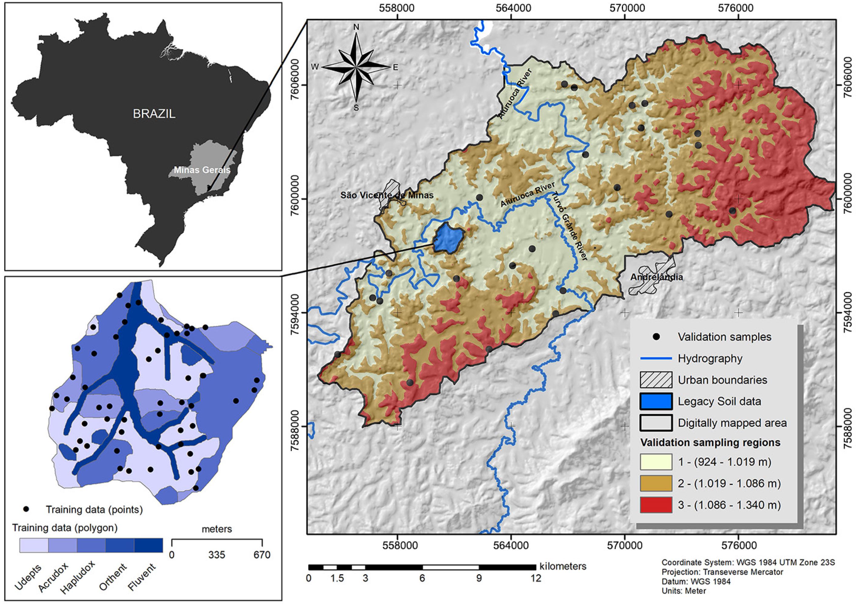
The study area is divided into a reference area, named Vista Bela Creek watershed, wherefrom the legacy data was extracted (175 ha) for model training, and a digitally mapped area (2,719 ha), where a new soil map was generated (Figure 1). Both areas are located in the state of Minas Gerais, Brazil, between latitudes S 21°37’03” and 21°48’67” and longitudes W 44°28’20” and 44°12’98”, 23K, datum WGS 1984, with an elevation range of 924-1342 m. The relief was modeled through intense dissection provided by fluvial erosion, resulting in hilly features with convex to tabular summit and convex slopes, interspersed by elongated crests. There is a predominance of gneisses and biotite-schists of Carrancas sequence and biotite-gneiss and amphibolite of Serra do Turvo sequence. According to the Köppen classification, the climate is Cwa, with dry winter and rainy summer. The mean annual temperature varies between 18 and 22 °C, presenting an annual precipitation average of 1,450 mm (Menezes et al., 2009).

Figure 1
Study areas location: Vista Bela Creek Watershed (soil legacy from reference area) (Menezes et al., 2009) and the digitally mapped area to which information was extrapolated in the state of Minas Gerais, Brazil.

The main soil types found in the area are Udept, Hapludox, Acrudox, and Fluvent (Menezes et al., 2009) according to Soil Taxonomy (Soil Survey Staff, 2014). Orthent has also been found, occurring as inclusions associated with rock outcrops, in an intricate landscape pattern with Inceptisols, which may hinder its individualization, and consequently, the transferability of knowledge.

The soil legacy data consisted of a soil map on a detailed scale (1:10,000) (Menezes et al., 2009). The watershed is considered as a reference area (Favrot, 1989; Voltz et al., 1997), since it comprises all the soil-landscape relationships occurring in the region that can be extrapolated to areas with similar physiographic conditions. The soil map was produced on a traditional basis: analysis of aerial photography and manual delineation of soil mapping units, along with intensive fieldwork (total of 53 soil profiles). This map was used as the source of information for training Random Forest models.

Environmental covariates: relief maps

A digital elevation model (DEM) with 20 m of resolution was generated from contour lines freely available from the Brazilian Institute of Geography and Statistics (IBGE), on a 1:50,000 scale and 20 m of equidistance. A hydrologic consistent DEM was generated in the ArcGIS information system (version 10.1 of ESRI) by the Topo to Raster tool. From the DEM, 14 topographic indexes were created using the SAGA GIS software program (SAGA Development Team version 3.0) and selected due to their capacity to express variations of both morphometrical and hydrological characteristics on local and landscape scales. The following topographic indexes were calculated: catchment slope (CS), convergence index (CI), plan curvature (Plan C) and profile curvature (Prof C) (Zevenbergen and Thorne, 1987), multiresolution index of ridge top flatness (MRRTF) (Gallant and Dowling, 2003), slope, LS-factor (LSF), SAGA wetness index (SWI), topographic position index (TPI) (Guisan et al., 1999), terrain surface texture (Texture) (Iwahashi and Pike, 2007), terrain classification index for lowlands (TCI), upslope curvature (USC), valley depth (VD), vertical distance to channel network (VDCN) and slope.

Training datasets

The complete framework, including the choice of training dataset up to the spatial prediction of soil types of the digitally mapped area, is presented in Figure 2D. The randomForest package (version 4.6-12) in the statistical software R program (R Development Core Team, version 1.0.44) was used. The choice of mtry is often the square root of the number of variables (p); in this case it was 4 and the parameter ntree was adjusted to 1,000. The following approach to using legacy data for training Random Forest was applied:

Figure 2
Flowchart of training data scheme and their interaction with the variables. A) Composition of Point training datasets; B) Development of Polygon training datasets; C) Training data reduction for development of PCA training datasets; D) Summary of the proposed methodology; OOB = out-of-bag; PCA = Principal Component Analysis; Dim = Dimension; RF = Random Forest.

Point legacy data (Figure 2A) comprised: a) 53 soil legacy samples; and b) a circular buffer of 30 m radius around each soil sample point, aiming to increase the number of points with soil information extracted from the raster file to be used by the Random Forest. The buffer increases the size of training dataset, which, in turn, could improve the accuracy of Random Forest prediction (Deng and Wu, 2013).

Polygons of soil mapping units (Figure 2B) comprised: a) pixels from the interior of the polygons eliminating 20 m from their boundaries; and b) pixels from the interior of the polygons eliminating 30 m from their boundaries.

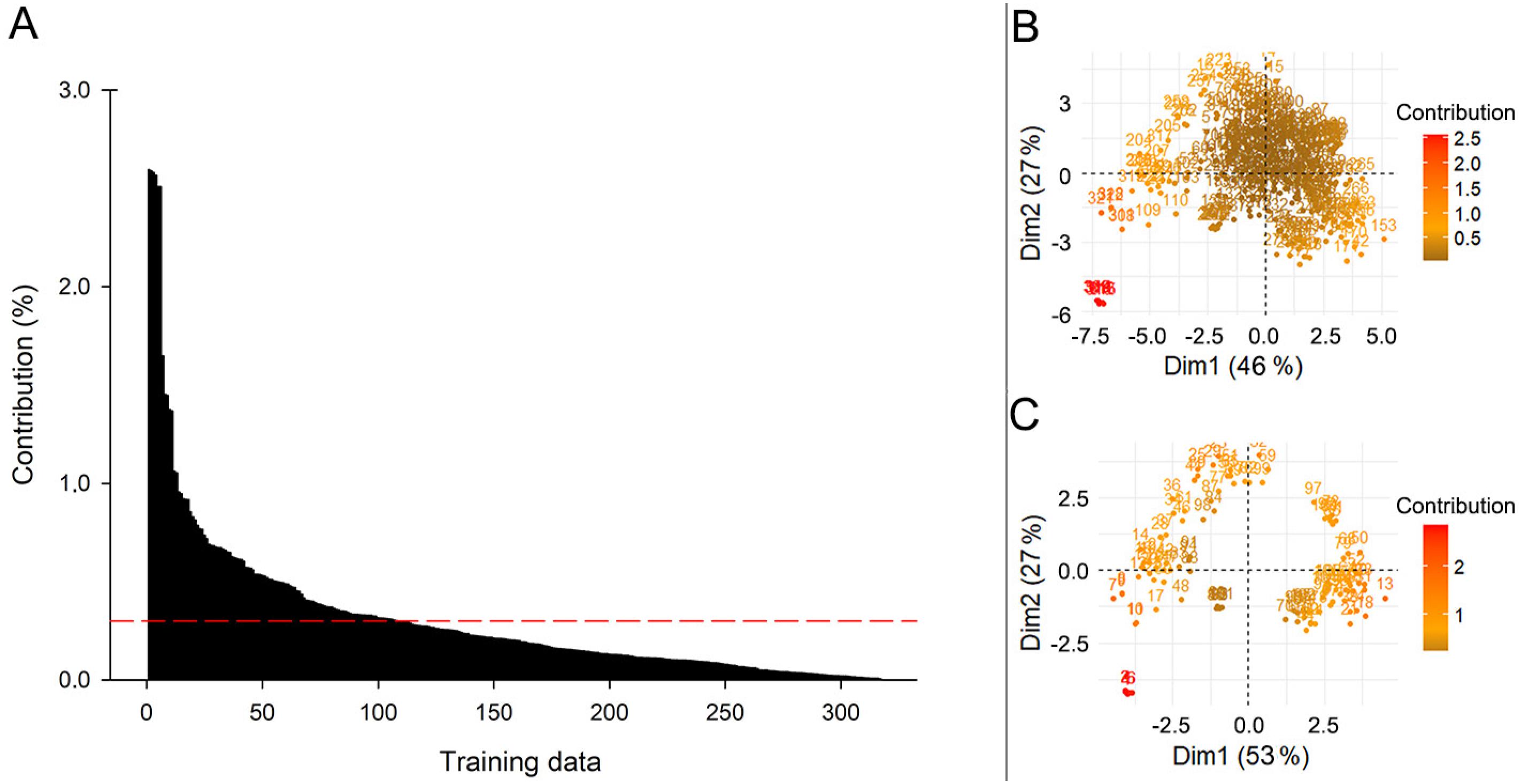
PCA of Polygons and Points training datasets (Figure 2C): PCA was applied (FactoMineR package, version 1.36) by means of the R software environment (R Development Core Team, version 1.0.44). Soil type and topographic covariates were the data analyzed by PCA. Considering that the contribution of the individuals (pixels) to the principal components of a given dataset can be measured, it was possible to reduce the data to a new ensemble more aligned with the variables, according to Figure 3C. The red line in Figure 3A indicates the individuals’ expected average contribution (EAC). For a given component, an observation with a contribution greater than this cutoff could be considered as important in terms of contributing to the component, reducing the subjectivity in explanatory information reduction. Figure 3B shows the variation contribution of the dataset, the closer to the center, the lower the contribution of a given observation. Therefore, the contribution of individuals was calculated for each training dataset described above, and the pixels with values below the EAC were excluded (Figure 3C).| Applying this procedure, four additional training datasets were created, namely PCA-Point, PCA Buffer-Point, PCA Pol −20 m, PCA Pol −30 m.

Figure 3
A) Contribution of individuals to dimensions-1-2 of the principal component analysis for the data set; B) The variation of contribution of the data set; C) Reduction of data dimension; Dim = Dimension.

Variable reduction

Different kinds of tests, in order to assess the effects of variable reduction in spatial prediction (Figure 2D), were developed:

1. The Random Forest classifier was initially loaded with the entire set of predictors (topographical indexes) for each soil information dataset (control).

2. Based on the Random Forest algorithm, the mean decrease in accuracy (MDA) was obtained and the variable importance ranked. For each dataset, the top eleven (MDA11), nine (MDA9) and five (MDA5) variables were selected and a new model was derived.

3. The whole set of soil data and its correspondent terrain indexes was submitted to PCA. The reduction in variables was derived from the expected average contribution of the variables for the dimensions 1-2 of PCA. For the given components, the variables with a contribution lower than this cutoff were excluded (PCA1-2).

4. For each dataset from the dimensions 1-2 of the PCA had the top nine attributes selected from a rank (PCA9).

5. For each dataset, from the dimensions 1-2 of the PCA the top five attributes (PCA5) were selected from a rank.

It is important to highlight that PCA was performed for both reduction of predictor variables and training points. Thus, in the aforementioned procedures 3, 4, and 5, the Random Forest was loaded with the ensemble of variables defined for their original training sets (Figure 2D).

Assessment of the accuracy of predictions within the digitally mapped area

The assessment of DSM accuracy was done using 23 soil profiles (external validation), which was then denominated as the digitally mapped area (Figure 1). The sampling sites were chosen by means of the Regional Random method on ArcSIE (Soil Inference Engine - ArcGIS extension, version 10.3.101). The locations were randomly defined within polygons, representing three altitude levels (sampling regions) as shown in Figure 1. Two indexes were calculated: overall accuracy and the Kappa index. The overall accuracy is the sum of the main diagonal components of the confusion matrix divided by the total of validation samples (in the proportion of correct predicted soil types)

The Kappa index is an agreement measure calculated by taking into account the total number of samples, the number of soil types and the correctly classified samples (Congalton and Green, 2008). The values may range from −1 (suggesting disagreement) to 1 (suggesting excellent agreement) (Landis and Koch, 1977).

User's accuracy and producer's accuracy were also calculated. User's accuracy shows the probability of the predicted class on the map of matching the class in the field, while the producer's accuracy expresses the probability of a soil type point being correctly classified on the map (Congalton, 1991). An accurate map has index values closer to one (100 %) (Behrens et al., 2010).

Prediction uncertainty

The prediction uncertainty was evaluated by vote count and entropy maps. The ensemble-modeling, like Random Forest, has as benefits the possibility of estimating uncertainty by using the vote count surface. In this study, each model corresponds to 1,000 interactions. By the end of the procedure, each pixel receives 1,000 votes. Thus, the range of votes varies from 0 % to 100 %. Pixel values closer to 0 % or 100 % indicate less uncertainty. The higher the value, the greater the certainty of that pixel of corresponding to a given soil type. The lower the value, the higher the certainty of a given pixel not corresponding to a given soil type. Therefore, the values in between this range carry more uncertainty.

To represent the overall uncertainty, the entropy measure (H) was used to describe how the ensemble-model intends its predictions to apply to a particular soil type. It expresses the degree of certainty in a pixel classification in which the votes are concentrated in a particular class, rather than spread over a number of classes (Zhu, 1997). The H values range from 0 to 1, where the higher the H value at a location, the higher the uncertainty of classification.

To better understand the uncertainty in predictions, a landforms map was generated. The DEM was selected as input data to the TPI-based landform classification module on SAGA GIS resulting in ten landform classes in the study area. The derived landform classes were intersected with the vote-count and entropy maps for the interpretation of the uncertainty predictions´ distribution on the landscape.

Results and Discussion

Model evaluation

The out-of-bag (OOB) estimate of error has been varied with a wide range (from 5 to 77 %) (Table 1). This index seems to be mainly driven by the number of observations: the margin of error decreases while the number of observations increases. Such a difference is clear when comparing the models with training datasets derived from points and polygons, the last one showing more observations and less error. As regards the group of polygons, those that were reduced using PCA presented mean OOB values slightly lower than their respective original sets. However, when analyzing the whole models by means of training data reduction, two different groups of OOB estimates of error were found: those with less than 53 and those with more than 105 training data observations, with or without PCA analysis, as seen in Table 1.

Table 1
Accuracy measurements of the models developed from point and polygon data.

Training dataset	Number of observations	Variable selection	Number of variables	OOB estimate error	Overall accuracy*	Kappa Index*
				________________ % ________________
Point	53	Control	14	62	57	0.358
		MDA(11)	11	57	57	0.345
		MDA(9)	9	54	48	0.209
		MDA(5)	5	64	43	0.143
		PCA1-2	11	60	57	0.345
		PCA (9)	9	62	57	0.345
		PCA (5)	5	64	39	0.069
PCA-Point	18	Control	14	77	49	0.110
		MDA(11)	11	72	40	0.110
		MDA(9)	9	56	40	0.093
		MDA(5)	5	55	49	0.159
		PCA1-2	11	67	49	0.110
		PCA (9)	9	67	39	0.100
		PCA (5)	5	50	35	0.004
Buffer-Point	322	Control	14	15	65	0.476
		MDA(11)	11	15	65	0.476
		MDA(9)	9	16	70	0.540
		MDA(5)	5	17	70	0.550
		PCA1-2	11	20	65	0.476
		PCA (9)	9	18	65	0.476
		PCA (5)	5	29	70	0.546
PCA Buffer-Point	105	Control	14	18	61	0.410
		MDA(11)	11	20	61	0.410
		MDA(9)	9	18	61	0.410
		MDA(5)	5	21	48	0.211
		PCA1-2	11	21	65	0.474
		PCA (9)	9	18	61	0.409
		PCA (5)	5	32	83	0.738
Pol −20 m	2,314	Control	14	11	57	0.324
		MDA(11)	11	9	52	0.260
		MDA(9)	9	9	52	0.258
		MDA(5)	5	15	57	0.327
		PCA1-2	**	**	**	**
		PCA (9)	9	15	57	0.337
		PCA (5)	5	25	44	0.158
PCA Pol −20m	714	Control	14	6	50	0.226
		MDA(11)	11	5	57	0.343
		MDA(9)	9	5	66	0.474
		MDA(5)	5	6	61	0.417
		PCA1-2	**	**	**	**
		PCA (9)	9	10	53	0.262
		PCA (5)	5	19	40	0.118
Pol −30 m	1,604	Control	14	8	52	0.267
		MDA(11)	11	8	52	0.256
		MDA(9)	9	9	48	0.191
		MDA(5)	5	12	48	0.207
		PCA1-2	**	**	**	**
		PCA (9)	9	14	57	0.327
		PCA (5)	5	21	44	0.172
PCA Pol −30 m	524	Control	14	6	52	0.262
		MDA(11)	11	6	57	0.343
		MDA(9)	9	6	57	0.335
		MDA(5)	5	8	52	0.254
		PCA1-2	**	**	**	**
		PCA (9)	9	10	53	0.279
		PCA (5)	5	14	44	0.160

• PCA = Principal Component Analysis; OOB = out-of-bag observations;
• ^*
  External validation;
• ^**
  For PCA-1-2, there are no values for the polygons group because only nine variables (Terrain Indexes) reached the expected average contribution; Control = All terrain indexes applied for Random Forest spatial prediction; MDA = Variables reduction by means of Mean Decrease in Accuracy; PCA-Variables reduction by means of Principal Component Analysis.

Such results indicate that Random Forest models were sensitive to variations in training dataset. A larger training dataset is often necessary in order to reduce error (Pal and Mather, 2003), and in this study, such information also brought stability to model errors in training data above 105 observations. However, it is important to highlight that the use of polygons and buffers could bring some uncertainty as regards the soil type, mainly closer to the boundaries or transition zones (Pelegrino et al., 2016; ten Caten et al., 2012; Giasson et al., 2015). Thus, the key point here is will the more accurate models deliver accurate soil maps in the digitally mapped area?

Assessment of the digitally produced map (external validation)

Table 1 presents the overall accuracy and kappa index derived from external validation within the digitally mapped area, to where the information was extrapolated. The Point derived models presented the poorest prediction when compared with the Buffer-Point or Polygons, with or without PCA analysis. Also, an increasing of the number of data observations does not bring significant improvements in accuracy, in disagreement with the OOB estimate error from the model. Polygon derived models presented intermediate Kappa values, ranging from 0.118 to 0.474, while the Point derived models (original and buffer) gave rise to maps with both the lowest and highest accuracy values (Kappa index from 0.004 to 0.738). The map with the highest absolute accuracy came from the PCA Buffer-Point dataset, with 0.738 for the Kappa index and 83 % for overall accuracy.

As long as digital soil mapping techniques attempt to take advantage of a large number of explanatory environmental covariates (McBratney et al., 2003), with a relative small proportion of sampling points, the ability of the Random Forest to deal with high dimensional datasets should be tested. Thus, the reduction in dimensionality by means of PCA analysis (Behrens et al., 2010) or calibration of data set selection (Kuang and Mouazen, 2011) would improve the accuracy of spatial prediction, since the most important subsets are used (Millard and Richardson, 2013). In this study, the use of PCA resulted in a slight improvement only in the overall accuracy of models. Nevertheless, as already mentioned, the PCA Buffer-Point dataset presented the most accurate map out of all 52 prediction models, as evaluated by Kappa index and overall accuracy.

It is possible to observe sizeable variations in accuracy even within the same type of training datasets (Table 1), whose variations are due to the choice of terrain indexes. In order to better understand the effects of terrain indexes or the reduction of variables, Table 2 presents the difference between the overall accuracy of the control (all terrain indexes as an input on Random Forest) and the reduced ensembles of each training dataset. It is expected that where the most important input data are used, accuracy would increase (Strobl et al., 2009; Millard and Richardson, 2013). In this study, in general, variable reduction was not related to increasing accuracy. Millard and Richardson (2015) noted high fluctuations in the importance of the variables, even when the same training data was used. Thus, another way to select the importance of the variables from the Random Forest output should be tested, seeking model stability and accuracy improvement.

Table 2
Difference in overall accuracy of the reduced ensembles of variables in relation to the control for each training dataset.

Variables		Point	PCA-Point	Buffer-Point	PCA Buffer-Point	Pol (-20 m)	PCA-Pol (-20 m)	Pol (-30 m)	PCA-Pol (-30 m)
Ensemble	Number
		________________________________________________________________________________________________ % ________________________________________________________________________________________________
Control	14	57	49	65	61	57	50	52	52
MDA(11)	11	0	-9	0	0	-5	+7	0	+5
PCA-1-2	11	0	0	0	+4	*	*	*	*
MDA(9)	9	-9	-9	+5	0	-5	+16	-4	+5
PCA(9)	9	0	-10	0	0	0	+3	+5	+1
MDA(5)	5	-14	0	+5	-13	0	+11	-4	0
PCA(5)	5	-18	-14	+5	+22	-13	-10	-8	-8

• PCA = principal component analysis;
• ^*
  For PCA-1-2, there are no values for the polygons group because only nine variables (Terrain Indexes) reached the expected average contribution; MDA = Variables reduction by means of Mean Decrease in Accuracy; PCA = Variables reduction by means of Principal Component Analysis.

Only two training datasets (PCA Buffer-point; PCA Pol-20 m) presented at least one model with relevant increases in overall accuracy (higher than 15 % in overall accuracy). No relevant variation or reduction in accuracy was found for the others. Thus, the relationship between the predictive capacity of models and terrain indexes cannot be explained only by the number of predictor variables used in each model. As an example, from the best results obtained for the Buffer-Point dataset, the reduction in variables resulted in a slight or no variation in the accuracy of maps. Moreover, different sets of terrain indexes presented the same overall accuracy for the same dataset (Buffer-Point MDA(5), 70 % and Buffer-Point PCA(5), 70 %, as seen in Table 1).

In accordance with the findings of Heung et al. (2014), in this study, the reduction in variables did not necessarily result in great improvements in accuracy with Random Forest. However, the best result obtained in our study was achieved in the reduction of variables. For the PCA Buffer-Point dataset, by reducing the number of the variables to the five most important ones identified by the PCA, there was a 22 % improvement in the accuracy of the map, in accordance with Table 2. In contrast, for the same training data, using the same predictor variables set size, although defined by MDA, the accuracy of the map was 13 % lower when compared to the control model as seen in Table 2. This result is contrary to those obtained by Behrens et al. (2010), who reported that the unsupervised PCA approach turned out to be the worst technique in terms of selecting optimal features for soil classification.

With regard to the reduction of variables, it is important to note that there is no single method for best ranking classifiers from distinct datasets (Novakovic et al., 2011). Different ranking methods may result in different classifications, as shown in Figure 4A and B. Moreover, a poorly ranked variable that could be considered useless by itself, can afford an expressive performance enhancement when combined with others (Guyon and Elisseeff, 2003). In this study, e.g., for PCA Buffer-Point dataset, the best predictor subset was obtained based on PCA-1-2 ranking, composed of the terrain indexes CS, TPI, TCI, LSF and Slope, whose MDA order of importance were 11^th, 6^th, 7^th, 13^th and 14^th, respectively. Once the accuracy is influenced by the choice of features, the use of many rank indices is reasonable in order to assure that the most accurate subset will be obtained (Novakovic et al., 2011). Another important aspect of identifying the main variables is the time saved in the acquisition and preparation of the database and computational efficiency, if there is interest in applying such models to larger and similar areas (Scarpone et al., 2017; Yu et al., 2016).

Figure 4
Overall variable importance. A) Variable importance based on mean decrease in accuracy; B) Variable importance based on its contribution for the dimensions-1-2 of principal component analysis; Dim = dimensions; CS = Catchment slope; CI = Convergence index; PlanC = Planform curvature; ProfC = Profile curvature; LSF = LS-Factor; MRRTF = Multiresolution index of ridge top flatness; SWI = Saga Topographic Wetness Index; TPI = Topographic Position Index; TCI = Terrain Classification for Low Lands; USC = Upslope Curvature; VD = Valley Depth; VDCN = Vertical Distance to Channel Network.

Having a large training dataset and a numerous ensemble of variables does not necessarily result in accurate predictions, despite the low values in the OOB error rate. Figure 5 shows the relationship between the overall error rate and the OOB estimate of that error rate. A weak correlation between model and external validation was found (R² = 0.1395). Before an extensive sequence of tests on different types of Random Forest training datasets, Millard and Richardson (2015) pointed out that the OOB was not a good indicator of error in highly dimensional datasets, and it seems to be driven mainly by dataset training size, as already discussed. Thus, it is recommended to explore different combinations of predictor variables for a single dataset to load the random forest with the whole covariates ensemble, which may not necessarily result in the most accurate map, as well as to provide an independent validation data set in order to avoid any optimistic bias (Hammond and Verbyla, 1996).

Figure 5
Correlation between variations of the Out of Bag (OOB) estimate of error rate and the overall rate of external validation.

Prediction uncertainty

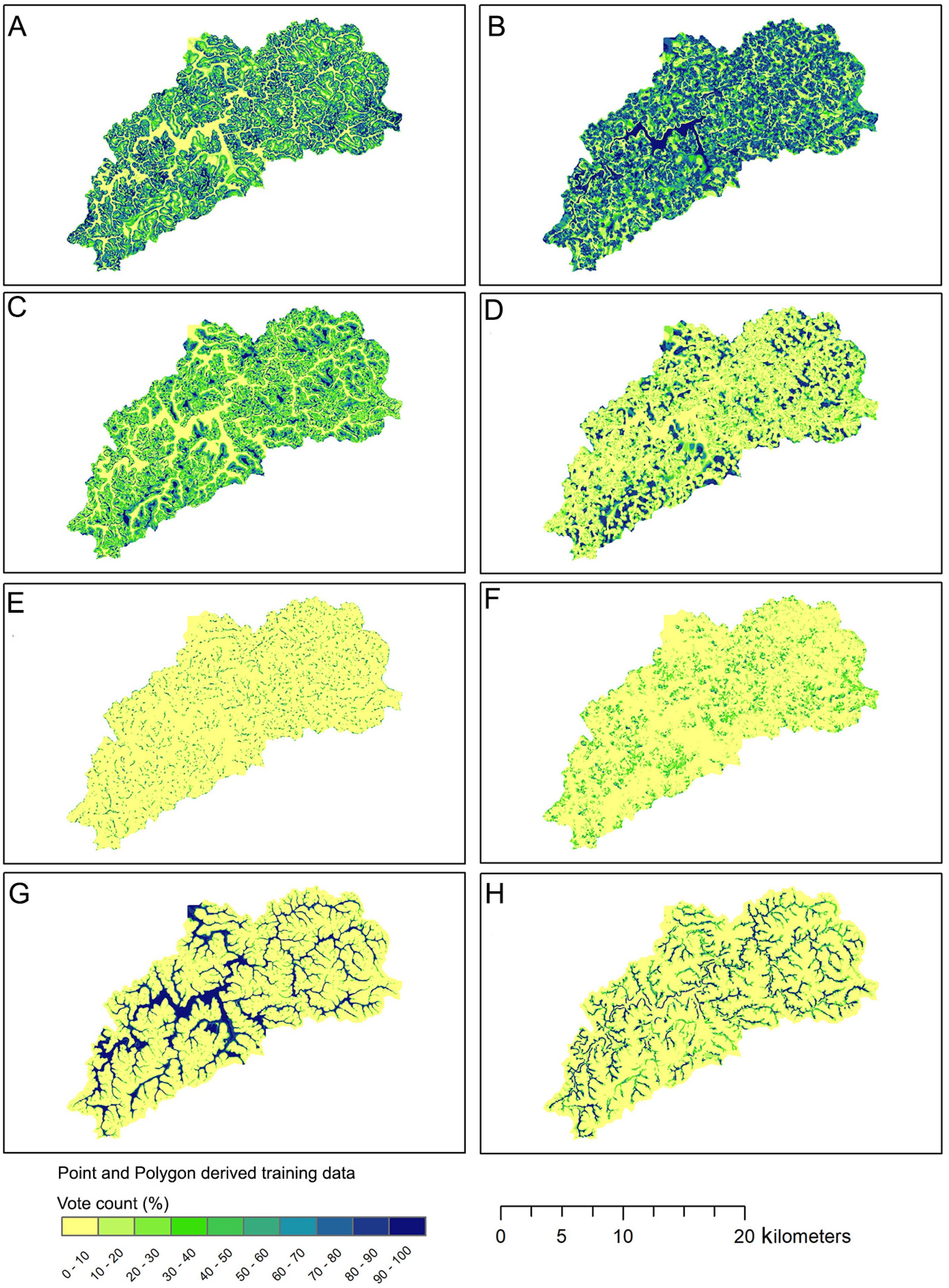
Uncertainty analysis was done in the Random Forest predictions for the two best models obtained (point-derived and polygon-derived training dataset). The vote count surfaces of the soil types are presented in Figure 6A-H. Higher values correspond to areas most likely to harbor a given soil type, and lower values indicate the opposite. Both can be considered areas of low uncertainty. Therefore, intermediate values are indicators of the areas of greatest uncertainty in prediction.

Figure 6
Vote count surfaces on 1000 decision trees of the Random Forest using Point and Polygon derived training data. A) Udept from Point data; B) Udept from Polygon data; C) Hapludox from point data; D) Hapludox from polygon data; E) Acrudox from point data; F) Acrudox from polygon data; G) Fluvents from point data; H) Fluvents from polygon data.

There have been substantial differences when comparing the vote count surfaces from point-derived training data and polygon-derived training data. The latter seems to oversize the certainty area for the probability of the presence of Udepts, advancing forward areas where Fluvents would be expected. Despite this, the producer's accuracy for this class was 50 %, demonstrating that, in addition to oversizing, spatialization was also impaired. For the Oxisols (Acrudox and Hapludox), the general spatialization pattern was considered similar to that of the point-derived model. However, the dimensionalization may be overestimated since the producer's accuracy (84 % and 100 %) was greater than the user's accuracy (63 % and 50 %) for the soil type map. The model derived from the polygons was also less efficient in discriminating Fluvents compared to the point-derived one (Figure 6G and H).

Great extensions of uncertainty over areas of Udepts and Hapludox votes surface maps were found for the point-model compared to the polygon-model. This effect may come from the least amount of training data for the point dataset, which was respectively 8.4 and 2.4 times greater for polygon derived model. However, both soil types presented satisfactory values of both the producer's accuracy and the user's accuracy (Table 3). In this case, the greatest uncertainty was found in Acrudox spatial prediction.

Table 3
Producer's and user's accuracy for the highest accuracy spatial prediction from buffer of point and polygon data.

Dataset	Variables	Udept	Acrudox	Hapludox	Fluvent
		Producer's accuracy
		________________________________ % ________________________________
PCA POL-20	MDA(9)	50	100	84	50
PCA Buffer-Point	PCA(5)	80	0	88	100
		User's accuracy
		____________________________ % ____________________________
PCA POL-20	MDA(9)	78	50	63	25
PCA Buffer-Point	PCA(5)	89	0	88	100

• PCA POL-20 = Training data derived from polygon −20 m dataset and reduced by Principal Component Analysis; PCA Buffer-Point = training data derived from Buffer-Point dataset and reduced by Principal Component Analysis; MDA(9) = the best nine variables of the Mean Decrease in Accuracy rank; PCA(5) = the five variables that most contributed to the Principal Component Analysis.

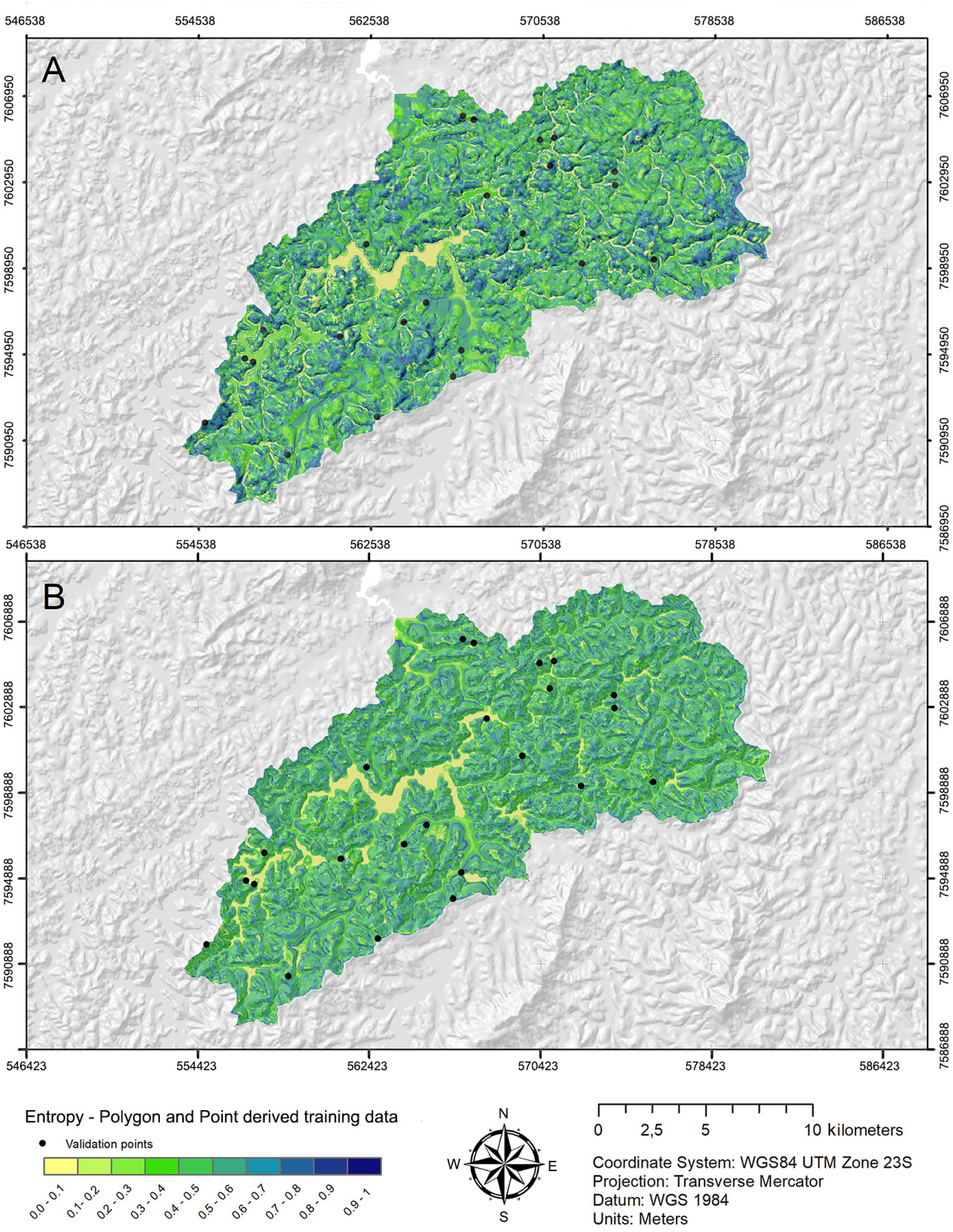
The overall uncertainty prediction was represented by entropy (Figure 7A and B). Polygon and Buffer-Point presented quite similar results: for the polygon-derived models the entropy ranged from 0 to 0.99, with an average of 0.478 and standard deviation of 0.198; for the Buffer-Point derived models the entropy also ranged from 0 to 0.99, with an average of 0.467 and standard deviation of 0.169. Contrary to what was observed by Heung et al. (2017), there was no major difference in the spatial distribution of the overall uncertainty over the study area, considering the different datasets.

Figure 7
Uncertainty surface based on Random Forest model using Point and Polygon-derived training data produced at a 20 m spatial resolution for the study area. A) Entropy values for Polygon derived training data; B) Entropy values for Point-derived training data.

Figure 8 shows the relative frequency distribution of uncertainty related to landforms. In general, the uncertainty was low for valley bottom regions, where there is a predominance of Fluvents occurring over flatter areas around the drainage network, having been formed by the accumulation of sediments from flood deposits. Such values were also found in flat ridge tops and plains, commonly associated with Hapludox.

Figure 8
Overall relative frequency distribution of the entropy values related to the TPI based landforms classification. Streams = canyons and deeply incised streams; Drainages = midslope drainages, shallow valleys, upland drainages and headwaters; Valleys = U-shape valleys; Slopes = open slopes and upper slopes; Ridges = local ridges/hills in valleys, midslope ridges, small hills in plains and high ridges.

In sites where the slope is greater than 20 %, the entropy values ranged from low to intermediate. The steeper the slope, the lower the uncertainty. Such sites are commonly associated with the incidence of Inceptisols. In the region of the study area, this soil type tends to be located in a wide range of slope gradient (3 % to 45 %).

Higher uncertainty was found in footslopes and convex ridges. The former is probably related to the common associations between Udepts and Hapludox in this region, which can generate “confusion” when discriminating the domains of each type of soil. Silva et al. (2016) reported an analogous condition studying a nearby area, where in similar landscape positions both Inceptisols and Oxisols are found. Inceptisols tend to lie in the upper third and sometimes in the inferior third of the backslope in association with Oxisols (Curi et al., 1994). In relation to the convex ridges, higher values of uncertainty may be due to the difficulty in telling the domains of Hapludox, Acrudox, and occasionally Udepts apart. Such pattern of soil distribution was a common situation in the northeastern portion of the study area.

Most of the models presented low accuracy for Acrudox (Table 3) along with greater uncertainty, as observed in Figures 7A and B. This is related mainly to two factors: a) the low density of the training and validation datasets, since such soil type has low geographical expression in this region when compared with the others. This relative imbalance tends to favor the majority classes within the training dataset (He and Garcia, 2009). In other words, classes overrepresented in the training dataset may dominate classification by the model (Millard and Richardson, 2015). This natural imbalance is common when dealing with soil type distribution. In the reference area (Vista Bela Creek Watershed), Acrudox corresponds to only 12 % of the total area. The same was observed during the field work for the digitally mapped area, where unlike Hapludox, the Acrudox are not found in large contiguous areas, but rather, in transitions between Hapludox areas. Even though the relief explained most of the spatial variability of soil types, it seems that specifically for Acrudox, it is mainly driven by parent material instead of solely relief. Terrain indexes do not efficiently tell the Acrudox and Hapludox areas apart, since both occur in similar portions in the landscape. Since digital soil mapping techniques are updatable (Hengl et al., 2014), the availability of data in the future related to parent material in the same scale of this study could provide improvements in spatial prediction accuracy.

Conclusions

By executing the Buffer, the point-derived data yielded better results compared to Polygon-derived models. Excluding the Buffer and PCA Buffer datasets, there were no significant differences between the accuracy of the models. The reduction of variables was able, in a general way, to improve the accuracy in the predicted maps of soil types, the same as for training data selection. The best result was obtained by identifying the principal components of the Buffer dataset, and reducing the size of the ensemble of predictors with the PCA. Although the uncertainty was relatively similar for both Buffer-Point and Polygon derived models, the one derived from Polygons seems to have introduced more noise into the models, as observed by inconsistencies in the spatial prediction of soil types. The natural imbalance in the dataset training related to soil types with smaller geographical expression could underrepresent its spatial prediction from the Random Forest and increase the uncertainty in certain types, such as Acrudox in the region of the study.

Even though the Random Forest has been considered a robust spatial predictor model in Soil Science, its sensitivity to different strategies of selecting training dataset is very clear. Effort was necessary to find the best training dataset for achieving suitable accuracy of spatial prediction. To identify a specific dataset in this study seems to be preferable than a large number of variables or a large size of training data. Thus, the efforts here allowed the for the accurate acquisition (83 % for overall accuracy and 0.738 for Kappa index) of a mapped area (2,719 ha) 15.5 times greater than the reference area (175 ha), up to the second hierarchical level according to Soil Taxonomy, at low cost by taking advantage of soil legacy data.

Acknowledgments

The authors thank the funding agency Coordenação de Aperfeiçoamento de Pessoal de Nível Superior (CAPES) and Conselho Nacional de Desenvolvimento Científico e Tecnológico (CNPq) (137672/2015-2) for providing financial support by means of a scholarship for the development of this work.

References

• Arruda, G.P.; Demattê, J.A.M.; Chagas, C.S.; Fiorio, P.R.; Souza, A.B.; Fongaro, C.T. 2016. Digital soil mapping using reference area and artificial neural networks. Scientia Agricola 73: 266-273.
• Behrens, T.; Zhu, A.-X.; Schmidt, K.; Scholten, T. 2010. Multi-scale digital terrain analysis and feature selection for digital soil mapping. Geoderma 155: 175-185.
• Breiman, L. 2001. Random forests. Machine Learning 45: 5-32.
• Chagas, C.S.; Carvalho Junior, W.; Bhering, S.B.; Calderano Filho, B. 2016. Spatial prediction of soil surface texture in a semiarid region using random forest and multiple linear regressions. Catena 139: 232-240.
• Congalton, R.G. 1991. A review of assessing the accuracy of classifications of remotely sensed data. Remote Sensing of Environment 37: 35-46.
• Congalton, R.G.; Green, K. 2008. Assessing the Accuracy of Remotely Sensed Data: Principles and Practices. 2ed. CRC Press, Boca Raton, FL, USA.
• Curi, N.; Chagas, C.S.; Giarola, N.F.B. 1994. Distinction of agricultural environments and soil-pasture relationship in the Mantiqueira fields = Distinção de ambientes agrícolas e relação solo-pastagens nos campos da Mantiqueira. p. 21-43. In: Carvalho, M.M.; Evangelista, A.R.; Curi, N., eds. Pasture growth in the Campos das Vertentes physiographic zone = Desenvolvimento de pastagens na zona fisiográfica Campos das Vertentes, MG. ESAL, Lavras, MG, Brazil (in Portuguese).
• Deng, C.; Wu, C. 2013. The use of single-date MODIS imagery for estimating largescale urban impervious surface fraction with spectral mixture analysis and machine learning techniques. ISPRS Journal of Photogrammetry and Remote Sensing 86: 100-110.
• Favrot, J.C. 1989. A strategy for large scale soil mapping: the reference areas method. Science du Sol 27: 351-368 (in French, with abstract in English).
• Gallant, J.C.; Dowling, T.I. 2003. A multiresolution index of valley bottom flatness for mapping depositional areas. Water Resources Research 39: 1347-1359.
• Giasson, E.; ten Caten, A.; Bagatini, T.; Bonfatti, B. 2015. Instance selection in digital soil mapping: a study case in Rio Grande do Sul, Brazil. Ciência Rural 45: 1592-1598.
• Grinand, C.; Arrouays, D.; Laroche, B.; Martin, M.P. 2008. Extrapolating regional soil landscapes from an existing soil map: sampling intensity, validation procedures, and integration of spatial context. Geoderma 143: 180-190.
• Guisan, A.; Weiss, S.B.; Weiss, A.D. 1999. GLM versus CCA spatial modeling of plant species distribution. Plant Ecology 143: 107-122.
• Guyon, I.; Elisseeff, A. 2003. An introduction to variable and feature selection. Journal of Machine Learning Research 3: 1157-1182.
• Hammond, T.O.; Verbyla, D.L. 1996. Optimistic bias in classification accuracy assessment. International Journal of Remote Sensing 7: 1261-1266.
• Hastie, T.; Tibshirani, R.; Friedman, J. 2009. The Elements of Statistical Learning: Data Mining, Inference, and Prediction. 2ed. Springer, New York, NY, USA.
• He, H.; Garcia, E. 2009. Learning from imbalanced data. IEEE Transactions on Knowledge and Data Engineering 21: 1263-1284.
• Hengl, T.; Heuvelink, G.B.M.; Kempen, B.; Leenaars, J.G.B.; Walsh, M.G.; Shepherd, K.; Sila, A.; MacMillan, R.A.; Jesus, J.M.; Tamene, L.; Tondoh, J.E. 2015. Mapping soil properties of Africa at 250 m resolution: random forests significantly improve current predictions. Plos One 10: e0125814.
• Hengl, T; Jesus, J.M.; MacMillan, R.A.; Batjes, N.H.; Heuvelink, G.B.M.; Ribeiro, R.; Samuel-Rosa, A.; Kempen, B.; Leenaars, J.G.B.; Walsh, M.G.; Gonzalez, M.R. 2014. SoilGrids1km - global soil information based on automated mapping. Plos One 9: e114788.
• Heung, B.; Bulmer, C.E.; Schmidt, M.G. 2014. Predictive soil parent material mapping at a regional-scale: a random forest approach. Geoderma 214-215: 141-154.
• Heung, B.; Ho, H.C; Zhang, J.; Knudby, A.; Bulmer, C.E.; Schmidt, M.G. 2016. An overview and comparison of machine-learning techniques for classification purposes in digital soil mapping. Geoderma 265: 62-77.
• Heung, B.; Hodúl, M.; Schmidt, M.G. 2017. Comparing the use of training data derived from legacy soil pits and soil survey polygons for mapping soil classes. Geoderma 290: 51-68.
• Iwahashi, J.; Pike, R.J. 2007. Automated classifications of topography from DEMs by an unsupervised nested means algorithm and a three-part geometric signature. Geomorphology 86: 409-440.
• Jenny, H. 1941. Factors of Soil Formation: A System of Quantitative Pedology. McGraw-Hill, New York, NY, USA.
• Kempen, B.; Brus, D.J.; Stoorvogel, J.J.; Heuvelink, G.B.M.; Vries, F. 2012. Efficiency comparison of conventional and digital soil mapping for updating soil maps. Soil Science Society of America Journal 76: 2097-2115.
• Kuang, B.; Mouazen, A.M. 2011. Calibration of visible and near infrared spectroscopy for soil analysis at the field scale on three European farms. European Journal of Soil Science 62: 629-636.
• Lagacherie, P.; Legros, J.P.; Burrough, P.A. 1995. A soil survey procedure using the knowledge of soil pattern established on a previously mapped reference area. Geoderma 65: 283-301.
• McBratney, A.B.; Santos, M.L.M.; Minasny, B. 2003. On digital soil mapping. Geoderma 117: 3-52.
• McKay, J.; Grunwald, S.; Shi, X.; Long, R. 2010. Evaluation of the transferability of a knowledge-based soil-landscape model. p. 165-178. In: Boettinger, J.L.; Howell, D.W.; Moore, A.C.; Hartemink, A.E.; Kienast-Brown, S., eds. Digital soil mapping progress in soil science. Springer, Dordrecht, The Netherlands.
• Mendonça-Santos, M.L.; Santos, H.G. 2007. The state of the art of Brazilian soil mapping and prospects for digital soil mapping. p. 39-54. In: Lagacherie, P.; McBratney, A.B.; Voltz, M., eds. Developments in soil science. Elsevier, Amsterdam, The Netherlands.
• Menezes, M.D.; Curi, N.; Marques, J.J.; Mello, C.R.; Araújo, A.R. 2009. Pedologic survey and geographic information system for evaluation of land use within a small watershed, Minas Gerais state, Brazil. Ciência e Agrotecnologia 33: 1544-1553 (in Portuguese, with abstract in English).
• Millard, K.; Richardson, M. 2013. Wetland mapping with LiDAR derivatives, SAR polarimetric decompositions, and LiDAR-SAR fusion using a RF classifier. Canadian Journal of Remote Sensing 39: 290-307.
• Millard, K.; Richardson, M. 2015. On the importance of training data sample selection in random forest image classification: a case study in peatland ecosystem mapping. Remote Sensing 7: 8489-8515.
• Novakovic, J.; Strbac, P.; Bulatovic, D. 2011. Toward optimal feature selection using ranking methods and classification algorithms. Yugoslav Journal of Operations Research 21: 119-135.
• Pal, M.; Mather, P.M. 2003. An assessment of the effectiveness of decision tree methods for land cover classification. Remote Sensing of Environment 86: 554-565.
• Pelegrino, M.H.P.; Silva, S.H.G.; Menezes, M.D.; Silva, E.; Owens, P.R.; Curi, N. 2016. Mapping soils in two watersheds using legacy data and extrapolation for similar surrounding areas. Ciência e Agrotecnologia 40: 534-546.
• Rudiyanto, R.; Minasny, B.; Setiawan, B.I.; Arif, C.; Saptomo, S.K.; Chadirin, Y. 2016. Digital mapping for cost-effective and accurate prediction of the depth and carbono stocks in Indonesian peatlands. Geoderma 272: 20-31.
• Samuel-Rosa, A.; Heuvelink, G.B.M.; Vasques, G.M.; Anjos, L.H.C. 2015. Do more detailed environmental covariates deliver more accurate soil maps? Geoderma 243-244: 214-227.
• Scarpone, C.; Schmidt, M.G.; Bulmer, C.E.; Knudby, A. 2017. Semi-automated classification of exposed bedrock cover in British Columbia's southern mountains using a random forest approach. Geomorphology 285: 214-224.
• Silva, S.H.G.; Menezes, M.D.; Owens, P.R.; Curi, N. 2016. Retrieving pedologist's mental model from existing soil map and comparing datamining tools for refining a larger area map under similar environmental conditions in southeastern Brazil. Geoderma 267: 65-77.
• Soil Survey Staff. 2014. Keys to Soil Taxonomy. 12ed. USDA-Natural Resources Conservation Service, Washington, DC, USA.
• Souza, E.; Fernandes Filho, E.I.; Schaefer, C.E.G.R.; Batjes, N.H.; Santos, G.R.; Pontes, L.M. 2016. Pedotransefer functions to estimate bulk density from soil properties and environmental covariates: Rio Doce basin. Scientia Agricola 73: 525-534.
• Strobl, C.; Malley, J.; Tutz, G. 2009. An introduction to recursive partitioning: rationale, application and characteristics of classification and regression trees, bagging and RF. Psychological Methods 14: 323-348.
• ten Caten, A.; Dalmolin, R.S.D.; Ruiz, L.F.C. 2012. Digital soil mapping: strategy for data pre-processing. Revista Brasileira de Ciência do Solo 36: 1083-1091.
• Voltz, M.P.; Lagacherie, P.; Louchart, X. 1997. Predicting soil properties over a region using sample information from a mapped reference area. European Journal of Soil Science 48: 19-30.
• Yu, L.; Fu, H.; Wu, B.; Clinton, N.; Gong, P. 2016. Exploring the potential role of feature selection in global land-cover mapping. International Journal of Remote Sensing 37: 5491-5504.
• Zevenbergen, L.W.; Thorne, C.R. 1987. Quantitative analysis of land surface topography. Earth Surface Processes and Landforms 12: 47-56.
• Zhu, A.X. 1997. A similarity model for representing soil spatial information. Geoderma, 77: 217-242.

Edited by

Edited by: Silvia del Carmen Imhoff

Publication Dates

• Publication in this collection
  May-Jun 2019

History

• Received
  23 Aug 2017
• Accepted
  17 Jan 2018