Identification of patterns for increasing production with decision trees in sugarcane mill data

ABSTRACT:

Sugarcane mills in Brazil collect a vast amount of data relating to production on an annual basis. The analysis of this type of database is complex, especially when factors relating to varieties, climate, detailed management techniques, and edaphic conditions are taken into account. The aim of this paper was to perform a decision tree analysis of a detailed database from a production unit and to evaluate the actionable patterns found in terms of their usefulness for increasing production. The decision tree revealed interpretable patterns relating to sugarcane yield (R² = 0.617), certain of which were actionable and had been previously studied and reported in the literature. Based on two actionable patterns relating to soil chemistry, intervention which will increase production by almost 2 % were suitable for recommendation. The method was successful in reproducing the knowledge of experts of the factors which influence sugarcane yield, and the decision trees can support the decision-making process in the context of production and the formulation of hypotheses for specific experiments.

Keywords:
data mining; yield variability; regression tree; knowledge discovery

Introduction

The sugarcane (Saccharum spp.) industry sector, following the evolution of information technologies, has benefited from the automation of processes associated with the collection and storage of data during their normal operation. These processes thus generate databases related to production and factors that can influence the industry, including those at the commercial block level, which is the smallest administrative unit of commercial fields. According to Lawes and Lawn (2005), these large databases have shown a wide range of uses, including predictions of production – as a basis for seasonal planning – and identification of the soil, climate, and management factors that affect yield. The main advantage of analysing databases of production areas is that they represent what actually occurred at the commercial level and capture, on a large scale, a wide range of interactions between factors, which is difficult to accomplish through experimentation in the field.

Furthermore, research on the interaction of genotype × management × environment with sugarcane yield and sugarcane ratoon yield decline has shown that management and weather conditions are more influential than genotype (Ramburan et al., 2011). However, studies that simultaneously analyse variables related to different varieties, climate, detailed management, and edaphic conditions are still rare (Ellis et al., 2001; Ferraro et al., 2009; Lawes et al., 2002). Such data sets with greater availability of attributes relating to the production system lead to a better description of the system, and improve the knowledge that can be obtained from such data (Zhang et al., 2005; 2006).

Taking into account the complexity of the available databases and the focus on identifying patterns that will increase production, the decision tree modeling technique can be adopted, since it has already been successfully applied to several other crops to describe the factors that influence yield (De'ath and Fabricius, 2000; Ferraro et al., 2009; 2012; Zhang et al., 2005; Zheng et al., 2009). We refer to Hastie et al. (2009) for further details about decision trees.

In this paper, we discuss how we performed an analysis using a decision tree of a detailed database from a sugarcane mill and evaluated the usefulness of actionable patterns found in increasing production.

Materials and Methods

The production unit under study is in Teodoro Sampaio, in the state of São Paulo, Brazil (22°31’ S, 52°10’ W, altitude 321 m). The supplied commercial block records for the production and ripening of sugarcane correspond to the seasons 2010/11 and 2011/12 and represent a harvested area of approximately 25,000 ha per season, with an average block size of 22.6 ha. The climate in this region is characterized as suitable for rain-fed sugarcane with an annual water deficit between 10 and 40 mm, mean daily temperature between 20 and 24 °C, and mean daily temperature of the coldest month above 17 °C. The weather for the period evaluated is shown in Figure 1.

Figure 1
Monthly precipitation (mm) and average monthly temperature (°C) for the Sugarcane Mill under study, in Teodoro Sampaio, in the state of São Paulo, Brazil (22°31’ S, 52°10’ W, altitude 321 m), from Jan 2010 to Nov 2012.

The studied sugarcane production system was non-irrigated. Nitrogen and potassium fertilization was applied from the second cut onwards, and phosphorus input was applied in planting furrows only. The planting system was mechanized in 89 % of the blocks, and 98 % were mechanically harvested (green cane). The main varieties planted were RB86 7515 (47 %), SP81 3250 (13 %), and SP80 1842 (9 %).

The database used has 2,255 entries, each corresponding to a commercial block, 68 predictor attributes, and sugarcane yield (Y) as the target attribute, given in tons of sugarcane per hectare. The predictors available in the data set are related to the soil texture in three layers (0-25, 25-50, and 80-100 cm), the clay gradient between the 25-50 and 0-25-cm layers, soil analysis (P, K, Ca, P, pH, sum of bases, base saturation, cation exchange capacity [CEC], organic matter, Al, H+Al, Al saturation), and management practices (fertilization rates, vinasse and filter cake application, variety, and number of cuts). Soil analysis was also used to derive a number of relationships between different nutrients, namely Ca/Mg, Ca/K, Mg/K, K/CEC, and K/(Ca + Mg)½. Additional information was included, such as the season in which there was a harvest (fall, winter, or spring) and occurrence of frost. Detailed information about predictors is provided in ^Appendix1.

The climate was divided into four phenological phases throughout the sugarcane development cycle: sprouting (phase I), tillering (phase II), growth (phase III), and ripening (phase IV). This climate segmentation aimed to represent the different effects on each of the crop growth phases (Binbol et al., 2006). Because of the lack of data on phenology, estimates were based on the typical local behavior of the crop, which was subsequently validated by the technical team of the production unit. Sugarcane planted from Feb till mid-Apr was classified as an 18-month cycle, with sprouting lasting for one month if planted in Feb and Mar, and two months if planted in Apr. Tillering lasted for three months. The grand growth phase was assumed to last until Feb if the cane was harvested in Mar or until Feb if harvested later. The last phase was ripening. For sugarcane planted in the second half of Apr until Aug, sprouting was assumed to last two months, tillering three months, grand growth six months, and ripening two months. Sugarcane planted between Sept and Jan was classified as a 12-month cycle, with two months of sprouting, except for planting in Jan, when it lasted for one month. Tillering lasted for three months, and the grand growth lasted until two months before harvest. These last two months were considered the ripening phase. For ratoon sugarcane (the crop that grows from stubbles following harvest), sprouting was assumed to last one month and tillering three months. Ripening was assumed to last one month if harvesting was in Feb, Mar, or Apr; two months if the harvest was in May, June, or July; and three months for the remainder of the season.

Since sugarcane is planted all year round in the region under study, each possible planting date was simplified and segmented into three periods according to crop cycle duration and the associated weather: 18-month-old (blocks planted from Feb to first half of Apr), 15-month-old (planting from second half of Apr to Aug), and 12-month-old planting (from Sept to Jan). From the second cut onward, blocks were considered ratoon cane. All statistical analyses were undertaken using JMP/SAS version 11.2.

The decision tree was applied to explain the variation of a target attribute by explanatory variables, which means, in the case of this study, explaining the sugarcane yield by the 68 predictor attributes. The decision tree was constructed by repeated binary splitting of the database, defined by a simple rule – type IF… THEN – based on a single predictive attribute. At each split (called node), the database was segmented into two groups in order to reduce the variance of the target attribute as much as possible. In other words, at each node, all predictive attributes were ranked based on their capacity to reduce the target attribute variability, and the best one was used to split the data.

When the predictive attribute is categorical, all possible combinations of its levels in two groups were tested and the best combination was used to rank the predictive attribute among all others. If the predictive attribute was continuous, it was split into two groups through a cutting point (values below and above this cutting value). All possible cutting points were tested and the best was utilized.

The splitting procedure continued to be applied automatically by the decision tree algorithm to each group separately until a stopping parameter, which had been previously defined by the user, was reached. For all splits all explanatory variables are automatically tested by the algorithm, which then selects the one that minimizes the variance of the two resulting database groups.

The aim of the decision tree is to partition the response into homogeneous groups, but also to keep the tree reasonably small, through stopping rules, in order to facilitate its interpretation. The two stopping rules established were the minimum number of records per leaf equal to 40 and the minimum adjusted p-value for the division of 0.1 %. The decision tree was represented graphically with the root node, which represents the unpartitioned data, on the left-hand side, and the nodes and leaves (each leaf represents one of the final database groups) on the right-hand side.

The decision tree can be used for automatic knowledge extraction from data sets that are too voluminous for manual analysis, discovering interactions between predictors, dealing with several types of data (categorical and numerical), and working with non-linearity and threshold-dependent responses. When the target attribute is numeric, decisions trees are often called regression trees. We maintained the use of decision trees in this paper even though our target attribute was numeric.

It is important to highlight two limitations of the decision tree technique. First, there is no possibility of expressing linear relations in a simple and concise way similar to linear regression. Second, there is no single solution (Zhang et al., 2005). Such advantages and disadvantages make the nature of the decision tree technique a method that is complementary to other techniques.

The model was developed in a training subset (two-thirds of the data, n = 1493) and evaluated in a test subset (one-third, n = 762). Since the stopping rules are set to avoid a complex tree, this procedure should also prevent a model excessively specialized in the training set and incapable of repeating the performance in the test set (overfitting). As a reference to be compared to the decision tree, a multiple linear regression with a stepwise automated variable selection procedure was generated. The 10 % level of significance was used to determine the selection of variables as predictors.

For certain rules extracted from the induced tree, we evaluated how much the yield could be increased based on the pattern found. For an arbitrary split, there will be leaves with lower yield (LY) and leaves with higher yield (HY), corresponding to different areas with lower yield (SLY) and areas with higher yield (SHY). Assuming that the pattern was actionable, we evaluated the potential to bring the area under LY conditions to HY conditions. This changed the yield from the node from $\text{LY*SLY}+\text{HY*SHY}$ to $\text{HY}(\text{SLY}+\text{SHY})$. Using data from two years, the evaluation was carried out based on the area under conditions for LY and HY in the different years, and the production was averaged.

Results

The decision tree generated (Figure 2) had 16 leaves and explained 61 % of the variability in the data (for training set R² = 61 %), with 12 significant attributes. By comparison, the multiple linear regression method was able to explain 62 % of the variability, but with 37 significant attributes.

Figure 2
Decision tree for the analysis of factors of influence on the sugarcane yield (Y = mean ± standard error; N = number of records on the leaf; L# = leaf number; N# = node number). In each rectangle, in the top row, the most significant variable selected and the cut-off point (the value of the variable in which the division is made) are given; on the central line, the value represents the mean ± standard error of sugarcane yield; and, on the bottom line, the number of blocks that satisfies this condition is given. The tree should be interpreted from left to right, up to the leaves (rightmost boxes, in gray). In the initial splits, consecutive nodes were created by the same predictor attribute, and the tree was simplified in order to reduce one level and to represent the division into four branches instead of two.

The most important factor was the number of cuts. This parameter was divided into four groups: 15- and 18-month-old plant cane, with an average yield of 84.3 t ha⁻¹; 12-month-old plant cane (Y = 72.3); second cut ratoon cane (Y = 67.2); and ratoon cane from the third cut onwards (Y = 49.3).

For the group of number of cuts for 15- and 18-month-old sugarcane plants, the calcium content in the soil was found to have the greatest influence in yield (Figure 2, N1), in which areas with values below 7 mmol_c dm⁻³ had a lower yield (Figure 2, L2) of 79.9 t ha⁻¹ compared to the yield of 85.7 t ha⁻¹ in the areas with calcium contents greater than or equal to 7 mmol_c dm⁻³ (Figure 2, L1).

The average minimum temperature in the third stage of development of the crop (growth) was the most influential factor for the number of cuts for 12-month-old plants. The critical value was 15.6 °C, and the average yield 75.2 t ha⁻¹ for the blocks developed under the condition of a temperature greater than or equal to this critical level (L3). In conditions of lower thermal availability (L4), the average yield was equal to 63.7 t ha⁻¹.

In the second-cut group, the soil chemistry also showed a significant influence. When the Ca/Mg ratio was below 2.67, the average yield was 70.9 t ha⁻¹. When the ratio was equal to or greater than 2.67, the average yield was 64.0 t ha⁻¹, and this node was subdivided once due to the potassium content. When the potassium content was greater than or equal to 1.5 mmol_c dm⁻³ (L6), the yield was 71.2 t ha⁻¹. When the potassium content was below 1.5 mmol_c dm⁻³ (L7), the average yield was equal to 62.5 t ha⁻¹.

Finally, within the group of number of cuts greater than or equal to three, a clay content in the topsoil (0 to 25 cm) greater than or equal to 24 % was associated with areas with higher yields (58.1 t ha⁻¹) when compared with levels of clay below 24 % (46.2 t ha⁻¹). Within this sub-group of more clayey soil, the number of cuts again determined the segmentation in the groups equal to the third cut (L8) (average yield equal to 65.9 t ha⁻¹) and greater than or equal to the fourth cut (L9) (average yield equal to 52.8 t ha⁻¹). In the sub-group with clay content in the topsoil below 24 %, which corresponded to 38 % of the total blocks of the sugarcane mill, the number of cuts was also the factor of greatest influence, where clay content in the topsoil separates the number of cuts equal to or greater than six and the number of cuts from three to five. Under these conditions of six and seven cuts, average daily precipitation greater than or equal to 4.7 mm d⁻¹ (L15) and below this value (L16) in the grand growth stage of development led to average yields equal to 40.0 and 35.1 t ha⁻¹, respectively.

An average minimum temperature greater than or equal to 19.6 °C in the grand growth stage and fertilization with nitrogen were the factors of influence on the conditions of the sub-group of number of cuts from three to five in soils with clay content in the topsoil below 24 %. For N fertilizer rates greater than or equal to 70 kg N ha⁻¹ (L10), the average yield was 61.8 t ha⁻¹. In the situations of fertilization with nitrogen below 70 kg N ha⁻¹, the average yield was 52.4 t ha⁻¹ (L11). For the average minimum temperature in the stage of grand growth below 19.6 °C, the average daily precipitation during the grand growth stage was the next factor used for splitting the tree. When the precipitation was greater than or equal to 5.3 mm d⁻¹ (L12), the average yield was 49.7 t ha⁻¹; if it was below 5.3 mm d⁻¹, there was a new division according to the sand content in the second layer of the soil (25 to 50 cm): for sand content below 84 % (L13), the average yield was 47.2 t ha⁻¹; for sand content greater than or equal to 84 % (L14), the average yield was 39.1 t ha⁻¹.

Discussion

The similarity between coefficient of determinations (R²) of training and test sets indicates that the stopping rules established avoided overfitting given that the model had not become excessively specialized in the training set, which would consequently reduce its performance in the test set. Nevertheless, the decision tree kept its predictive performance, presenting similar results when compared to multiple linear regression, and showed a less complex model based on the number of predictive attributes selected.

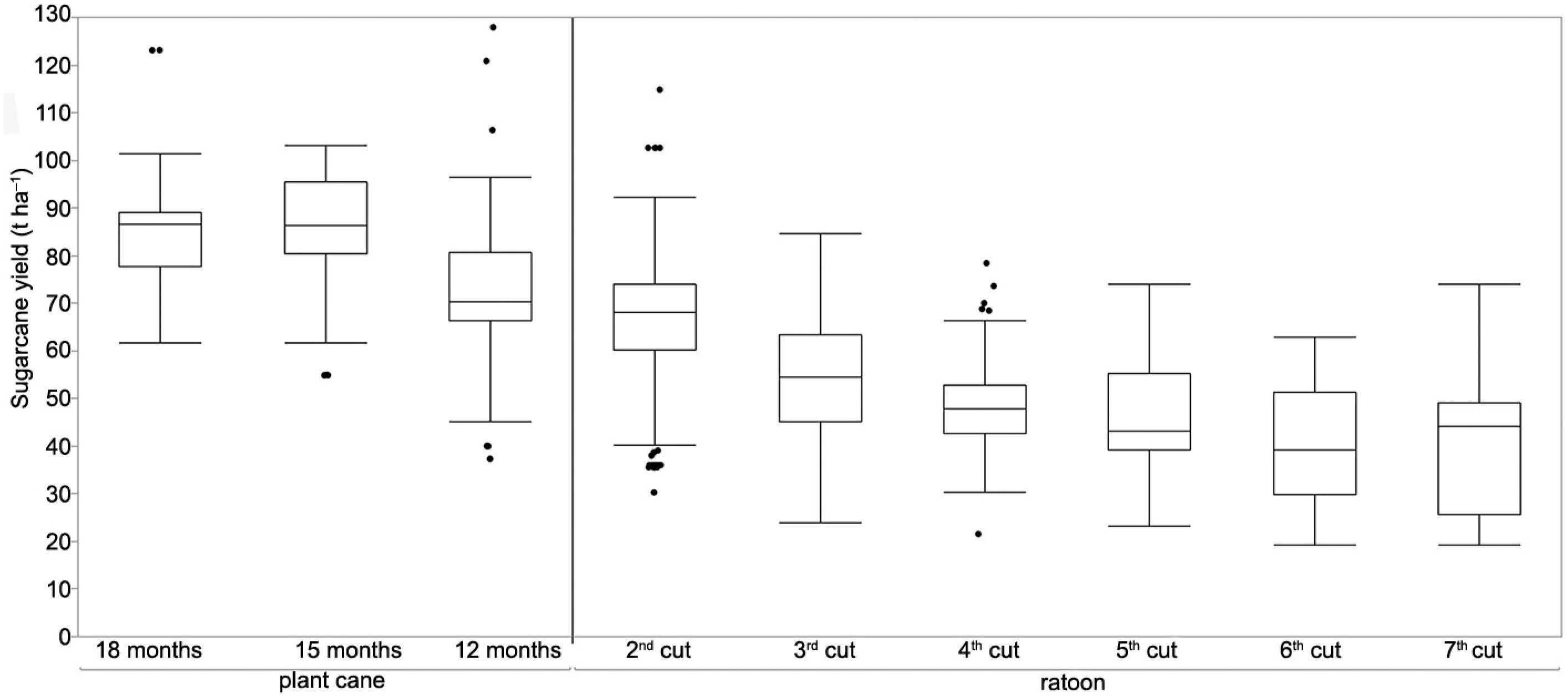
As found by Portier and Anderson (1995), Anderson et al. (1999), Bruggemann et al. (2001), and Ferraro et al. (2009), the number of cuts is the factor of greatest influence on cane yield. With the increase in the number of cuts, there is a decline in average yield, with the 15- and 18-month-old plant canes having the highest yields, followed by 12-month-old plants and finally ratoon canes, in descending order (Figure 3). The impact of intensive mechanization on soil structure, further limiting the development of the roots (Braunack and McGarry, 2006), can be related to the reduction in yield for the sugarcane ratoons. Smith et al. (2005) attribute this reduction in yield to the increased ratio of root/shoot dry mass to age. Simultaneously, these roots have a decreasing ability to absorb nutrients and water. As a result of this phenomenon, reserves that could be aimed at the leaf and stalk are directed to roots with ever-decreasing efficiency as they age.

Figure 3
Box-plot for sugarcane yield: plant cane (18, 15 and 12 months) and ratoon (2^nd harvest onwards).

In the model obtained with the decision tree, there is an interaction between this reduction in average yield as a function of the number of cuts and clay content in the topsoil (0-25 cm). For clay levels above 24 % (N5), the average yield has a slower decrease (slopes with a 95 % Confidence Interval = −5.62 to −4.27) when compared to clay contents below 24 % (N7) (slope with a 95 % Confidence Interval = −7.70 to −7.09), which contributes to significantly higher stabilization of the more clayey condition in relation to the less clayey condition (Figure 4). This phenomenon can be credited to the higher clay content, which is associated with increased water retention and the consequent availability to the plant, which contributes to further development of the aerial part and reduces the death of the roots during drought (Smith et al., 2005). In sandy soils that have lower water availability, the root system is larger and tends to be deeper than in clay soil conditions (Laclau and Laclau, 2009; Smith et al., 2005), leading to a higher root mass that must be restored during every period of drought. In conditions of sugarcane under irrigation, it is often observed that more ratoons can be harvested (Marin et al., 2011).

Figure 4
Influence of clay content in the topsoil (0-25 cm) on sugarcane yield for different number of cuts according to the threshold obtained by the decision tree model.

For the first cut (15 or 18 months), there is an interaction with the calcium content, whereas for the second cut, the interaction is with the Ca/Mg ratio. In both cases, the optimum cut point found by the decision tree is similar to the ones previously obtained by other authors through specific experiments. According to Cantarella et al. (1998), Ca contents higher than 7 mmol_c dm⁻³ did not increase the yield substantially (low correlation between yield and Ca content) when the crop reached a plateau close to 90 % of the potential yield. This is the same limit that was determined by the decision tree as the optimal cut point.

For the Ca/Mg ratio, the decision tree determined 2.67 as the optimal value, whereas Cantarella et al. (1998) found a value of 3.0. In both cases, that is, Cantarella et al.'s (1998) model and our model, higher values for the Ca/Mg ratio resulted in a decrease in yield. The same chemical interaction of the soil with yield is not observed when the first cut is made at 12 months. This can be explained by the management of Ca input – applied through gypsum and lime during soil preparation, usually in the driest months – and the amount of rain associated with sandy soils, which distributes Ca to deeper soil layers up to planting time. The Ca content in the topsoil is different according to the timing of the planting of the first crop.

Since 12-month cane is planted after the first significant rains and 15- and 18-month cane is planted after the highest rainfall period of the year, and the rate of gypsum and lime may not be similar among planting timings (information not available in the database), the Ca content in the topsoil for 15- and 18-month-old plants is significantly lower than that for 12-month-old plants (on average 9.47 and 15.6 mmol_c dm⁻³, respectively). Thus, for 12-month-old plants, the number of blocks in which Ca content was lower than 7 mmol_c dm⁻³ was small; therefore, Ca content in the topsoil is not an influencing factor in this condition. In the second cut, for the less favorable conditions of development (Ca/Mg ≥ 2.67), potassium levels below 1.5 mmol_c dm⁻³ further reduced the yield of sugarcane, which is the value found by the decision tree algorithm. Cantarella et al. (1998) found that values of K below 1.6 mmol_c dm⁻³ significantly reduce the yield (high correlation between yield and K content).

The relationship between Ca, Mg, and K, found in both the plant and the soil, is a factor that greatly influences the crop yield, including sugarcane, because of the competition for the adsorption, absorption, and transport sites at the root surface. Depending on the dynamics of the ionic exchange reactions in soils, an excess of one cation can impair the absorption of another (Marschner, 1995). Although the Ca content and the Ca/Mg ratio did not appear in the decision tree from the third cut onwards, this does not necessarily mean that they did not influence yield, but rather that other factors had greater importance. Another important consideration is that, from the third cut onwards, the levels of nutrients in the subsurface (information not available in the database) have the greatest influence on yield (Landell et al., 2003).

From a practical point of view, these nodes may be interpreted as actionable patterns for increasing yield. If Ca is a limiting factor for the areas in leaf L2 (about 700 ha yr⁻¹), it is possible to estimate a gap of 5,000 tons of sugarcane in node N1 due to this nutrient deficiency. This gap is a consequence of different production in areas under conditions described in L1 in relation to the areas under conditions described in L2. A similar estimation could be made for adjusting the calcium/magnesium relation in nodes N3 and N4 (approximately 3,200 ha yr⁻¹), resulting in a gap of 20,000 tons of sugarcane. This suggests that an increase of 25,000 tons of sugarcane can be achieved through improvements in lime-application protocols, representing an improvement of 2 % compared to the yearly current total production level. Since, for each split, the algorithm chooses the immediate most relevant factor for split, the soil conditions in those areas should be better investigated to diagnose which factors limit production. This would prevent unsuccessful interventions if the factors presented by the model are not the only limitation.

Another point to be considered in the difference between factors of influence on the 12-, 15-, and 18- month-old plant canes and the first ratoon is that the 12-month-old plant cane is more sensitive to less favorable climatic conditions during the cold and dry period than the others. Since a 12-month plant cane is planted at the beginning of the rainy season, the plant reaches the grand growth phase during winter, when temperature and water can limit growth. The dry matter accumulation of sugarcane shows a sigmoid behavior, accumulating approximately 75 % of all dry matter in development phase III, grand growth, which is most susceptible to water restriction (Binbol et al., 2006; Inman-Bamber, 2004; Inman-Bamber and Smith, 2005; Smit and Singels, 2006) and temperature restriction (Inman-Bamber, 1994; Sinclair et al., 2004; Singels et al., 2005). It would seem that considering the region under study has a good distribution of rainfall and that sugarcane has the ability to compensate for less severe water restrictions (Wiedenfeld, 2000), temperature becomes the primary climate factor which determines yield.

The temperature in the grand growth stage also proved to be a factor of influence on yield for the third to the fifth cut ratoon cane in soils with clay contents below 24 % as well as for the 12-month-old plant cane. The cut-off points of the average minimum temperature attribute, whose importance for yield is also highlighted by Binbol et al. (2006), were 15.6 °C for 12-month-old plant canes and 19.6 °C for ratoon canes from the third to the fifth cut under conditions of little clayey surface horizon. These different thresholds may be related to the base temperature for stalk elongation (Inman-Bamber, 1994; Marin et al., 2011) frequently reported close to 16 °C or the base temperature for leaf appearance (Liu et al., 1998) close to 20 °C.

For the ratoon canes ranging from the third to the fifth cut in soils with low clay but less thermal constraint (average minimum temperature in period III > 19.6 °C), there was a positive response to the applied nitrogen doses above 70 kg N ha⁻¹ applied. Sugarcane response to N fertilizer is more often found in cane ratoons than plant canes (e.g. Franco et al., 2010), which is the pattern found by the tree. While this is not surprising, there was an interaction with temperature, where higher doses and minimum temperatures in excess of 19.6 °C in period III resulted in higher yields. This might suggest that for conditions with increased temperature, the availability of nitrogen is a limiting factor.

Even though sugarcane can recover from slightly adverse conditions for growth when conditions improve, limitations prevailing in the rapid growth stage were found to affect yield more than the number of cuts. For areas with more than three harvests (N6), most of the splits were based on factors related to soil or weather. Under low clay content (N7), for areas with three to five harvests (N8), average minimum temperature during the rapid growth stage was the selected factor (splits after N8), while for areas with six or seven harvests (N12), the average precipitation during the rapid growth stage was the determinant factor for yield. As mentioned earlier, the rapid growth stage is more sensitive to boundary conditions of temperature and water availability for change in yield. The temperature in this stage of development proved to be the first factor selected; however, for lower water availability conditions, precipitation was selected in sequence by the tree. The situations of lower water availability can be identified as soils with low clay content or ratoon cane, in which the root system has a lower water absorption capacity.

From an actionability perspective, even though nodes N5, N10, and N12 are not directly actionable as they are environment-related, it is possible to choose more robust varieties in areas with lower clay content or areas that will have most of the growing phase during winter (low precipitation and temperature). Despite not being the best predictive model, the hierarchical structure of the decision tree revealed the relative importance of the predictor variables to sugarcane yield. This hierarchical structure of the decision tree showed different patterns of yield response in relation to interactions with the management and environmental variables. These observed patterns refer to previously researched aspects of sugarcane production.

Even though the patterns found had already been described by previous research, the technique consistently identified a portion of blocks affected by different conditions. If one would try to relate all known factors and test for each factor for all blocks, this could become an unfeasible exercise given the scale of the data. Acting upon the patterns when possible can lead to improvements in yield, leveraging the data already collected by the mill.

In the case of factors relating to management, the current result improves on previous research on the application of decision trees to production databases seeking to understand the effects of different factors on crop yield. Ferraro et al. (2009) found that farm membership was one of the main factors affecting yield. In their case, soil and management data were not available, being summarized by farm membership. Our results show that the decision tree was able to find the specific factors among soil information (e.g. N5 and N7 for clay, and L13 and L14 for sand), soil and management interaction (e.g. L1 and L2 for Ca, and L5 and N4 for Ca/Mg rate), and for the purpose of management (L10 and L11 for N fertilizer).

The tree's results are not meant to establish cause-and-effect relationships, and further investigation and experimentation should be carried out to evaluate them. However, such trees could be an effective tool for prioritizing which interventions to look for in different areas. While the exact results are specific to this data set, a similar structure of results should be expected in data sets from other years, mills, or even different crops.

Conclusion

Analysis of the database through the decision tree technique could describe comprehensible patterns related to yield, even when handling a complex database with a high degree of detail. Part of the patterns identified is actionable and can lead to increases in yield. This work highlights the potential of the decision tree as a tool to assist production system management with actual data from production. This analysis could be carried out systematically in the mill and could be adopted by different mills or even in the production of other crops. It could also be useful for the formulation of hypotheses for specific scientific experiments, particularly for expansion areas, about which knowledge of the production system is still limited. The hierarchy and interactions between factors, which were previously studied in isolation in the literature, have been described, demonstrating that the method is able to consistently reproduce the results previously presented in the literature (experts’ knowledge) and may serve as a basis for the decision-making process or the formulation of hypotheses for specific scientific experiments.

Acknowledgments

The authors thank the Programa FAPESP de Pesquisa em Bioenergia (BIOEN/FAPESP) and Odebrecht Agroindustrial for the financial support from grant #2012/50049-3, Fundação de Amparo à Pesquisa do Estado de São Paulo (FAPESP). The authors also thank the professionals who were interviewed and contributed so that this study could be carried out.

References

• Anderson, D.L.; Portier, K.M.; Obreza, T.A.; Collins, M.E.; Pitts, D.J. 1999. Tree regression analysis to determine effects of soil variability on sugarcane yields. Soil Science Society of America Journal 63: 592-600.
• Binbol, N.; Adebayo, A.; Kwon-Ndung, E. 2006. Influence of climatic factors on the growth and yield of sugar cane at Numan, Nigeria. Climate Research 32: 247-252.
• Braunack, M.V.; McGarry, D. 2006. Traffic control and tillage strategies for harvesting and planting of sugarcane (Saccharum officinarum) in Australia. Soil & Tillage Research 89: 86-102.
• Bruggemann, E.A.; Klug, J.R.; Greenfield, P.L.; Dicks, H.M. 2001. Empirical modeling and prediction of sugarcane yields from field records. Proceedings of South Africa Sugarcane Technologists Association 75: 204-210.
• Cantarella, H.; van Raij, B.; Quaggio, J.A. 1998. Soil and plant analyses for lime and fertilizer recommendations in Brazil. Communications in Soil Science and Plant Analysis 29: 1691-1706.
• De'ath, G.; Fabricius, K.E. 2000. Classification and regression trees: a powerful yet simple technique for ecological data analysis. Ecology 81: 3178-3192.
• Ellis, R.N.; Basford, K.E.; Cooper, M.; Leslie, J.K.; Byth, D.E. 2001. A methodology for analysis of sugarcane productivity trends. I. Analysis across districts. Australian Journal of Agricultural Research 52: 1001-1009.
• Ferraro, D.O.; Ghersa, C.M.; Rivero, D.E. 2012. Weed vegetation of sugarcane cropping systems of northern Argentina: data-mining methods for assessing the environmental and management effects on species composition. Weed Science 60: 27-33.
• Ferraro, D.O.; Rivero, D.E.; Ghersa, C.M. 2009. An analysis of the factors that influence sugarcane yield in northern Argentina using classification and regression trees. Field Crops Research 112: 149-157.
• Franco, H.C.J.; Trivelin, P.C.O.; Faroni, C.E.; Vitti, A.C.; Otto, R. 2010. Stalk yield and technological attributes of planted cane as related to nitrogen fertilization. Scientia Agricola 67: 579-590.
• Hastie, T.; Tibshirani, R.; Friedman, J. 2009. The Elements of Statistical Learning. Springer, New York, NY, USA.
• Inman-Bamber, N.G. 1994. Temperature and seasonal effects on canopy development and light interception of sugarcane. Field Crops Research 36: 41-51.
• Inman-Bamber, N.G. 2004. Sugarcane water stress criteria for irrigation and drying off. Field Crops Research 89: 107-122.
• Inman-Bamber, N.G.; Smith, D.M. 2005. Water relations in sugarcane and response to water deficits. Field Crops Research 92: 185-202.
• Laclau, P.; Laclau, J.-P. 2009. Growth of the whole root system for a plant crop of sugarcane under rainfed and irrigated environments in Brazil. Field Crops Research 114: 351-360.
• Landell, M.G.A.; Prado, H.; Vasconcelos, A.C.M.; Perecin, D.; Rossetto, R.; Bidoia, M.A.P.; Silva, M.A.; Xavier, M.A. 2003. Oxisol subsurface chemical attributes related to sugarcane productivity. Scientia Agricola 60: 741-745.
• Lawes, R.A.; Lawn, R.J.J. 2005. Applications of industry information in sugarcane production systems. Field Crops Research 92: 353-363.
• Lawes, R.A.; McDonald, L.M.; Wegener, M.K.; Basford, K.E.; Lawn, R.J. 2002. Factors affecting cane yield and commercial cane sugar in the Tully district. Australian Journal of Experimental Agriculture 42: 473-480.
• Liu, D.L.; Kingston, G.; Bull, T.A. 1998. A new technique for determining the thermal parameters of phenological development in sugarcane, including sub-optimum and supra-optimum temperature regimes. Agricultural and Forest Meteorology 90: 119-139.
• Marin, F.R.; Jones, J.W.; Royce, F.; Suguitani, C.; Donzeli, J.L.; Palone Filho, W.J.; Nassif, D.S.P. 2011. Parameterization and evaluation of predictions of DSSAT/CANEGRO for brazilian sugarcane. Agronomy Journal 103: 304-315.
• Marschner, H. 1995. Mineral Nutrition of Higher Plants. Academic Press, London, UK.
• Portier, K.M.; Anderson, D.L. 1995. Using Tree Regression to Identify Nutritional and Environmental Factors Affecting Sugarcane Production: Applied Statistics in Agriculture. New Prairie Press, Manhattan, KS, USA.
• Ramburan, S.; Zhou, M.; Labuschagne, M. 2011. Interpretation of genotype × environment interactions of sugarcane: identifying significant environmental factors. Field Crops Research 124: 392-399.
• Sinclair, T.; Gilbert, R.; Perdomo, R.; Shine, J.; Powell, G.; Montes, G. 2004. Sugarcane leaf area development under field conditions in Florida, USA. Field Crops Research 88: 171-178.
• Singels, A.; Smit, M.A.; Redshaw, K.A.; Donaldson, R.A. 2005. The effect of crop start date, crop class and cultivar on sugarcane canopy development and radiation interception. Field Crops Research 92: 249-260.
• Smit, M.A.; Singels, A. 2006. The response of sugarcane canopy development to water stress. Field Crops Research 98: 91-97.
• Smith, D.M.; Inman-Bamber, N.G.; Thorburn, P.J. 2005. Growth and function of the sugarcane root system. Field Crops Research 92: 169-183.
• Wiedenfeld, R.P. 2000. Water stress during different sugarcane growth periods on yield and response to N fertilization. Agricultural Water Management 43: 173-182.
• Zhang, B.; Valentine, I.; Kemp, P. 2005. Modelling the productivity of naturalised pasture in the North Island, New Zealand: a decision tree approach. Ecological Modelling 186: 299-311.
• Zhang, B.; Valentine, I.; Kemp, P.; Lambert, G. 2006. Predictive modelling of hill-pasture productivity: integration of a decision tree and a geographical information system. Agricultural Systems 87: 1-17.
• Zheng, H.; Chen, L.; Han, X.; Zhao, X.; Ma, Y. 2009. Classification and regression tree (CART) for analysis of soybean yield variability among fields in northeast China: the importance of phosphorus application rates under drought conditions. Agriculture, Ecosystems and Environment 132: 98-105.

Appendix 1 Description of the predictor attributes.

No. Code Description No. Code Description 1 Al Alumum content in the soil in the 0-25 cm layer 35 Mg Magnesium content in the soil in the 0-25 cm layer 2 Sand1 Percentage of sand in the soil in the 0-25 cm layer 36 MgK Mg/K ratio in the soil in the 0-25 cm layer 3 Sand2 Percentage of sand in the soil in the 25-50 cm layer 37 OM Organic matter content in the soil in the 0-25 cm layer 4 Sand3 Percentage of sand in the soil in the 80-100 cm layer 38 P Phosphorus content in the soil in the 0-25 cm layer 5 Clay1 Percentage of clay in the soil in the 0-25 cm layer 39 pH pH in the soil in the 0-25 cm layer 6 Clay2 Percentage of clay in the soil in the 25-50 cm layer 40 avg.ppt.I Average daily precipitation in phase I (sprouting) 7 Clay3 Percentage of clay in the soil in the 80-100 cm layer 41 avg.ppt.II Average daily precipitation in phase II (tillering) 8 Ca Calcium content in the soil in the 0-25 cm layer 42 avg.ppt.III Average daily precipitation in phase III (growth) 9 CaK Ca/K ratio in the soil in the 0-25 cm layer 43 avg.ppt.IV Average daily precipitation in phase IV (ripening) 10 CaMg Ca/Mg ratio in the soil in the 0-25 cm layer 44 accum.ppt.I Accumulated precipitation in phase I (sprouting) 11 CycleD Cycle duration in days 45 accum.ppt.II Accumulated precipitation in phase II (tillering) 12 Cut Number of cuts 46 accum.ppt.III Accumulated precipitation in phase III (growth) 13 CEC CEC in the soil in the 0-25 cm layer 47 accum.ppt.IV Accumulated precipitation in phase IV (ripening) 14 Dens Soil density 48 Sb Sum of bases in the soil in the 0-25 cm layer 15 CutTime Cutting time (fall, winter, spring) 49 avg.maxt.I Average maximum temperature in phase I (sprouting) 16 Drought.I Higher number of consecutive days without precipitation in phase I (sprouting) 50 avg.maxt.II Average maximum temperature in phase II (tillering) 17 Drought.II Higher number of days without precipitation in phase II (tillering) 51 avg.maxt.III Average maximum temperature in phase III (growth) 18 Drought.III Higher number of consecutive days without precipitation in phase III (growth) 52 avg.maxt.IV Average maximum temperature in phase IV (ripening) 19 Drought.IV Higher number of consecutive days without precipitation in phase IV (repining) 53 avg.avgt.I Average temperature in phase I (sprouting) 20 sourceK Source of fertilization with potassium (fertilizer/vinasse) 54 avg.avgt.II Average temperature in phase II (tillering) 21 ADD.I Accumulated degree days in phase I (sprouting) 55 avg.avgt.III Average temperature in phase III (growth) 22 ADD.II Accumulated degree days in phase II (tillering) 56 avg.avgt.IV Average temperature in phase IV (ripening) 23 ADD.III Accumulated degree days in phase III (growth) 57 avg.mint.I Average minimum temperature in phase I (sprouting) 24 Frost Occurrence of frost 58 avg.mint.II Average minimum temperature in phase II (tillering) 25 GradText (Percentage clay 25-50 cm/ Percentage clay 0-25 cm) 59 avg.mint.III Average minimum temperature in phase III (growth) 26 HAl H+Al content in the soil in the 0-25 cm layer 60 avg.mint.IV Average minimum temperature in phase IV (ripening) 27 Kinput kg ha−1 of fertilization with potassium 61 Cake Amount of filter cake applied 28 Moinput kg ha−1 of fertilization with molybdenum 62 V Percent of base saturation in the soil in the 0-25 cm layer 29 Ninput kg ha−1 of fertilization with nitrogen 63 Variety Variety cultivated 30 Pinput kg ha−1 of fertilization with phosphorus 64 DrySpell.I Number of periods longer than or equal to 10 days without rain in phase I (sprouting) 31 K Potassium content in the soil in the 0-25 cm layer 65 DrySpell.II Number of periods longer than or equal to 10 days without rain in phase II (tillering) 32 KCaMg K/(Ca + Mg)½ ratio in the soil in the 0-25 cm layer 66 DrySpell.III Number of periods longer than or equal to 10 days without rain in phase III (growth) 33 KCEC K/CEC ratio in the soil in the 0-25 cm layer 67 DrySpell.IV Number of periods longer than or equal to 10 days without rain in phase IV (ripening) 34 M Soil saturation by aluminum (m%) in the 0-25 cm layer 68 Vinasse Volume of vinasse applied

No.	Code	Description	No.	Code	Description
1	Al	Alumum content in the soil in the 0-25 cm layer	35	Mg	Magnesium content in the soil in the 0-25 cm layer
2	Sand1	Percentage of sand in the soil in the 0-25 cm layer	36	MgK	Mg/K ratio in the soil in the 0-25 cm layer
3	Sand2	Percentage of sand in the soil in the 25-50 cm layer	37	OM	Organic matter content in the soil in the 0-25 cm layer
4	Sand3	Percentage of sand in the soil in the 80-100 cm layer	38	P	Phosphorus content in the soil in the 0-25 cm layer
5	Clay1	Percentage of clay in the soil in the 0-25 cm layer	39	pH	pH in the soil in the 0-25 cm layer
6	Clay2	Percentage of clay in the soil in the 25-50 cm layer	40	avg.ppt.I	Average daily precipitation in phase I (sprouting)
7	Clay3	Percentage of clay in the soil in the 80-100 cm layer	41	avg.ppt.II	Average daily precipitation in phase II (tillering)
8	Ca	Calcium content in the soil in the 0-25 cm layer	42	avg.ppt.III	Average daily precipitation in phase III (growth)
9	CaK	Ca/K ratio in the soil in the 0-25 cm layer	43	avg.ppt.IV	Average daily precipitation in phase IV (ripening)
10	CaMg	Ca/Mg ratio in the soil in the 0-25 cm layer	44	accum.ppt.I	Accumulated precipitation in phase I (sprouting)
11	CycleD	Cycle duration in days	45	accum.ppt.II	Accumulated precipitation in phase II (tillering)
12	Cut	Number of cuts	46	accum.ppt.III	Accumulated precipitation in phase III (growth)
13	CEC	CEC in the soil in the 0-25 cm layer	47	accum.ppt.IV	Accumulated precipitation in phase IV (ripening)
14	Dens	Soil density	48	Sb	Sum of bases in the soil in the 0-25 cm layer
15	CutTime	Cutting time (fall, winter, spring)	49	avg.maxt.I	Average maximum temperature in phase I (sprouting)
16	Drought.I	Higher number of consecutive days without precipitation in phase I (sprouting)	50	avg.maxt.II	Average maximum temperature in phase II (tillering)
17	Drought.II	Higher number of days without precipitation in phase II (tillering)	51	avg.maxt.III	Average maximum temperature in phase III (growth)
18	Drought.III	Higher number of consecutive days without precipitation in phase III (growth)	52	avg.maxt.IV	Average maximum temperature in phase IV (ripening)
19	Drought.IV	Higher number of consecutive days without precipitation in phase IV (repining)	53	avg.avgt.I	Average temperature in phase I (sprouting)
20	sourceK	Source of fertilization with potassium (fertilizer/vinasse)	54	avg.avgt.II	Average temperature in phase II (tillering)
21	ADD.I	Accumulated degree days in phase I (sprouting)	55	avg.avgt.III	Average temperature in phase III (growth)
22	ADD.II	Accumulated degree days in phase II (tillering)	56	avg.avgt.IV	Average temperature in phase IV (ripening)
23	ADD.III	Accumulated degree days in phase III (growth)	57	avg.mint.I	Average minimum temperature in phase I (sprouting)
24	Frost	Occurrence of frost	58	avg.mint.II	Average minimum temperature in phase II (tillering)
25	GradText	(Percentage clay 25-50 cm/ Percentage clay 0-25 cm)	59	avg.mint.III	Average minimum temperature in phase III (growth)
26	HAl	H+Al content in the soil in the 0-25 cm layer	60	avg.mint.IV	Average minimum temperature in phase IV (ripening)
27	Kinput	kg ha−1 of fertilization with potassium	61	Cake	Amount of filter cake applied
28	Moinput	kg ha−1 of fertilization with molybdenum	62	V	Percent of base saturation in the soil in the 0-25 cm layer
29	Ninput	kg ha−1 of fertilization with nitrogen	63	Variety	Variety cultivated
30	Pinput	kg ha−1 of fertilization with phosphorus	64	DrySpell.I	Number of periods longer than or equal to 10 days without rain in phase I (sprouting)
31	K	Potassium content in the soil in the 0-25 cm layer	65	DrySpell.II	Number of periods longer than or equal to 10 days without rain in phase II (tillering)
32	KCaMg	K/(Ca + Mg)½ ratio in the soil in the 0-25 cm layer	66	DrySpell.III	Number of periods longer than or equal to 10 days without rain in phase III (growth)
33	KCEC	K/CEC ratio in the soil in the 0-25 cm layer	67	DrySpell.IV	Number of periods longer than or equal to 10 days without rain in phase IV (ripening)
34	M	Soil saturation by aluminum (m%) in the 0-25 cm layer	68	Vinasse	Volume of vinasse applied

Edited by

Edited by: Gerrit Hoogenboom

Publication Dates

• Publication in this collection
  Jul-Aug 2019

History

• Received
  12 July 2017
• Accepted
  04 Apr 2018