Numerical study of upstream disturbances on the performance of electromagnetic and ultrasonic flowmeters

ABSTRACT

Electromagnetic and ultrasonic flowmeters are high precision devices that can measure the water flow in pressurized irrigation networks. In these networks, the inadequate installation distance of flow control valves generates upstream disturbances which will increase measurement errors and reduce the accuracy of the equipment. Therefore, estimating these errors is important to establishing the correct installation distance of the hydraulic accessories and to ensuring the metrological reliability of the flowmeters. This work proposes a numerical study using Computational Fluid Dynamics to evaluate water flow behavior in pipes and estimate measurement errors caused by gate and butterfly valves in installation configurations found at pressurized irrigation networks. The numerical simulations were made for gate (15, 50 and 75 % closed) and butterfly (open and 30º closed) valves installed three and six diameters (3D and 6D) from the flowmeters. The numerical study with three-dimensional simulation allows for evaluating the flow behavior and estimating measurement errors correctly. According to the study, the installation configurations of the gate and butterfly valves change the flow velocity profile at different positions in the pipe, generating both positive and negative measurement errors at both flowmeters. Among the tested configurations, only the butterfly valve installed 3D and 6D from the electromagnetic flowmeter ensured the measurement accuracy required by ISO 4064.

CFD; pressurized irrigation; water flowmeter; water supply network

Introduction

At the present time, technologically advanced electromagnetic (EM) and ultrasonic (US) flowmeters are used to accurately meter liquid flows. They present certain advantages ( Zhang et al., 2014 ; Zheng et al., 2015 ), which can be exploited in diverse areas ( Baker, 2011 ; Shi et al., 2015 ), including rural irrigation and water systems ( Shang, 2017 ; Massey et al., 2017 ; Massuel et al., 2017 ).

Commonly, microirrigation control head includes valving, water filters, pumps, injectors, controllers and the monitoring equipment required to deliver and control water in irrigation networks. On occasion, flowmeters are found inside the control head systems in improper configurations. Maintaining appropriate distances between various components to ensure reliable functioning of meters and gauges and facilitating operation, maintenance, and cleaning of filters is often difficult due to an incorrect structural design of the system control head ( Figure 1A, B, C, D ).

Figure 1
– EM flowmeter installed in a microirrigation control head with an elbow and a by-pass upstream (A); Woltman meter mounted beside an elbow and a butterfly valve upstream. The picture shows the wrong design of this control head system without appropriate distances (B); upstream section with an automatic butterfly valve (C) and US flowmeter installed downstream of that valve (D).

EM and US flowmeters estimate the circulating flow from the water velocity inside the pipe. Knowledge of their behavior is essential for precise measuring, especially in the presence of flow-disturbing hydraulic elements. Since each of these elements can affect flow in a different way ( Sapra et al., 2011 ), it is recommended to determine the safe installation distance of flowmeters, which is normally determined by means of an experimental analysis and/or numerical simulations ( Bates, 2000 ; Dong-Keun and Yong, 2012 ; Hilgenstock and Ernst, 1996 ).

Computational Fluid Dynamics (CFD) is a numerical technique used for solving complex problems in modern engineering practice ( Tu et al., 2018 ). Studies in this field have validated the use of the CFD technique in simulating accessories and/or analysis of flow behavior ( Manzano et al., 2016 ; Silva et al., 2016 ), including the above-mentioned devices ( Holm et al., 1995 ; Chen et al., 2015 ; Weissenbrunner et al., 2016 ). Studies related to these flowmeters estimate metering precision with different types of accessories installed in different positions, degrees of closure and distances from the meter, etc. ( Stoker et al., 2012 ; Wada et al., 2012 ; Zheng et al., 2013 ).

Since accessories such as gate and butterfly valves are used to control the flow, a few studies have appeared which utilize numerical simulations and computational analysis of both types of flowmeter mostly carried out by experimental tests ( Heritage, 1989 ).

This work proposes a numerical study using CFD techniques to evaluate the water flow behavior and estimate the measurement errors of the EM and US flowmeters caused by gate and butterfly valves in installation configurations found in pressurized irrigation networks.

Materials and Methods

The first step of the numerical analysis involved the analysis of the operating principles of these electronic devices to determine the parameters required in numerical analysis to calculate the circulating flow and the metering error.

The operating principle of the electromagnetic flowmeter is based on Faraday’s Law ( ISO 6817, 1992 ). This principle states that an electromotive force or voltage (E) is induced between the extremes of any fluid conductor that passes through an electromagnetic field. This voltage is proportional to fluid velocity ( V ) along its length ( L ) at the intensity of the magnetic field ( B ) and to the calibration constant ( K ) of the instrument (Equation 1).

$E=KBLV$ (1)

In practice, the electromotive force generated by the water flow is the result of weighting the velocities in the metered cross-section. Using Shercliff’s (1962) weighting function ( W ), the voltage difference between the electrodes (Δ U _EE ) of the flowmeter can be calculated (Equation 2) as follows:

$\mathrm{\Delta }{U}_{EE}=\int {\int }_{MS}\overrightarrow{W}\to \left(r,\theta \right)\overrightarrow{B}\left(\theta \right)\overrightarrow{V}\left(r,\theta \right)drd\theta$ (2)

in which MS is the measurement pipe cross section; r the line where the point of the metering cross-section is located; and θ the angle whose origin is parallel to the direction of the intensity of the magnetic flow.

The circulating flow ( Q ) can be calculated by the following Equation 3, which, in polar coordinates, depends on the area of measurement ( a ) and on r and θ ( Baker, 2000 ):

$Q=\int {\int }_{MS}\frac{a^4+a^2{r}^2\cos 2\theta }{a^4+2a^2{r}^2\cos 2\theta +r^4}{V}_x\left(r,\theta \right)rdrd\theta$ (3)

On the other hand, the operating principle of the time-transit ultrasonic flowmeter is based on the variation of the absolute propagation speed of sound between two transducers acting as emitter and receiver of a series of sound waves Arregui et al. (2007 .

From the position of the transducers and the diameter of the pipeline the difference in transit time (Δ t ) of the sound waves can be calculated by Equations 4 and 5, as identified in Arregui et al. (2007) .

$t_1=\frac{L}{c+V\cos \alpha }{t}_2=\frac{L}{c-V\cos \alpha }$ (4)

$t_1-t_2=\Delta t\frac{2LV\cos \alpha }{c^2+V^2{\cos }^2\alpha }$ (5)

in which t ₁ is the elapsed time from emitter to receiver; t ₂ the elapsed time from receiver to emitter; L the distance between transducers; c the propagation speed of sound in the water, which is equal to 1,482 m s¹; for water at 20 ºC; V the mean velocity of the fluid in the pipe; and α the angle between the axis of the pipe and the fictional line of sound waves.

Considering that c ² is definitely greater than V ² cos ²α, the latter can be omitted, so that the fluid velocity ( V ), and the circulating flow ( Q ) can be obtained by Equations 6 and 7 ( Arregui et al., 2007 ).

$V=\frac{\Delta t{c}^2}{2L\cos \alpha }$ (6)

$Q=AV=\frac{\pi D^2}{4}\frac{\Delta t{c}^2}{2L\cos \alpha }$ (7)

It should be remembered that the mean velocity obtained from the path of the sound wave ( V ) is not exactly the mean fluid velocity throughout the whole cross-section (V), but both velocities are related by a proportional factor ( k ) estimated from the Reynold’s number ( Re ) (Equations 8 and 9):

$\overline{V}=\mathcal{k}V$ (8)

$\mathcal{k}=\frac{1}{1.12-0.011LogRe}$ (9)

The second step in the study was the numerical simulation, from which the velocity profiles were obtained at different points in the cross-section, which provided information on how the water flow in a pipe can be altered by the installation of hydraulic accessories.

Simulations were carried out using the Fluent^© 6.1 software package divided into three phases: pre-processing, processing and post-processing.

In the first phase, the Gambit^© graphic interface was used to define the detailed geometry in 3D of the components and the grid of the computational domain ( Figure 2A, B, C ). This was obtained by defining the flowmeters and hydraulic accessories from drawings of the desired configurations and by generating the grid and its refinement. Before the processing phase, the fluid properties and the boundary conditions adopted in each case were established. Inlet velocity and pressure at outlet were the boundary conditions chosen for the inlet and outlet pipe flow characteristics, respectively. ( Table 1 ).

Figure 2
– Computational domain for gate valve simulations (A) and for butterfly valve simulations (B); detail of the grid used in gate valve simulations (C).

Table 1
– Summary of cases studied and boundary conditions for electromagnetic and transit-time ultrasonic flowmeters.

Cases simulated
Configuration	Reference	Gate valve1			Butterfly valve2
Degrees open	-	75 %, 50 %, 25 % closed			Open, 30° closed
Distance	-	0D, 3D, 6D			0D, 3D, 6D
Boundary conditions
Inlet velocity (m s–1)	1, 2, 3, 4, 6	1, 2, 3, 4, 6	1, 2, 3, 4, 6	1, 2, 3, 4, 6	1, 2, 3, 4, 6	1, 2, 3, 4, 6
Pressure at outlet (bar)	3	3	3	3	3	3
Condition of wall k (mm)	0.1	0.1	0.1	0.1	0.1	0.1
Wall symmetry	Yes	Yes	Yes	Yes	No	No

• D = pipe diameter; ¹The gate valve closes from top to bottom; ²The butterfly valve closes from right to left.

The devices evaluated were an electromagnetic flowmeter and a time-transit ultrasonic flowmeter. The hydraulic elements consisted of a gate and a butterfly valve, with 80 mm nominal diameter, equal to that of the pipe.

The studied configurations, commonly found in pressurized irrigation networks, were generated for three cases. In the first the flowmeters were fitted to the pipe with no hydraulic accessories (reference case). The gate and butterfly valves were installed on the pipe in the second and third cases, respectively, in which different degrees of closure and distances from the meters were tested.

The grid was generated by discretizing and refining the computational domains described in control volumes of 1 mm asymmetric cells by the Hanging Node technique, which allows for cells to be duplicated to create an optimal non-uniform grid, in this case doubly refined in the zones with high velocity or pressure variations ( Versteeg and Malalasekera, 1995 ). The total number of cells in the grid was 153,542. Refined grids were studied to improve the computational results but no significant enhancement was found.

The cases tested were for turbulent flow with Re number in the range of 80,000 to 480,000 and the boundary conditions of each simulation can be seen in Table 1 .

In the processing phase, the differential equations were discretized into control volumes or cells by the Finite Volumes Method and approximated by the Finite Differences Technique. This method allowed the numerical simulations to be three-dimensional (3D).

The coherent union between fluid pressures and volumes was established by iterative mathematical calculation algorithms of the type Semi-Implicit Method for Pressure-Linked Equations (SIMPLE). The mathematical model and the method of modeling turbulent viscosity were the Reynolds Average Navier-Stokes (RANS) and the Standard k-ε Turbulent Model, respectively. A numerical model near the wall was used with a pipe with absolute roughness of 0.1 mm according to the log law near the wall.

In the post-processing phase the main results of the simulations were organized graphically and used to identify how the water flow reached the flowmeters. Axial velocity profiles were extracted in different lines to simplify subsequent calculations and better fit the velocities in all directions by interpolations in this contour plane.

The final step of the study was performed by numerical solution to allow the simulation of actual situations. For both metering devices, the velocity vectors obtained from the simulations were combined with the corresponding measurement plane or diametral chord obtained by the theoretical equations required to estimate the metering errors at any instrument position ( Error ) (Equation 10).

$Error=\left(\frac{Q_{dist.}-Q_{ref.}}{Q_{ref.}}\right)100$ (10)

in which Q _dist. is the distorted flow and Q _ref. the reference flow.

Figure 3A, B, C, D shows a graphic representation of each simulation of the measuring cross-section of the EM flowmeter and the measuring chords of the US flowmeter.

Figure 3
– Measurement area of the electromagnetic flowmeter (A); number of points extracted from cross-section of a round-electrode electromagnetic flowmeter (B); measurement chords of a plane (C); and projection of a velocity profile on the diametral chord of a transit-time ultrasonic flowmeter (D). α is the angle between the pipe axis and the fictional line of sound waves (30º); L the length between emitter and receiver (160 mm); and D the pipe diameter (80 mm).

The measurement error associated with the electromagnetic flowmeter was estimated by integrating all the surface of the weighted velocity vectors in the measurement cross-section ( Figure 3A ). These velocity vectors are equivalent to the mean velocity of a differential cross-section defined by the number of points extracted from each simulation ( Figure 3B ).

On the other hand, the measurement error associated with the ultrasonic flowmeter was estimated by considering a measurement plane ( Figure 3C ). The decomposition of the velocity vectors in the line between the transducers was projected onto the diametral measurement chord ( Figure 3D ). With these velocities discretized into 98 points along the chord, the variation found in the mean fluid velocity in the transit time between transducers was calculated with an altered profile.

By changing the system of coordinates (Cartesian to Polar) the velocity vectors of the numerical simulations in the above equations were used to estimate the flows and measurement errors of both flowmeters. Although these flowmeters can achieve high precision (errors between 0.2 % and 0.5 %), the acceptable error was assumed equal to ± 2 % ( ISO 4064, 2014 ).

Afterwards, to determine the way in which the flow reached both flowmeters, planes and lines were extracted with the axial velocities in the zones of interest; in the EM meter this was in the cross-section between the electrodes parallel to the magnetic flow intensity, whereas in the ultrasonic flowmeter it was extracted in the fictional chord between both transducers.

Finally, the numerical study using CFD techniques was validated by comparing analytical results with empirical results for the reference case. Simulations showed a high adjustment with errors lower than 2 % within the model and the experimental flow rate, as seen in Table 2 .

Table 2
– Validation of flow numerical simulations with empirical test.

EM flow meter			Ultrasonicflow meter
Ref. Numerical Q (m3 h–1)	Empirical test Q (m3 h–1)	E (%)	Ref. Numerical Q (m3 h–1)	Empirical test Q (m3 h–1)	E (%)
33.25	33.8	-1.63	30.85	31.4	-1.75
66.88	65.9	1.49	61.02	61.3	-0.46
100.34	100.1	0.24	92.33	92.8	-0.51
33.25	33.2	0.15	30.64	31.1	-1.48
66.5	65.9	0.91	61.43	61.5	-0.11
99.78	99.1	0.69	92.3	92.6	-0.32
33.69	33.8	-0.33	30.65	31.2	-1.76
67.47	66.8	1.00	61.5	61.8	-0.49
101.28	101.4	-0.12	92.45	92.6	-0.16
34.25	34.1	0.44	30.5	30.7	-0.65
67.7	67.9	-0.29	61.62	62.0	-0.61
102.82	102.9	-0.08	92.4	92.3	0.11
34.24	33.8	1.30	30.68	30.6	0.26
67.79	67.5	0.43	61.8	62.1	-0.48
102.76	102.4	0.35	92.62	92.5	0.13

• Ref. num = reference numerical case; Empirical Test flow results; Q = circulating flow; E = simulation error.

Flow tests were carried out on an ITA Sustainable Urban Water Management test bench at the Universitat Politècnica de València, Valencia, Spain. The principal elements used on the test bench included: electromagnetic flow meter and a transit-time ultrasonic flow meter with a precision of ± 0.5 % and ± 2.0 – 5.0 % respectively; 0-16 bar range pressure transducer accurate to ± 0.28 %; two 18.5 kW pumps installed in parallel; epoxy coated cast iron pipes of DN (Diameter Nominal) 80 and 100 mm; personal computer, and a data acquisition system with Labview software©.

Results and Discussion

The most interesting results of the CFD simulations show that the largest distortions in the velocity profile occur with the hydraulic elements in their most closed positions and mainly when placed close to both flowmeters ( Figure 4A, B, C ).

Figure 4
– Velocity profiles distorted by hydraulic elements installed upstream at different distances from an electromagnetic and transit-time ultrasonic flowmeter: measurement area of the electromagnetic flowmeter for 75 % closed gate valve (A); 30º closed butterfly valve (B); and evolution of water flow after passing through these valves (75 % and 30º closed, respectively) (C). Flows used were 70 and 100 m3 h–1 for gate and butterfly valves, respectively.

The gate valve generates the highest velocities in the lower section of the pipe ( Figure 4A ), while the butterfly valve does so in a zone on the left of the pipe ( Figure 4B ). This behavior is induced by the short distance between both elements, which does not allow the profile to normalize.

Only when the accessories are at 3D from the flowmeters does the velocity profile show an insignificant effect, and especially so at 6D from the meter. Figure 4C shows the imbalance caused by the 75 % closed gate valve and the open butterfly valve and the distance required for the profile to return to normal.

The numerical results for the electromagnetic flowmeter confirm that the changes in flow velocity caused by the valves increase with the degree of closure and are more marked when the flowmeter is placed at the shortest distance ( Table 3 ).

Table 3
– Measurement errors of electromagnetic flowmeter caused by gate and butterfly valves corresponding to different operating conditions and positions.

Case	Gate valve						Butterfly valve
	75 % closed		50 % closed		25 % closed		Open		30° closed
	Q (m3 h–1)	E (%)	Q (m3 h–1)	E (%)	Q (m3 h–1)	E (%)	Q (m3 h–1)	E (%)	Q (m3 h–1)	E (%)
Ref.	33.25	-	33.25	-	33.69	-	34.25	-	34.24	-
	66.88	-	66.50	-	67.47	-	67.70	-	67.79	-
	100.34	-	99.78	-	101.28	-	102.82	-	102.76	-
0D	31.59	-4.99	33.26	0.02	35.21	4.51	34.37	0.35	35.45	3.53
	62.91	-5.93	66.54	0.06	70.48	4.46	68.10	0.59	69.48	2.49
	94.24	-6.08	99.85	0.08	105.70	4.36	103.22	0.39	106.36	3.50
3D	33.13	-0.36	32.95	-0.90	34.40	3.43	34.22	-0.09	33.64	-1.75
	66.16	-1.08	66.14	-0.54	68.80	3.53	68.46	1.12	67.00	-1.17
	99.26	-1.08	99.31	-0.46	103.30	3.60	102.68	-1.14	100.87	-1.84
6D	33.26	0.03	32.74	-1.53	34.50	3.73	34.14	-0.32	34.20	-0.12
	66.26	-0.92	65.43	-1.61	69.00	3.83	68.11	0.61	67.60	-0.03
	99.48	-0.86	98.20	-1.58	103.50	3.80	102.25	-0.55	102.65	-0.11

• Ref. = reference case (no hydraulic accessories); D = installation distance equivalent to 1 pipe diameter; Q = circulating flow; E = measurement error.

The graph of the gate valve results shows how the distribution of the velocity profile distorted by the degrees of closure and distance from the meter affects the measurement of the flow ( Figure 5A, B ).

Figure 5
– Velocity profile perpendicular to measurement cross-section between electrodes of electromagnetic flowmeter for 75 % closed gate valve at different distances from the meter (A); and with different degrees of closure beside the meter (B).

For example, the closest position beside the meter ( Figure 5A ) generates higher velocities in the lower section of the pipe, which, when weighted by the Shercliff Function, reduce their magnitude and cause negative measurement errors. However, these errors rise less and the velocity profile is more stable when the distance increases from 3D to 6D.

In the less closed position ( Figure 5B ), it can be seen that the velocity profile reaches high values in the central zone of the measurement cross-section, where the Shercliff coefficients are higher, and causes overestimation of the weighted velocity and, thus, of the circulating flow.

This means that when the hydraulic element is close to the flowmeter, reducing the degree of closure reduces the flow imbalance but does not significantly improve the flow measurement accuracy.

The degree of distortion produced by the butterfly valve is in general lower than that of the gate valve, so that measurements are less affected. The valve design does not allow for installation at a distance shorter than 3D from the meter and this helps to stabilize the water flow.

From the graphs extracted by Fluent it can be observed that when the butterfly valve is open its influence on the electromagnetic flowmeter is practically absent, and when closed 30º it causes overestimation errors that diminish with longer straight distances between both elements.

The main conclusions drawn from the simulations concerning the electromagnetic flowmeter reveal that when the flow is distorted at high velocities in zones far from the measuring electrodes, the instrument tends to underestimate. However, when the flow is unbalanced but maintains its symmetry in the cross-section, where the highest velocities are in the center zone or close to the electrodes, the circulating flow is overestimated. This means that keeping a 6D straight pipe distance between the instrument and the disturbing element will significantly reduce the error in all cases.

The numerical results of the US flowmeter, despite being similar to those of the EM flowmeter as regards the influence of the valves, indicate that this device is more sensitive to flow distortions ( Table 4 ).

Table 4
– Measurement errors of transit-time ultrasonic flowmeter caused by gate and butterfly valves corresponding to different operating conditions and position.

Case	Gate valve						Butterfly valve
	75 % closed		50 % closed		25 % closed		Open		30° closed
	Q (m3 h–1)	E (%)	Q (m3 h–1)	E (%)	Q (m3 h–1)	E (%)	Q (m3 h–1)	E (%)	Q (m3 h–1)	E (%)
Ref.	30.85	-	30.64	-	30.65	-	30.5	-	30.68	-
	61.02	-	61.43	-	61.50	-	61.62	-	61.8	-
	92.33	-	92.30	-	92.45	-	92.4	-	92.62	-
0D	36.92	19.68	33.11	8.06	31.54	2.89	33.59	10.13	36.72	19.69
	74.35	21.85	67.09	9.21	62.85	2.20	67.79	10.01	73.77	19.37
	111.95	21.25	101.08	9.51	94.30	2.00	101.06	9.37	112.12	21.05
3D	36.15	17.18	32.21	5.12	30.86	0.69	32.05	5.08	36.14	17.8
	72.51	18.83	64.53	5.05	61.80	0.49	64.8	5.16	71.13	15.09
	109.14	18.21	97.05	5.14	92.81	0.39	95.9	3.79	108.1	16.71
6D	35.96	16.56	32.10	4.77	30.76	0.35	31.59	3.57	35.39	15.35
	71.94	17.90	64.10	4.35	61.33	-0.28	63.73	3.42	69.82	12.98
	108.40	17.40	96.14	4.16	92.80	0.38	95.2	3.03	101.62	9.72

• Ref. = reference case (no hydraulic accessories); D = installation distance equivalent to 1 pipe diameter; Q = circulating flow; E = measurement error.

The figure shows how the distribution of velocities distorted by the gate valve has a more significant effect on flow measurement ( Figure 6A, B, C ).

Figure 6
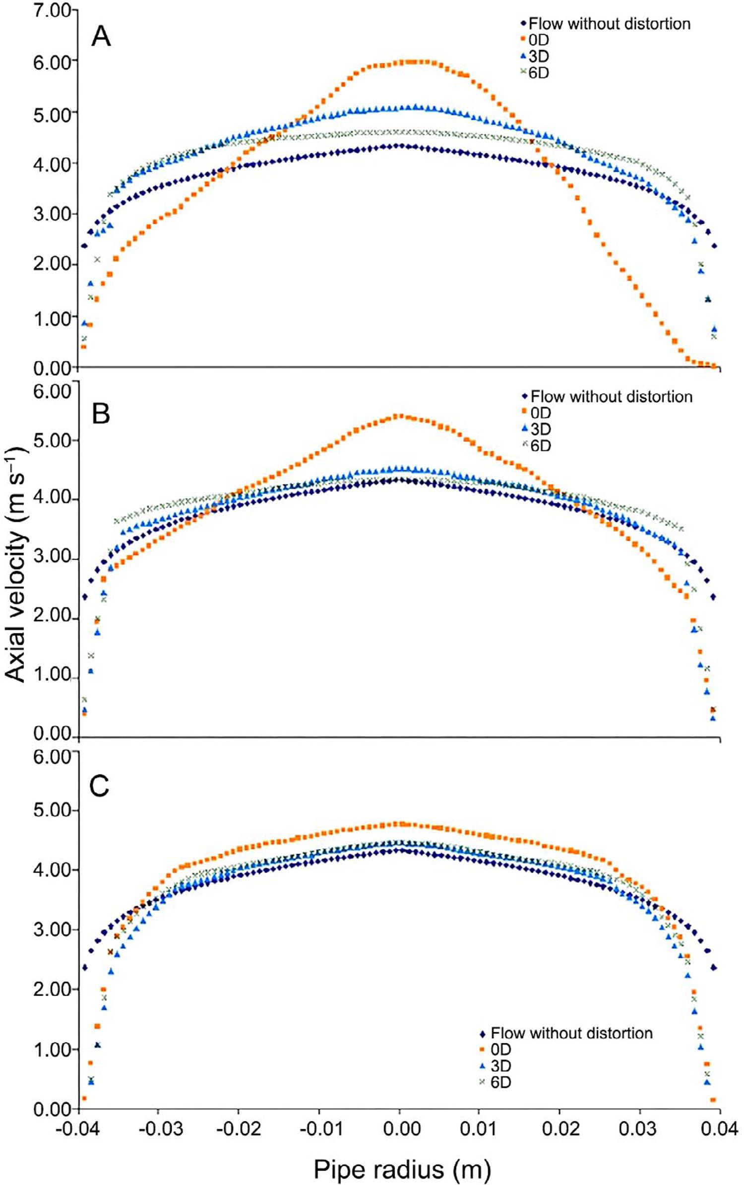
– Velocity profile for 75 % closed gate valve (A); 50 % closed (B); and 25 % closed (C), installed at different distances from an electromagnetic and transit-time ultrasonic flowmeter.

The velocity profile is most distorted in the extreme case, with the valve 75 % closed at 0D ( Figure 6A ). The velocities projected onto the measurement chord, which are high in the central zone of the pipe, validate the overestimation of approximately + 20 %. When the distances were increased from 3D to 6D the measurements improved.

With less-closed valves, the differences in the velocity at the center and near the wall of the pipe are smaller and the measurement errors are reduced. This reduction, with the valve at 0D can reach + 8 % for a closure of 50 % ( Figure 6B ) and up to + 3 % for 25 % ( Figure 6C ). In these cases, the velocities in all the chord are slightly higher in the central zone, which explains the positive measurement errors.

As can be seen from the results, this measuring instrument is highly sensitive to flow distortions ( Furuichi et al., 2009 ), since the estimated flows are much higher than those actually circulating. The safe distance for installing hydraulic accessories should therefore be longer than 6D upstream to avoid overestimation errors.

In experiments with a 25 and 50 % closed gate valve, the measurement errors of transit time ultrasonic flowmeters were mostly reduced at 15D between the hydraulic element and the flowmeter ( Heritage, 1989 ).

The figure shows how the velocity profile changes after a butterfly valve and how the profile can affect the measurement of the US flowmeter ( Figure 7A, B ).

Figure 7
– Velocity profile for open butterfly valve (A); and 30° closed (B), installed at different distances from a transit-time ultrasonic flowmeter.

Installing the butterfly valve upstream of the measuring instrument unbalances the flow of water mainly in the central zone of the chord ( Figure 7A ). When this is at 0D from the instrument, the profile has a more irregular shape and the estimated error is around + 10 %. However, with longer distances between the elements the shape of the profile practically returns to normal, although it does not reach the velocity distribution of a fully developed profile. If the valve is closed to 30º, the distortion of the profiles is seen at all the simulated distances ( Figure 7B ). In this case, the measurement errors are of the order of + 20 % for 0D and approximately + 15 % for 6D.

Johnson et al. (2001) when testing various accessories often used in irrigation, including an open butterfly valve and 50 % closed vertically and horizontally, found 10D of straight distance to be the minimum installation distance to achieve a precision of ± 5 %. According to Sanderson and Yeung (2002) , to obtain a precision higher than ± 2 %, a 2/3 open butterfly valve needs to be installed at a distance of 18D from the device.

The results provided evidence that US flowmeters are highly sensitive to water flow distortions. Closing a gate valve by 75 and 50 % generates serious alterations that can be barely compensated for by this instrument. Only when distortion is practically undetectable, as in the case of completely or almost completely open valves, does upstream installation of a distorting element not affect considerably the measurements.

Conclusions

The numerical study with three-dimensional simulations allows for evaluating the water flow behavior and for estimating the magnitude of measurement errors of the electromagnetic and ultrasonic flowmeters, caused by the gate and butterfly valves.

The flow behavior varies with the valve closure degree and type. Then, depending on the closure degree, the gate valve can generate higher flow velocities in the inferior and central zones of the pipe, and the butterfly valve can generate higher flow velocities in the central zone and the left side of the tube.

The estimation of measurement errors is influenced by flow behavior, that is, by the position of the flow inside the pipe relating to the conducting elements (electromagnetic flowmeter electrodes or ultrasonic flowmeter chords). This means that high flow velocities on zones near and far from the electrodes (inferior and central section of the tube) or chords (left and center section of the tube) can generate under- and overestimated measurement errors, respectively.

The magnitude of measurement errors varies mainly with the type and distances of installation of the flow control valves. According to ISO 4064, the installation of the gate valve up to 6D from both flowmeters, and from the butterfly valve up to 6D from the ultrasonic flowmeter, generates errors above the allowable limit. Therefore, among the installation configurations found in pressurized irrigation networks, the one that ensures the proper measurement accuracy is the installation of the butterfly valve at a distance of 3D or 6D from the electromagnetic meter.

References

• Arregui, F.; Cabrera Junior, E.; Cobacho, R. 2007. Integrated Water Meter Management. International Water Association, London, UK.
• Baker, R.C. 2000. Flow Measurement Handbook: Industrial Designs, Operating Principles, Performance, and Applications. Cambridge University Press, Cambridge, UK.
• Baker, R.C. 2011. On the concept of virtual current as a means to enhance verification of electromagnetic flowmeters. Measurement Science and Technology 22: 1-10.
• Bates, C.J. 2000. Performance of two electromagnetic flowmeters mounted downstream of a 90º mitre bend/reducer combination. Measurement 27: 197-206.
• Chen, G.; Liu, G.; Zhu, B.; Tan, W. 2015. 3D isosceles triangular ultrasonic path of transit-time ultrasonic flowmeter: theoretical design and CFD simulations. IEEE Sensors Journal 15: 4733-42.
• Dong-Keun, L.; Yong, C. 2012. Deviation characteristics of clamp-on type ultrasonic flowmeter installed in downstream of valves. KSFM Journal of Fluid Machinery 15: 12-8.
• Furuichi, N.; Sato, H.; Terao, Y.; Takamoto, M. 2009. A new calibration facility for water flow rate at high Reynolds number. Flow Measurement and Instrumentation 20: 38-47.
• Heritage, J.E. 1989. The performance of transit time ultrasonic flowmeters under good and disturbed flow conditions. Flow Measurement and Instrumentation 1: 24-30.
• Hilgenstock, A.; Ernst, R. 1996. Analysis of installation effects by means of computational fluid dynamics-CFD vs experiments. Flow Measurement and Instrumentation 7: 161-71.
• Holm, M.; Stang, J.; Delsing, J. 1995. Simulation of flow meter calibration factors for various installation effects. Measurement 15: 235-44.
• International Organization for Standardization [ISO]. 1992. ISO 6817 - Measurement of conductive Liquid Flow in Closed Conduits - Method Using Electromagnetic Flowmeters. ISO, Geneva, Switzerland.
• International Organization for Standardization [ISO]. 2014. ISO 4064. - Water Meters for Cold Potable Water and Hot Water - Part 1: Metrological and Technical Requirements. ISO, Geneva, Switzerland.
• Johnson, A.L.; Benham, B.L.; Eisenhauer, D.E.; Hotchkiss, R.H. 2001. Ultrasonic water measurement in irrigation pipelines with disturbed flow. Transactions of the ASAE 44: 899-910.
• Manzano, J.; Palau, C.V.; Benito, M.A.; Bomfim, G.V.;Vasconcelos, D.V. 2016. Geometry and head loss in Venturi injectors through Computational Fluid Dynamics. Engenharia Agrícola 36: 482-91.
• Massey, J.H.; Stiles, C.M.; Epting, J.W.; Powers, R.S.; Kelly, D.B.; Bowling, T.H.; Janes, C.L.; Pennington, D.A. 2017. Long-term measurements of agronomic crop irrigation made in the Mississippi delta portion of the lower Mississippi River Valley. Irrigation Science 1: 1-17.
• Massuel, S.; Amichi, F.; Ameur, F.; Calvez, R.; Jenhaoui, Z.; Bouarfa, S.; Kuper, M.; Habaieb, H.; Hartani, T.; Hammani, A. 2017. Considering groundwater use to improve the assessment of groundwater pumping for irrigation in North Africa. Hydrogeology Journal 1: 1-13.
• Sanderson, M.L.; Yeung, H. 2002. Guidelines for the use of ultrasonic non-invasive metering techniques. Flow Measurement and Instrumentation 13: 125-42.
• Sapra, M.K.; Bajaj, M.; Kundu, S.N.; Sharma, B.S.V.G. 2011. Experimental and CFD investigation of 100 mm size cone flow elements. Flow Measurement and Instrumentation 22: 469-74.
• Shang, D. 2017. Application research on testing efficiency of main drainage pump in coal mine using thermodynamic theories. International Journal of Rotating Machinery 1: 1-8.
• Shercliff, J.A. 1962. The Theory of Electromagnetic Flow-Measurement. Cambridge University Press, Cambridge, UK.
• Shi, Y.; Wang, M.; Shen, M.; Wang, H. 2015. Optimization of an electromagnetic flowmeter for dual-parameter measurement of vertical air-water flows. Journal of Mechanical Science and Technology 29: 2889-95.
• Silva, P.A.S.F.; Oliveira, T.F.; Brasil Junior, A.C.P.; Vaz, J.R.P. 2016. Numerical study of wake characteristics in a horizontal-axis hydrokinetic turbine. Anais da Academia Brasileira de Ciências 88: 2441-56.
• Stoker, D.M.; Barfuss, S.L.; Johnson, M.C. 2012. Ultrasonic flow measurement for pipe installations with non-ideal conditions. Journal of Irrigation and Drainage Engineering 138: 993-8.
• Tu, J.; Yeoh, G.H.; Liu, C. 2018. Computational Fluid Dynamics: A Practical Approach. 3ed. Elsevier, Amsterdam, Netherlands.
• Versteeg, H.K.; Malalasekera, W. 1995. An Introduction To Computational Fluid Dynamics: The Finite Volume Method. Longman, Harlow, UK.
• Wada, S.; Endo, T.; Tezuka, K.; Furuichi, N. 2012. Experimental study on large flow rate monitoring downstream of double elbows using an ultrasonic velocity profile method. Journal of Power and Energy Systems 6: 435-45.
• Weissenbrunner, A.; Fiebach, A.; Schmelter, S.; Bär, M.; Thamsen, P.U.; Lederer, T. 2016. Simulation-based determination of systematic errors of flow meters due to uncertain inflow conditions. Flow Measurement and Instrumentation 52: 25-39.
• Zhang, X.T.; Mao, Q.M.; Nie, Z.G.; Huang, Z.W.; Shen, W.X. 2014. A study of composite flow meter based on the theory of electromagnetic and ultrasonic. Applied Mechanics and Materials 568-570: 309-14.
• Zheng, D.; Zhang, P.; Zhang, T.; Zhao, D. 2013. A method based on a novel flow pattern model for the flow adaptability study of ultrasonic flowmeter. Flow Measurement and Instrumentation 29: 25-31.
• Zheng, D.; Zhao, D.; Mei, J. 2015. Improved numerical integration method for flowrate of ultrasonic flowmeter based on Gauss quadrature for non-ideal flow fields. Flow Measurement and Instrumentation 41: 28-35.

• Edited by: Thiago Libório Romanelli

Publication Dates

• Publication in this collection
  04 Nov 2019
• Date of issue
  2020

History

• Received
  19 June 2018
• Accepted
  28 Jan 2019