Scaling properties of the Fermi-Ulam accelerator model

Scaling properties of the Fermi-Ulam accelerator model

Jafferson Kamphorst Leal da Silva^I; Denis Gouvêa Ladeira^I; Edson D. Leonel^II; P. V. E. McClintock^III; Sylvie O. Kamphorst^IV

^IDepartamento de Física, ICEx, Universidade Federal de Minas Gerais, Caixa Postal 702, 30.123-970 Belo Horizonte, MG, Brazil

^IIDepartamento de Estatística, Matemática Aplicada e Computação, Universidade Estadual Paulista Julio de Mesquita Filho, 13506-700 Rio Claro, SP, Brazil

^IIIDepartment of Physics, Lancaster University, LA1 4YB, United Kingdom

^IVDepartamento de Matemática, Instituto de Ciências Exatas, Universidade Federal de Minas Gerais, C. P. 702, 30123-970 Belo Horizonte, MG, Brazil

ABSTRACT

The chaotic low energy region (chaotic sea) of the Fermi-Ulam accelerator model is discussed within a scaling framework near the integrable to non-integrable transition. Scaling results for the average quantities (velocity, roughness, energy etc.) of the simplified version of the model are reviewed and it is shown that, for small oscillation amplitude of the moving wall, they can be described by scaling functions with the same characteristic exponents. New numerical results for the complete model are presented. The chaotic sea is also characterized by its Lyapunov exponents.

Keywords: Fermi Model; Chaos; Lyapunov Exponent; Scaling

I. INTRODUCTION

The Fermi accelerator model is a one-dimensional system originally proposed by Fermi in 1949 [1] to study cosmic rays. It provides a mechanism through which a charged particle can be accelerated by collision with a time-dependent magnetic field. Since then, different versions of this model have been proposed and studied by several authors. One of them is the so called Fermi-Ulam model (FUM), which consists of a bouncing ball confined between a fixed rigid wall and a periodically moving one[2,3]. For high energies there is a set of invariant spanning curves[3,4] that limit the energy gain of the particle (i.e. absence of Fermi acceleration). Pustil'nikov [5] subsequently proposed another version, the so-called bouncer. It consists of a particle falling in a constant gravitational field, onto a vertically moving plate. Depending on the initial conditions and control parameters, this system does yield Fermi acceleration (unlimited energy gain) [6]. Recently a hybrid model incorporating features of both the FUM and the bouncer [7] was studied, as was also the FUM subject to dissipation [8-10]. Quantum versions of both kind of models have also been considered [11-15]. Note that these one-dimensional classical systems allow direct comparison of theoretical results with experimental ones [16,17] and that the formalism used in their characterization can immediately be extended to the billiards [18,19] as well to time-dependent potential well problems[20-24].

In the FUM, the moving wall represents an external time-dependent forcing. Without it, the system is integrable; it is the time-dependent perturbation that causes it to be non-integrable. Although integrable and ergodic dynamical systems are reasonably well understood, quantitative descriptions of non-integrable systems have yet to be achieved. In particular, we still lack a deep understanding of how time-dependent perturbations affect the dynamics of Hamiltonian systems. Thus it is of interest to study such perturbations in simple systems.

The FUM may be described in terms of a two dimensional measure-preserving map. We review briefly the principal characteristics of this representation . Of particular note is a set of invariant spanning curves in the phase space at high energies [3,4]. In contrast, the low energy regime is characterized by a chaotic sea icluding a set of KAM islands. This region is bounded by the first invariant spanning curve. As noted, when the amplitude of the moving wall is zero the system is integrable: as soon as the amplitude differs from zero, an integrable-chaotic transition occurs with the appearance of a chaotic sea [25]. This transition implies that average quantities of the so called simplified Fermi-Ulam model (SFUM) are described by scaling functions [26] when the collision number is an independent variable [27]. Finally, chaotic regions limited by two invariant spanning curves are observed at intermediate energies.

In this work, we are interested in the chaotic sea (the lowest chaotic region) of the FUM, within the scaling regime. Therefore, the oscillation amplitude of the moving wall must be small given that the transition actually occurs for zero amplitude. We review previous results[25,27], bringing them within a unified, simpler, and detailed description in order to gain a better understanding of the integrable-chaotic transition. Furthermore, we present some new results concerning this transition in the complete FUM.

This work is organized as follows. In Sec. II we present the complete and simplified versions of the FUM. We obtain, step by step, the two-dimensional maps of both versions, and we discuss also some aspects of the phase space. The scaling description appears in Sec. III: (i) first we discuss the phase space in terms of rescaled velocities; (ii) we present our numerical results for the Lyapunov exponents characterizing the chaotic sea; (iii) we describe briefly the scaling hypothesis; and (iv) define the average quantities of interest. Finally, we present our numerical results for the simplified and complete models.

II. THE ONE-DIMENSIONAL FERMI-ULAM MODEL

A. The complete model (FUM)

The one dimensional FUM describes the motion of a particle of mass m bouncing between two parallel horizontal rigid walls in the absence of gravity. One of them is fixed at the origin (X = 0) and the other moves periodically in time. The position of the oscillating wall is given by X_W (t') = X₀ + e'cos( wt'+ f₀ ) , where X₀ is the equilibrium position, e' is the amplitude of oscillation, ' is the time, w is a frequency and f₀ is the initial phase. We perform scale changes (a) in time t = wt' and (b) in length (x_W = X_W/X₀). With these choices the position of the oscillating wall can be written in terms of dimensionless quantities as

Note that the only parameter of the system is e = e'/X₀ and that the velocities are also rescaled (v = X₀wv').

The particle moves freely between impacts and collides elastically with the walls. At collisions with the fixed wall, the particle only reverses its velocity. On the other hand, the particle exchanges energy and momentum with the moving wall at each collision. We therefore choose to describe the evolution of the system through the impacts with the moving wall. The coordinates of the two-dimensional map are chosen as (a) the velocity of the particle just after a collision with the oscillating wall, and (b) the phase of the wall at the instant of the impact. Note that these coordinates are related to the usual canonical pair (energy, time).

We now construct the map. Consider the situation just after a collision with the moving wall. In order to define the instant of the next collision with this wall, it is useful to distinguish between two different cases:

• case 1: The particle undergoes a collision with the fixed wall before hitting the oscillating wall again.

• case 2: The particle has successive impacts with the moving wall.

In the first case, the particle leaves the moving wall at time t₀ = 0 from the point x(0) = x_W(0) = 1 + ecosf₀ with velocity ₀ = - v0 (Observe that we have chosen v₀ to be positive in the direction of the inner normal of the oscillating wall.). It hits the fixed wall, rebounds with velocity _b = v0 and then hits again the oscillating wall at time t₁ given (implicitly) by:

The velocity

₁ = - v1 of the particle after the new impact with the oscillating wall can be easily found, performing the calculations in a referential frame in which the wall is instantaneously at rest. In this frame the velocity of the particle just before the collision is = _b-(t₁), where = -esin(t₁ + f₀) is the moving wall velocity. After the collision we have that = -. Since _a = +(t₁) we obtain that ₁ = 2 (t₁) - _b = -[ 2esin(t₁ + f₀)+v₀ ].

In the second case, the time t₁ for the second collision with the oscillating wall is determined by

and the velocity after the impact is given by

₁ = 2 (t₁) + v₀ .

Note that Eqs. (2) and (3) can have more than one solution and that t₁ is given by the smallest positive solution.

We will describe the system by the map T(v_n,f_n) = (v_n+1,f_n+1), where the phase of the moving wall at the nth impact f_n is defined as f_n = t_n + f₀ mod 2 p. The map can be written as

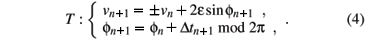
where Dt_n+1 = t_n+1 - t_n is given by the smallest positive solution of

The plus sign in equations above corresponds to case 1 and the minus sign to case 2. Note that Eq. (5) should be solved numerically.

The tangent map DT|_{(vn, fn)} = J_n (Jacobian matrix) is given by

where the right hand side was obtained from Eq. (4). Then, det J_n = ± .

The partial derivatives of v_n+1 and f_{n +1} with respect to f_n and v_n are determined from Eqs. (4) and (5).

We have then

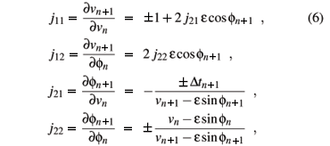
where the plus and minus signs refer to cases 1 and 2, respectively.

Thus the map has an invariant measure, namely (v - esinf) dv df. If e = 0 the measure is the usual canonical form dE dt.

B. The simplified model (SFUM)

Lieberman and Lichtenberg [2] introduced a simplified version of the Fermi accelerator. Now, we will suppose that the oscillating wall keeps a fixed position x_W = 1 but that, when the particle suffers a collision with it, the particle exchanges momentum and energy as if the wall were moving. This simplification carries the huge advantage of allowing us to speed up our numerical simulations very substantially as compared with those for the full model. It is valid when v_n >> e. Note that case 2 of the preceding subsection is impossible and the travel time between two impacts with the "oscillating wall" is simply given by 2/v_n, instead of Eq. (5).

Incorporating this simplification into the model, the map can be written as

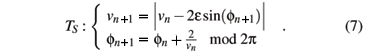
The modulus in the equation of the velocity was introduced artificially in order to prevent the particle leaving the region between the walls.

The coefficients of the Jacobian of the simplified map can be derived easily. Now, we have that det J = ±1 , implying that the SFUM is area preserving.

C. The phase space

It is well known that the energy in the FUM is bounded [4] because there are invariant spanning curves at sufficiently high energy (velocity). It is also known [2] that the map may have periodic orbits of low energy and thus KAM-like islands may be observed. Figs. 1 (a) and (b), show the typical phase space of the complete model, obtained by numerical iteration of Eq. (4).

The high energy region appears to be very well ordered and the low region seems to exhibit chaotic behavior. Note that there exists a first invariant spanning curve separating two regions that have different features: (a) the region above this curve is locally chaotic and structured by the existence of invariant spanning curves at high energy; and (b) below this curve the region (low energy) is globally chaotic, with KAM islands surrounded by an apparently ergodic sea.

The phase space of the SFUM, obtained by numerical iteration of Eq. (7), is shown in Fig. 1 (c) and (d). The structure of its phase space is essentially the same as that of the complete model.

III. SCALING ANALYSIS

A. Rescaling of the phase space

We consider first the SFUM. A naive estimation of the position of the lowest spanning curve may be obtained by transforming, locally, the simplified map into the Standard map by means of the coordinate change I_n = + 2, where v^* is a typical velocity characterizing the region of interest, followed by a linearization around this value. We obtain the Standard map equations

I_n+1 = I_n - K_eff sin f_n+1

f_n+1 = f_n + I_n

with an effective control parameter K_eff = . Note that the Standard map undergoes a transition between local and global chaos when K = K_c » 0.972. In Table I we list the values of K_eff related to the first (lowest) invariant spanning curve. For each e the lowest value of K_eff corresponds to the maximum value of the velocity on the spanning curve, and the highest corresponds to the minimum. Note also that K_eff has the same order of magnitude, independent of e. Moreover, both maximum and minimum values of K_eff seem to converge to K_c » 0.972 when e decreases.

The position of first invariant spanning curve of the FUM can be estimated as before. The values of K_eff for different values of e are also given in Table 1. Note that these values are basically the same as the ones obtained for each value of e of the simplified version.

It seems that the overall characteristics of the phase space are almost independent of e if the velocities are rescaled by 2, as can be seen in Fig. 1 for both models.

B. Lyapunov exponents of the chaotic sea

Let us now characterize the chaotic region below the first spanning curve, for both models. This region still contains islands with invariant curves surrounding stable periodic orbits but, outside these islands, we observe an apparently ergodic component. In our numerical simulations, the orbit of any initial condition outside the islands densely fills the same chaotic region. Moreover, as we will see, Lyapunov exponents for each of these initial conditions have the same value within the error bars. We will thus evaluate numerically the Lyapunov exponent l associated with this ergodic component. We choose an initial condition in the chaotic sea. Then, we use the exact form of the tangent map J ( Eq. (6) for the FUM ) and the triangularization algorithm as proposed in [28] to evaluate

Here, are the eigenvalues of DT^N = J_n, the product of the Jacobians of the map evaluated along the orbit.

We numerically estimate the positive Lyapunov exponent associated with the low energy region bellow the lowest spanning curve of the simplified model. For each value of e, we have chosen different initial conditions in the chaotic sea. A typical run is shown in Fig. 2 for e = 1 ×10^-4 and 10 different initial conditions. The positive Lyapunov exponent reaches a steady regime for each orbit and all runs seem converge to an average value.

Fig. 3 shows the average value of the positive Lyapunov exponent for different values of e. Note that the Lyapunov exponent barely seems to depend on e, since it changed only 17% in five decades of e.

The same procedure is applied to the FUM. The resulting positive exponents for different values of e have a similar behavior to the SFUM. Indeed, in four decades of e, the exponent changed also only by 17%. However, for the same value of e, the positive exponent of the complete model is roughly half the value of the exponent of the simplified model. This discrepancy could be related to more refined differences between the models.

The renormalization of the phase space, discussed in the previous subsection, is not only qualitative. The scaling factor is related to the existence of an effective parameter K_eff µ 4e/ v² . The high velocity regions correspond to small K_eff and thus are well organized and close to being integrable. Low energy regions are associated to large K_eff and thus associated with chaos. Well-organized and chaotic regions are present in each phase space, independently of e up to a size scaling factor. The transition occurs in the first invariant spanning curve when K_eff » K_c » 0.972. Moreover, even though we have studied a one parameter model which is completely integrable for e = 0, one cannot say that it becomes more chaotic by increasing e since the Lyapunov exponent is almost independent of e.

C. Scaling functions

The results of the previous section suggest that the chaotic sea can be described by rescaled variables. It means that scaling functions are an appropriate framework. Consider w(n,e,v₀) as a quantity, like velocity or energy, averaged over the initial phase f₀, and depending on the iteration number n, the amplitude e and the initial velocity v₀. The averaged quantity is a generalized homogeneous function [26], if for all values of the scaling factor l, the relation

is valid. Here, a, b and c are the scaling dimensions and lªn, l^be and l^c v₀ are the so called scaled variables.

First, let us consider v₀» 0, a simpler situation in which we have to deal with only two variables. In order to discuss the scaling behavior, we choose l = n^-1/a. Then, we have that w(n,e,0) = n^-1/aw(1,n^-b/ae,0) . The function w(1,n^-b/ae,0) can be written in terms of variable n as w(1,n^-b/ae,0) = g(n/n_x), where the characteristic iteration number n_x is given by

Note that there are two regimes: (a) small n (n << n_x) and (b) large n (n >> n_x).

In order to describe both regimes, we must know the behavior of g (or w(1,n^-b/ae,0)) for n << n_x and for n >> n_x. Consider first n << n_x. Usually we have that g » constant, implying that w µ n^-1/a. However the general behavior is g µ n^-by/ae^y, with the former case being obtained when y = 0. Therefore, we can write that

for n << n_x.

For large n we expect w to be idependent of n and to reach an asymptotic value. If the behavior of g in this regime is g µ n^-by'/ae^y', we must have that y' = -1/b, in order to reach such asymptotic value. For n >> n_x, we therefore have the following relationship

It is less straightforward to discuss the case v₀¹ 0. Again choosing l = n^-1/a, Eq. (8) can be written as

Note that we have now two characteristic iteration numbers. For very large n, we expect that w reaches an asymptotic value independently of the initial velocity, in such way that Eq. (11) remains valid. On the other hand, the behavior for small n can be very different of that described by Eq. (10).

We can relate the exponents c and b as follows. The initial velocity must be below the first spanning curve, implying that v_0,max ~ v^*. But K_eff = 4e/v^* is a quasi-invariant (K_eff » K_c » 0.972). We can thus rewrite the effective parameter in terms of scaled variables K_eff µ l^b-2c(e/v_0,max), and assume the invariability (b-2c = 0) to obtain that c = .

D. The average quantities

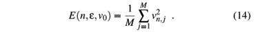
We will investigate the evolution of the velocity averaged in M initial phases, namely

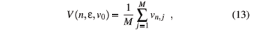
where j refers to a sample of the ensemble. In this ensemble we can also define the averaged dimensionless energy (E = 2 Energy/m

w²):

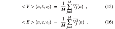
We are also interested in another kind of average. We first consider the average of velocity and the square velocity over the orbit generated from one initial phase f₀ namely (n) = v_i , and (n) = . Then we consider an ensemble of M different initial phases:

Finally, let us to introduce the roughness, namely

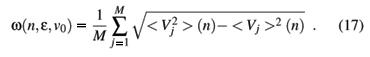
It is worth mentioning that the roughness is an extension of the formalism used to characterize rough surfaces[29].

E. Results for the simplified model

The behavior of the roughness is illustrated in Fig. 4(a) for two values of the parameter e, when the initial velocity is near zero. We can see that it grows for small iteration number n and then saturates at large n. The change between the two regimes is characterized by a crossover iteration number n_x. Note that different values of e generate different behaviors for short n. This indicates that the exponent y, defined in Eq. (10), is non-zero. In fact, the transformation w/e coalesces the two curves, as shown in Fig. 4(b). Therefore we have that y = 1.0(1). Moreover, for e = 1×10^-4 and n << n_x a best fit is shown in Fig. 4(a) and it furnishes that w(n,e,0) µ n^b e , with the growth exponent b = 0.5000(2). Other fits always furnish values for b around 0.5. After averaging over different values of the control parameter e in the range e Î [10^-4,10^-1], we then obtain b = 0.496(6). Then, we can conjecture that b = 1/2 and relate it to exponents a and b by Eq. (10). We obtain that - = 1/2.

From Fig. 4(a), we can also infer : (i) that for n >> n_x, the roughness reaches a saturation regime that is describable as w_sat(e) µ e ^a , where a is the so called roughening exponent [29]; and (ii) that the crossover iteration number n_x marking the approach to saturation is n_x(e,v₀) µ e ^z , where z is called the dynamical exponent.

The exponent a is obtained in the asymptotic limit of large iteration number, and it is independent of the initial velocity. Fig. 5(a) illustrates an attempt to characterize this exponent using the extrapolated saturation roughness. Extrapolation is required because, even after 10³n_x iterations, the roughness has still not quite reached saturation. From a power law fit, we obtain a = 0.512(3) » 1/2. Note that this is our worst average value because we have included data for large e. This best fit value approaches 1/2 as long we consider only small e. Using Eq. (11) we obtain -1/b = 1/2. Since - = 1/2, we have that 1/a = 1/2. Therefore we have determined all scaling dimensions, namely a = 2, b = -2 and c = b/2 = -1. From Eq. (9), we obtain the dynamical exponent z = a/b = -1. This exponent can also be found numerically. Fig. 5(b) shows the behavior of the crossover iteration number n_x as function of the control parameter e. The power law fit gives us that z = -1.01(2), in good accord with the previous scaling result. Since the fit is clearly worse for large values of the parameter e, we conclude that z = -1 for e small enough.

The scaling for v₀» 0 is demonstrated in Fig. 4, where two curves for the roughness in (a) are collapsed onto the universal curve seen in (c) when we normalize the quantities with the exponents a = 2 and b = -2. Note that we have two curves characterized by e₁ = 1×10^-4 and e₂ = 1 ×10^-3. Using Eq. (8), we obtain the scaling factor l = (e₂/e₁)^1/b and the appropiate renormalizations of the iteration number n₁ = l^-an₂ and roughness w₁ = lw₂.

Let us now discuss the scaling when v₀¹ 0. This case is better illustrated by the average velocity (see Fig. 6). Note that there are two characteristic iteration numbers, namely µ 1/e and µ /e². Since the maximum initial velocity inside the chaotic sea is v_0,max» 2e^1/2, the second scale has a maximum value of ( ~ 4). So two different kinds of behavior may occur, for < or ~ . When v₀ = 10^-6, we have » 0 and we can see in Fig. 6(a) that the curves for e = 10^-4 and e = 10^-3 show only two regimes: (i) a growth in power law for n << and (ii) the saturation regime for n >> . When v₀ = 10^-3 and e = 10^-4 we have that < and we can see for such curve in Fig. 6(a) three regimes: (i) for n << , the average velocity is basically constant; (ii) when < n < , the curve grows and begin to follow the curve of v₀ = 10^-6 and same e; (iii) for n >> we have the saturation regime. It is shown in Fig 6(b) that the collapse of the curves holds for v₀» 0 and v₀¹ 0, implying that the inferred scaling form V(n,e,v₀) with exponents a = 2, b = -2 and c = -1 is also correct.

We have also studied numerically the average energies E(n,e,v₀) and < E > (n,e,v₀). They have a similar scaling behavior. Since E ~ V², the exponents characterizing the energy a', b' and y' can be written in terms of those related to the average velocity and roughness as a' = 2a, b' = 2b and y' = 2y. Then, using Eqs. (10) and (11) it is easy to show that the scaling dimensions of average energies are a' = a/2 = 1, b' = b/2 = -1 and c' = c/2 = -1/2. These relationships were confirmed numerically.

F. Results for the complete model

The scaling dimensions of the complete model are the same as those obtained for the SFUM. To illustrate this fact, let us discuss the behavior of the energy < E > , first averaged over the orbit and then in the initial phase f₀.

Fig. 7(a) shows the behavior of < E > as a function of n for v₀ = 10^-6 and two values of the parameter e. A best fit for e = 1×10^-4 characterizes the initial growth with an exponent b' = 1.03(1). Since < E > µ e ², as shown in Fig. 7(b), we have that y' = 2.0. A plot of the saturation value of < E > as a function of e furnishes an exponent a' = 1.05(3). Therefore we can conjecture that a' = b' = 1 and y' = 2. Using Eqs. (10) and (11) we finally obtain that a' = 1, b' = -1 and c' = -1/2.

In Fig. 8(a) we have curves of < E > as functions of n for two values of e and different initial velocities. Using the exponents just discussed we obtain the collapse shown in Fig. 8(b). For v₀» 0 we can see that after an initial transient the scaling regime is established and the two curves collapse very well onto a universal one. When v₀¹ 0 we have also the scaling behavior. The other quantities (E, w and V) have similar scaling laws.

Finally, let us summarize our results for the Fermi-Ulam model. We characterized the chaotic region below the first invariant spanning curve (chaotic sea) in the transition from integrable (e = 0) to non-integrable (e ¹ 0). All results are valid for small oscillation amplitude e. The average quantities can be described by scaling functions with characteristic exponents. Since the positive Lyapunov exponent is almost independent of e, we cannot say that the system becomes more chaotic by increasing e.

J. K. L. da Silva, D. G. Ladeira, E. D. Leonel and S. O. Kamphorst thank to CNPq, CAPES and FAPEMIG, Brazilian agencies, for financial support.

[1] E. Fermi, Phys. Rev. 75 (6), 1169 (1949).

[2] A. J. Lichtenberg and M. A. Lieberman, Regular and Chaotic Dynamics, Appl. Math. Sci. 38, Springer-Verlag, New York (1992).

[3] M.A. Lieberman and A. J. Lichtenberg, Phys. Rev. A 5, 1852 (1971).

[4] R. Douady, Applications du théorème des tores invariants, Thèse de 3ème Cycle, Univ. Paris VII (1982).

[5] L. D. Pustil'nikov, Trudy Moskov. Mat. Obsc. 34 (2), 1 (1977); L. D. Pustil'nikov, Theor. Math. Phys. 57, 1035 (1983); L. D. Pustil'nikov, Sov. Math. Dokl. 35(1), 88 (1987); L. D. Pustil'nikov, Russ. Acad. Sci. Sb. Math. 82(1), 231 (1995).

[6] A. J. Lichtenberg, M.A. Lieberman and R. H. Cohen, Physica D 1, 291 (1980).

[7] E. D. Leonel and P. V. E. McClintock, J. Phys. A 38, 823 (2005).

[8] P. J. Holmes, J. Soun. Vib. 84, 173, (1982).

[9] R. M. Everson, Physica D 19, 355, (1986).

[10] E. D. Leonel and P. V. E. McClintock, J. Phys. A 38, L425 (2005).

[11] P. Seba, Phys. Rev. A 41, 2306 (1986).

[12] J. V. José and R. Cordery, Phys. Rev. Lett. 56, 290 (1986).

[13] S. T. Dembinski, A. J. Makowski and P. Peplowski, Phys. Rev. Lett. 70, 1093 (1993).

[14] S. R. Jain, Phys. Rev. Lett. 70, 3553 (1993).

[15] G. Karner, J. Stat. Phys. 77, 867 (1994).

[16] Z. J. Kowalik, M. Franaszek and P. Pieranski, Phys. Rev. A 37, 4016 (1988).

[17] S. Warr, W. Cooke, R. C. Ball and J. M. Huntley, Physica A 231, 551 (1996).

[18] E. Canale, R. Markarian, S. O. Kamphorst and S. P. de Carvalho, Physica D 115, 189 (1998).

[19] A. Loskutov and A. B. Ryabov, J. Stat. Phys. 108, 995 (2002).

[20] E. D. Leonel and P. V. E. McClintock, Chaos 15, 033701 (2005).

[21] J. L. Mateos, Phys. Lett. A 256, 113 (1999).

[22] G. A. Luna-Acosta, G. Orellana Rivadeneyra, A. Mendoza-Galván and C. Jung, Chaos, Solitons and Fractals 12, 349 (2001).

[23] E. D. Leonel and J. K. L. da Silva, Physica A 323, 181 (2003).

[24] E. D. Leonel and P. V. E. McClintock, Phys. Rev. E 70, 016214 (2004).

[25] E. D. Leonel, J. K. L. da Silva and S. O. Kamphorst, Physica A 331, 435 (2004).

[26] S. Ma, Modern Theory of Critical Phenomena, The Benjamin/Cummings Publishing Company, Massachusetts, (1976).

[27] E. D. Leonel, P. V. E. McClintock and J. K. L. da Silva, Phys. Rev. Lett. 93, 014101 (2004).

[28] J.-P. Eckmann and D. Ruelle, Rev. Mod. Phys. 57, 617 (1985).

[29] A. -L. Barabási, H. E. Stanley, Fractal Concepts in Surface Growth (Cambridge University Press, Cambridge, 1985).

Received on 25 October, 2005

Publication Dates

• Publication in this collection
  16 Oct 2006
• Date of issue
  Sept 2006

History

• Received
  25 Oct 2005