Experimentação e Simulação Tridimensional de Tubos AISI 304l Via Processo TIG em Operação em Regime Laminar Usando o Método dos Volumes Finitos

Experimental and 3D Numerical Simulation of In-Service AISI 304l Pipes by the Gtaw Process for Laminary Regime Using the Finite Volume Method

Resumos

Resumo

O objetivo deste trabalho é apresentar resultados experimentais e numéricos de soldagem de tubos AISI 304L em operação utilizando o processo TIG. Foi montada e construída uma bancada experimental para soldagem em operação que permite a montagem de um corpo de prova tubular de aço inoxidável AISI 304L e que utiliza água como como fluido de trabalho. Foram realizadas medições de temperatura na superfície interna do tubo, da vazão do fluido e da corrente e tensão de soldagem. Baseado nos dados experimentais obtidos da bancada experimental e, também, nas análises microscópicas, foi desenvolvido um modelo numérico utilizando o método de volumes finitos para prever o ciclo térmico de soldagem e as consequências deste aporte térmico sobre as transformações metalúrgicas. A fonte de energia (arco voltaico) foi modelada como uma superfície gaussiana móvel sobre uma elipsoide. Os resultados obtidos da simulação apresentaram uma boa concordância com os obtidos na bancada experimental, demonstrando que a simulação pode ser utilizada como uma ferramenta confiável para a previsão do processo de soldagem em operação.

Palavras-chave:
Processo TIG autógeno; Soldagem em operação; Tubos AISI 304; Volumes finitos

Abstract

The objective of this work is to present experimental and numerical results of the welding on in-service of AISI 304L pipes using the GTAW process. An experimental workbench was assembled and constructed with an AISI 304L stainless steel tube using water as a working fluid; temperature of the inner surface of the pipe, as well as the water flow rate, and the current and voltage of the welding process were acquired. Based on the information obtained with the experimental workbench and the microscopic analyses of the welding material, a numerical model was developed using the finite volume method to predict the thermal welding cycle and the heat-affected zone (HAZ). The welding energy was modeled as a movable Gaussian ellipsoid. The results obtained from the simulation were in good agreement with those obtained with the experimental workbench and therefore demonstrating that the proposed simulation can be used as a reliable tool for predicting the welding process on in-service stainless tubes.

Key-words:
Autogenous GTAW process; Welding process on in-service pipelines; AISI 304L tubes; Finite volume method

1. Introduction

In-service welding is considered the technique in which welding of equipment and pipelines are carried without the need for operational stops [¹]. In-service pipeline welding is a technique used in several areas of the industry. In this type of welding, operator safety and perforation of the wall of the tube, which can result in severe environmental and human damage, are the main concerns of this type of operation. The drilling of the tubing wall during the in-service welding process is mainly caused by the high density of locally deposited energy which can cause the melting of a large portion of the thickness, which combined with the internal pressure of the fluid can give rise to a perforation of the pipe in the welding region. Petrobras through the Technical Standard 2163 [¹] suggests that a numerical forecast of the maximum internal temperature of the wall must be performed and that this forecast value should not exceed 980°C (~1,253K). Another concern is the high cooling rate of welding material caused by forced convection of the fluid flow through the pipe. The high cooling rate in materials susceptible to martensite formation can promote the formation of martensite in the Heat-Affected Zone (HAZ) with high hardness, enhancing the formation of areas prone to crack formation [²]. Thus, an appropriate planning of heat intake during the welding process aiming to reduce the harmful effects of in-service welding becomes crucial.

Despite the complexity involved in the application of the boundary conditions, the large number of nonlinearities in the governing equations, and the change of material properties with temperature during the welding process, computational simulations are widely used and are effective for prediction of the welding processing [³]. Numerical simulations of the welding processes are also accurate and much cheaper than experimental procedures. Therefore, numerical methods are powerful tools for the evaluation of the phenomena involved and consequently avoid the formation of cracks in the HAZ or perforation of pipes on in-service welding.

Recent studies have shown some advances in research involving numerical simulations of in-service welding. Champagne and Pham [⁴] studied a three-dimensional heat transfer model using the element-free Galerkin (EFG) method, developed to predict the temperature field generated by a moving heat source. EFG methods are methods for solving partial differential equations with moving least square interpolators, which require only nodal data, without the need for element connectivity. The numerical results obtained by the EFG method were compared with those of the finite element method (FEM) and then validated with experimental results of arc welding. Good approximations were found between numerical and experimental results. Amori et al. [⁵] developed a numerical model using the three-dimensional finite element method to predict the temperature history along the thickness of the pipe wall using a computational code written in FORTRAN. They designed an experimental configuration to investigate the thermal history of an in-service welding process considering air as the working internal fluid in the pipe to be welded. Pipe drilling was investigated experimentally under the influence of gas flow rate, heat flow and defect depth presented in the pipe wall. The results showed good approximations between numerical predictions and experimental results. Dyck et al. [⁶] used the finite element method (FEM) to investigate the geometric effects of an in-service welding procedure of a connection, with the objective of evaluating the level of restrictions imposed by the thickness and diameter of both the connection and the main pipe. For this evaluation, a parameter was established, which was named the LoR (Level of Restrictions) parameter; the LoR parameter was quantified and compared by numerical simulation of multi-pass welding sequences for two configurations: a connection configuration in the multi-dimensional tube and a configuration using perpendicular plates as an alternative to the configuration in the tube. The results revealed a good approximation between numerical and experimental results and among the four variables investigated, the connection diameter is the most influential variable at the restriction level. As the connection diameter became smaller, the restriction level increased. Qian et al. [⁷] investigated the drilling mechanism during in-service welding through an exploratory study combining numerical experiments and simulations using the finite element method. The results showed that drilling was a type of fragile, intergranular rupture occurred in the cooling stage of in-service welding, starting in the partially melting zone and the cracks expanded along the weakened grain limits. When the cracks finally penetrated the inner wall, the rupture occurred.

Other studies were also important in the study of predictions of welding phenomena through numerical simulation. Armentani et al. [⁸] studied the two-dimensional temperature distribution in a welded joint using the finite element method. In this work, the influence of thermal and preheating properties on the residual stresses of welding material were investigated. Oddy and McDill [⁹] investigated the perforation in an in-service welding of a pressure vessel. They employed a thermomechanical three-dimensional and the equations were solved by the finite element method; the numerical results were compared with experimental data. They noted that drilling does not occur if the internal temperature does not exceed 980°C. Goldak et al. [¹⁰] used the finite element method to predict the three-dimensional temperature field in a pipe carrying natural gas. The results showed that the size and shape of the welding source has a significant impact on the calculation of penetration and temperature profile around the molten pool. Sabapathy et al. [³] performed a numerical investigation the drilling of gas pipelines in-service welding. A new mathematical description of the heat source for welding with manual coated electrode was introduced into his work, but limited data were provided for the temperature profiles. Xue et al. [¹¹] established a method to predict the rupture pressure and strain in operation under variable parameters using FEM. It has been shown that the rupture pressure of the project decreases when amount of heat input increases. Although limit the heat intake during in-service welding is an important issue to avoid drilling, the rapid cooling of welding can increase the crack susceptibility under certain specific conditions. Aissani et al. [²] investigated the determination of heat transfer characteristics for the GTAW welding process, combining an experimental approach and a three-dimensional simulation. The modeling of the heat source was performed by a moving Gaussian surface source exhibiting a bi-elliptical shape. This source was implemented in a three-dimensional model using the finite element method to calculate the heat flow and the temperature profiles. From the welding cycles and microstructural transformations, it was verified that the size of the melting zone is four times smaller than the size of the heat-affected zone. Anjos et al. [¹²] performed a numerical and experimental evaluation of an autogenous welding using a finite volume model to predict the temperature field in terms of welding cycles; the main objective was to predict the microstructures formed during the cooling process of welded parts. Therefore, CCT diagrams were compared with numerical and experimental temperature cycles. In that work, the 3D variation of the temperature field was considered, as well as the variation of thermal conductivity in relation to temperature.

The main focus of this work is to provide a numerical model using the finite volume method that can be used to predict the temperature field for both the welded material and the fluid flow considering laminar flow and therefore predict the thermal welding cycle, the welding zones, and the microstructure resulting from a tig autogenous welding of a 304L stainless steel tube. For the implementation of the model, data from an experimental in-service welding workbench were used to obtain volumetric flow rate, current, voltage, as well as the thermal cycle of an internal point of the welded region. The results of the workbench were also used to validate the numerical model. In addition, the microstructure was evaluated to compatibility with the thermal cycle obtained in numerical experiments and simulations.

2. Experimental Device

An experimental workbench was designed and assembled to perform autogenous GTAW automatic welding on the 304L austenitic stainless-steel tube, whose chemical composition and mechanical properties are presented respectively in Tables 1 and 2. The main characteristics of the workbench are shown in Figure 1. The following dimensions of the tube were used: length of 500 mm, external diameter equal to 48 mm, and thickness of 4 mm. Pure argon was used for welding with a flow rate of 12 l.min^-1 and the length of the weld bead was equal to 200mm.

Table 1
Standard composition Austenitic Stainless Steel 304L.

Composition (% of weight)
	C	Mn	P	S	Si	Cr	Ni
AISI 304L	0.03	2.0	0.045	0.03	1.0	18-20	8-12

Table 2
Minimum Values of Properties of Austenitic Stainless Steels 304L.

	Ultimate Strength (MPa)	Yield Strength Yield (MPa)	Elongation at break (%)	Reduction (%)
AISI 304L	480	170	40	50

Figure 1
Experimental workbench layout.

Welding was performed by adopting the following welding parameters (obtained from preliminary tests): current equal to 150A, voltage equal to 14 V, and welding velocity along the axial direction equal to 20 cm.min^-1 of welding speed. A tungsten electrode with 2% of thorium with a diameter of 2.4 mm was used. Automatic welding was performed in the flat position using a robotic arm integrated into an electronic source. The distance between the electrode tip and the welded surface was maintained between 2.5 to 3.0 mm.

Water was chosen as the internal working fluid because this fluid is widely used in industrial processes, its properties are well-known; in addition, it would be more suitable to preserve operator safety conditions. The water flow was kept continuous in the pipe using a submerged pump within a 1000 l water reservoir. A turbine-type flow sensor connected through cables to the data acquisition plate was used to acquire the flow rates. The flow control was performed with a valve at the entrance of the tube and the volumetric rate was maintained close to 70 l.h^-1.

The temperature measurement at the inlet and outlet of the tube and the wall of the tube close the welding bead was carried out using Type K thermocouples (Cromel/Alumel). All thermocouples were connected via cables to a data acquisition board, and the temperature was recorded automatically. The internal thermocouple was fixed with capacitive discharge welding equipment just below the welding in order to read the maximum internal temperature of the pipe. The pipe inlet and outlet thermocouples were fixed in connections to record the variation of the water temperature.

After welding, samples of the tube in the region of the weld, near the internal thermocouple, were prepared by cutting, sanding, polishing, and chemical attack with chromic acid (Composition: 10 grams of chromic acid + 90 milliliters of alcohol) to reveal the microstructure. With the samples prepared, the internal microstructure and welding zones were investigated using a light optical microscope (Model ZEISS Axio Observer) equipped with imaging analysis software and scanning electron microscopy (FEI Quanta 350 model).

3. Thermal Analysis

To obtain the temperature field for the fluid and for the welded region, it is necessary to solve the conservation equations of mass, momentum and energy; while the first aforementioned equations are solved only for the fluid domain, the energy equation need to be solved for the solid and fluid domains. Assuming axisymmetric, incompressible, and laminar flow with fluid properties independent of temperature, the equations of mass and momentum in the radial and axial directions of the pipe, written in the conservative form are given by:

$\frac{1}{r}\frac{\partial }{\partial r}\left(r{V}_r\right)+\frac{\partial }{\partial x}\left(V_x\right)=0$ (1)

$\frac{\partial }{\partial t}\left(\rho V_r\right)+\frac{1}{r}\frac{\partial }{\partial r}\left(r\rho V_r{V}_r\right)+\frac{1}{r}\frac{\partial }{\partial x}\left(r\rho V_x{V}_r\right)=-\frac{\partial p}{\partial r}+\frac{1}{r}\frac{\partial }{\partial r}\left[r\mu \left(\frac{\partial V_r}{\partial x}+\frac{\partial V_x}{\partial r}\right)\right]+\frac{1}{r}\frac{\partial }{\partial r}\left[2r\mu \frac{\partial V_r}{\partial r}\right]$ (2)

$\frac{\partial }{\partial t}\left(\rho V_x\right)+\frac{1}{r}\frac{\partial }{\partial r}\left(r\rho V_r{V}_x\right)+\frac{1}{r}\frac{\partial }{\partial x}\left(r\rho V_x{V}_x\right)=-\frac{\partial p}{\partial x}+\frac{1}{r}\frac{\partial }{\partial r}\left[r\mu \left(\frac{\partial V_r}{\partial x}+\frac{\partial V_x}{\partial r}\right)\right]+\frac{1}{r}\frac{\partial }{\partial x}\left[2r\mu \frac{\partial V_x}{\partial x}\right]$ (3)

In the above equations, r and x denote the radial and axial directions of the tube, V_x and V_r denote respectively, the axial (x) and radial (r) velocities, p is dynamic pressure, and μ is the dynamic viscosity of the fluid. The temperature field for the tube and fluid region can be represented by the following equation:

$\frac{\partial }{\partial t}\left(\rho T\right)+\frac{1}{r}\frac{\partial }{\partial r}\left(r\rho V_{r}T\right)+\frac{1}{r}\frac{\partial }{\partial x}\left(r\rho V_{x}T\right)=\frac{1}{r}\frac{\partial }{\partial r}\left[\frac{kr}{c_p}\frac{\partial T}{\partial r}\right]+\frac{1}{r^2}\frac{\partial }{\partial \theta }\left[\frac{kr}{c_p}\frac{\partial T}{\partial \theta }\right]+\frac{\partial }{\partial x}\left[\frac{k}{c_p}\frac{\partial T}{\partial x}\right]+S$ (4)

In the above equation, T denotes the temperature of the fluid or the region of the tube, k and cp denote respectively, the thermal conductivity and the specific heat of the fluid or tube, 𝜃 is the polar angle and S represents the welding energy per unit of volume and time. Note that while the velocity field is axisymmetric, the temperature field is 3D, that is, it varies with r, x, and 𝜃. It is also important to highlight that for the flow region S = 0 and that in the tube region the velocities are zero. The properties of the fluid were kept constant during the simulation, however the properties of the tube varied with the temperature. Further details will be provided in this section.

The welding energy is transmitted to the pipe through the electric arc and part of this energy is lost by convection and radiation to the environment and part by forced convection to the working fluid. The portion lost by forced convection for internal flow depends on the internal flow regime and is characterized by the Reynolds number. Considering that water in the experiments was at room temperature (300K), the volumetric flow rate of water equal to 70L.h^-1 (velocity equal to 0.015m.s^-1), the internal diameter of the pipe equal to 0.04m, the water density equal to 997kg.m^-3 and the water viscosity equal to 0,855x10^-3 Pa.s, the calculated Reynolds number is equal to 700 staying in the flow range of laminar regime, according to the objective of the analysis.

The velocity, temperature, and pressure of the internal fluid has a great effect on in-service welding. Much of the heat generated during the welding process and not delivered to the welded material will be transferred to the internal fluid flow. Thus, it is necessary to consider the influence of the characteristics of the internal flow on the safety of welding in operation. Xue et al. [¹¹] suggests that if the fluid has low viscosity and convection is forced, the number of Nusselt (Nu) can be calculated by Equation 5:

$Nu=0.023R{e}^{0.8}P{r}^{0.4}=\frac{hD}{k_f}$ (5)

in which Pr is the Prandtl number, h [W.m^-2. K^-1] is the coefficient of forced convection and k_f [W.m^-1.K^-1] is the thermal conductivity of the fluid. Considering the internal diameter of the pipe, the Pr equal to 5 (average between the constant heat condition and constant temperature) and k_f = 0.6128 W.m^-1.K^-1, the convection coefficient results in h = 126.62 W.m^-2K^-1.

The density, specific heat and thermal conductivity of the 304L stainless steel composition and temperature function were obtained from [¹³]. Therefore, it was assumed that the composition of 304L stainless steel as being 72%Fe, 19% Cr, and 9% Ni and that solid/liquid phase change temperature is 1700 K. The density and thermal conductivity of 304L steel for the solid and liquid phases are given by Equations 6 through 9:

$\rho =7.9841-2.650x{10}^{-4}-1.1580x{10}^{-7}{T}^2\left(solid\right)$ (6)

$\rho =7.5512-{\mathrm{1.1167.10}}^{-4}-1.5063x{10}^{-7}{T}^2\left(liquid\right)$ (7)

$k=8.116x{10}^{-2}+1.618x{10}^{-4}T\left(solid\right)$ (8)

$k=1.229x{10}^{-1}+3.248x{10}^{-5}T\left(liquid\right)$ (9)

Table 3 shows the specific heat (c_p) values used for 304L steel as a function of temperature [¹³].

Table 3
Specific heat values as a function of temperature.

Temperature [K]	Specific Heat Values [J.kg-1.K-1]
300	510.03
1700	698.73
1701	794.96
3000	794.96

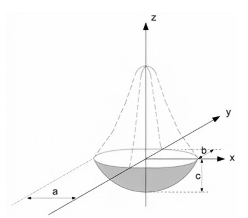
An important issue in the numerical simulation of welding processes is the choice of heat source geometry. In this work, welding was performed with the electric arc without material addition. The energy transferred from the arc to the tube was modeled as a 3D semi-ellipsoid gaussian with finite distribution with rays a, b, c as illustrated in Figure 2. This source presented in [¹⁴] is given by Equation 10:

Figure 2
Geometry of the Gaussian 3D volumetric source on an ellipsoid.

$q\left(x,y,z\right)=\frac{\eta VI}{abc\sqrt{\pi }}6\sqrt{3}exp\left(\frac{-3x^2}{a^2}\right)exp\left(\frac{-3y^2}{b^2}\right)exp\left(\frac{-3z^2}{c^2}\right)$ (10)

This source was selected due to its rapid implementation and it produce results as accurate as the other source formats [¹⁵]. The values of the geometric parameters of the ellipsoid rays (a, b, and c) were obtained by microscopic image measurements of the molten zone that resulted of the heat input of the welding arc. Welding efficiency was considered 65%, this value is based on an average of values used in the technical literature [¹⁶].

The boundary conditions were implemented according to the experimental conditions. On the outer surface of the tube the heat flow due to convection/radiation, q_n, is given by [¹⁷] as Equation 11:

$q_n=h_{\infty }\left(T-T_{\infty }\right)+\sigma ϵ\left(T^4-T_{\infty }^4\right)$ (11)

where h_∞ is the convective heat transfer coefficient [W.m^-2.K^-1], T_∞ is the ambient temperature, ε is the emissivity (0.82) [²] and σ is the Stephan-Boltzmann constant (σ = 5.67 x 10^-8 W.m^-2. K^-4). The simulation was divided into two phases: permanent regime for the fluid flow and transient for the heat transfer. The following boundary conditions were used for the fluid flow solution. At the entrance of the tube the axial velocity was kept constant and equal to 0.015 m.s^-1. This velocity was chosen based on the experiment carried out. At the tube outlet the dynamic pressure was maintained equal to atmospheric pressure.

For the transient heat transfer problem, the following boundary conditions were used: In the outer wall of the tube, the overall convection/radiation coefficient was fixed to 15 W.m^-2K^-1) as suggested in [²], [¹⁸]. The initial water temperature throughout the pipe was equal to 300K and the inlet value was 302 K, because the water reservoir was located externally and therefore exposed to the sun's heat which caused a small temperature rise. Also, we considered the material physical properties function of the temperature as given in Equations 4 through 7 and Table 3. Finally, it is important to stress that the heat source term as given by Equation 10 was inserted in the Fluent simulator using the Fluent interface named UDF (User defined function). For all the solutions obtained, residuals of the order of magnitude of (10^-8) were reached.

Figure 3 shows the geometry of the 304L stainless steel tube with the dimensions used in the experiment, the region where the welding was performed, and the position where thermocouple was fixed to acquire the temperature of the internal surface.

Figure 3
Geometry - dimensions and position of the internal thermocouple.

Equations 1 through 4 along with the initial and boundary conditions were solved by the finite volume method using the Ansys/Fluent commercial package. In the present work, solid and fluid domains were discretized with hexahedron elements [¹⁹]. A mesh refinement study was performed in order to assess that the results were independent of the mesh. The final mesh that provided independent welding cycles is shown in Figure 4. In order to adequately capture the temperature gradient at the interface of the internal wall and the fluid, a localized refinement of the mesh was performed, in this region.

Figure 4
Detail of the hexahedron mesh used in the simulation.

4. Results

4.1. Experimental procedure

Several GTAW autogenous welds were performed under the tube surface to obtain the thermal welding cycle values for the internal point of the pipe shown in Figure 3. The welding and water flow parameters are listed in Table 4. The measurements were continuously recorded in the welds performed, aiming to ensure the repeatability of the results.

Table 4
Welding parameters and water flow.

Parameter	Value
Current [A]	150
Voltage [V]	14
Welding velocity [cm.min-1]	20
Argon gas volumetric flow rate [L.min-1]	12
Water volumetric flow rate [L.H-1]	70

Figure 5 shows three welding cycles acquired in the thermocouple that was located in the inner wall, just below the welding zoned, please see Figure 3. It is observed that all the three cycles are very close to each other. In addition, it is noticed that the peak temperature of the three cycles was in the range 1036 - 1064 K, with a maximum difference of approximately 3%.

Figure 5
Thermal welding cycles.

Figure 6 shows the metallographic analysis performed in the 304L stainless steel. From Figure 6, it is possible to verify that the microstructure of the base metal of AISI 304L stainless steel consists mainly of austenite grains with the presence of a small amount of delta ferrite (elongated dark phase) [²⁰]. It is also possible to observe in the microstructure of 304L steel (as received) an austenite matrix with some dark particles which are reported as carbides [²¹].

Figure 6
AISI 304L stainless steel - base metal.

Figure 7 shows the lower interface of the fusion zone (FZ) and the heat-affected zone (HAZ). From this figure, it can be observed that the MZ is composed mainly of columnar dendrites close to the melting line, this is because of the high cooling rate that provides a rapid solidification [²²]. The region near the thermocouple has the same characteristics as the regions close to the ZF/ZAC interface. Through a CCT diagram of 304L steel, it is perceived that by the high cooling speed, mainly caused by the high rate of energy removed by the internal water flow that the microstructure corresponds to the thermal cycle agree with the ones shown in Figure 7. It is important to mention that the cooling time between the peak of temperature and the one close to room temperature was less than 1 minute.

Figure 7
FZ/HAZ interfaces.

Figure 8 shows a cut from the welding pool obtained through a SEM (Scanning Electron Microscope) that presents the measurements of the width and penetration of the weld. Table 4 shows the width and penetration for each weld performed, and the average of the former parameters. These values were important for the heat source parameters (Equation 10) used in the simulation.

Figure 8
Weld pool measurements - AISI 304L welding.

Table 5
Summary of macrography measurements.

	Width [mm]	Penetration [mm]
Welding 1	7.83	1.32
Welding 2	7.72	1.31
Welding 3	7.52	1.28
Average	7.69	1.30

4.2. Numerical simulations

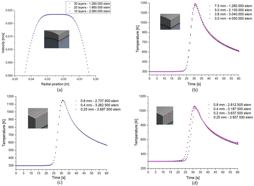
A mesh study refinement was conducted in order to ensure that the results were independent of the mesh. The meshes were refined in the region where the large temperature gradient are expected, region close to the welding and near the inner wall of the tube [²³].

Figure 9a shows the axial velocity in the region close to the welding bead. It is noticed that the axial velocity profile does not undergo major changes. Figure 9b, 9c, and 9d investigate the effect of the size of the element on the welding cycle at the location where the thermocouple was fixed. According to the previous tests the mesh used for numerical simulations has 3,187,500 elements.

Figure 9
Mesh refinement study. (a) Inner tube; (b) effect of the element width in the welding region; (c) effect of the element length in the welding region; and (d) effect of the element height in the welding region.

According to the melting pool measurements obtained by microscopy visualizations, the following parameters of the semi-ellipsoid gaussian with finite distribution were selected: width equal to 7.7 mm, penetration equal to 1.3 mm, and length equal 21 mm.

4.3. Results of simulations versus experimental data

Figure 10 shows the comparison of experimental and numerical thermal cycles in the position displayed in Figure 3. The maximum error between the experimental and numerical temperatures was around 10%, which from engineering point of view is an acceptable value. It is important to note that the peak temperature was in remarkably agreement to the experimental values as shown in Table 6. The largest difference between the experimental and the simulated results was verified for the heating phase, where we can clearly observe a delay in the numerical results. Such a difference can be caused by minor change in the thermocouple position. For the cooling phase, although minor difference in the experimental and numerical results were observed in the cooling phase, all curves presented the same trend. These results show the validity of the numerical model adopted. Finally, it is important to mention that the above results are consistent with the welding literature [²⁴], [²⁵].

Figure 10
Thermal Cycles - Experimental × Numeric - AISI 304L.

Table 6
Peak of temperature.

Step	Peak Temperature [K]
Welding 1	1036.776
Welding 2	1055.048
Welding 3	1064.031
Numerical Simulation	1039.509

Using the JMatPro software (license acquired by LPTS / UFC), a CCT chart was generated for AISI 304L stainless steel in order to assess whether the welding cooling curves, and the numerical simulation are consistent with the microstructure shown in the microscopy images. Figure 11 shows this assessment.

Figure 11
CCT chart AISI 304L (JMatPro).

Figure 12 presents a comparison of macrography region with the numerical temperature field. In order to performed such a comparison, the following temperatures were selected melting temperature = 1500K and important metallurgical changes = 1200K. It is noticed that the penetration has a very small difference, about 0.3 mm. This is an important result, because the criterion of safety evaluation, according to welding standards, are the maximum temperatures reached on the internal surface, which influence the penetration and possible weakening of the pipe wall. Regarding the width of the simulated melting zone a larger difference between experimental and numerical result was observed. However, this difference did not impact in the effect of the numerical approach in forecasting the possibly perforation of the tubing. Similar conclusions can be found in [²⁶].

Figure 12
Macrography × Temperature Profile - AISI 304L.

5. Conclusions

According to the results obtained from this paper, the following specific conclusions can be drawn:

• The finite volume method can be used for temperature forecasting of in-service welding, where there exist a strong coupling of energy delivered by the welding machine and the internal fluid flow that strongly impact the withdraw of energy from the workpiece by convection;

• Numerical simulation of GTAW welding in 304L stainless steel tubes shows that the semielliptical shape is a good approximation of the surface heat source. The associated dimensions of the elliptical shape are very important to obtain an accurate prediction of the temperature profile and as well as the peak of temperature reached. The best agreement of the numerical and experimental of thermal cycles was obtained with the following parameters and dimensions of the analytical heat source: a = 21.0 mm, b = 7.7 mm and c = 1.3 mm and efficiency of 65%;

• From the temperature field obtained, it was verified that the maximum internal temperature of the inner wall of the tube reached values up to 1039K. This predicted temperature is in a good agreement with the experimental value. The highest difference between the peak of temperature reached by the experimental and numerical welding cycles was about 2.3%, which is a very good forecast;

• The comparison between the observed and predicted dimensions of the welding pool, showed some minor difference in terms of the width and penetration. The main sources of the above differences are due, in part, to uncertainties regarding the external convection and convection in the melting pool. However, it is perceived that the numerical model predicted a penetration larger than the one observed in experimental procedure, which makes the simulation more conservative and therefore from the point of view of security is better;

• The microstructural analysis confirmed the observations of grain morphologies induced by heat at the analyzed microstructure and it is consistent with the results of the literature and CCT chart. Therefore, the modeling presented in this paper has the potential to be used in predicting microstructures resulting from in-service welding of the GTAW process.

Acknowledgements

Thanks to UFC, LPTS/UFC, Petrobras, FUNCAP, CAPES, CNPq for the financial support of this work.

References

• ¹
  Petrobras. Norma N-2163: revisão. Emissão e revisão de documentos de projeto. Rio de Janeiro; 2016 [access 4 nov. 2021]. Available from: http://www.petrobras.com.br/pt
  » http://www.petrobras.com.br/pt
• ²
  Aissani M, Guessasma S, Zitouni A, Hamzaoui R, Bassir D, Benkedda Y. Three-dimensional simulation of 304l steel GTAW welding process: contribution of the thermal flux. Applied Thermal Engineering. 2015;89:822-832. http://dx.doi.org/10.1016/j.applthermaleng.2015.06.035
  » http://dx.doi.org/10.1016/j.applthermaleng.2015.06.035
• ³
  Sabapathy P, Wahab MA, Painter M. Prediction of burn-through during in-service welding of gas pipelines. International Journal of Pressure Vessels and Piping. 2000;77(11):669-677. http://dx.doi.org/10.1016/S0308-0161(00)00056-9
  » http://dx.doi.org/10.1016/S0308-0161(00)00056-9
• ⁴
  Champagne O, Pham XT. Numerical simulation of moving heat source in arc welding using the element-free galerkin method with experimental validation and numerical study. International Journal of Heat and Mass Transfer. 2020;154:119633. http://dx.doi.org/10.1016/j.ijheatmasstransfer.2020.119633
  » http://dx.doi.org/10.1016/j.ijheatmasstransfer.2020.119633
• ⁵
  Amori DKE, Hussain MN, Hilal HB. Thermal analysis of in-service welding process for pipeline. Journal of Petroleum Research and Studies. 2019;9(1):1-120. http://dx.doi.org/10.52716/jprs.v9i1.270
  » http://dx.doi.org/10.52716/jprs.v9i1.270
• ⁶
  Dyck J, Guest S, Kohandehghan A, Lepine S. Simulating in-service welding of hot-tap branches to quantify the effect of geometry on level of restraint. In: Proceedings of the 2018 12th International Pipeline Conference; 2018 September 24-28; Calgary, Alberta. New York: ASME; 2018. (Vol. 3: Operations, Monitoring, and Maintenance; Materials and Joining). http://dx.doi.org/10.1115/IPC2018-78600
  » http://dx.doi.org/10.1115/IPC2018-78600
• ⁷
  Qian W, Yong W, Tao H, Hongtao W, Shiwei G, Laihui H. Study on the failure mechanism of burn-through during in-service welding on gas pipelines. Journal of Pressure Vessel Technology. 2019;141(2):024501. http://dx.doi.org/10.1115/1.4042461
  » http://dx.doi.org/10.1115/1.4042461
• ⁸
  Armentani E, Esposito R, Sepe R. The influence of thermal properties and preheating on residual stresses in welding. International Journal of Computational Materials Science and Surface Engineering. 2007;1(2):146-162. http://dx.doi.org/10.1504/IJCMSSE.2007.014870
  » http://dx.doi.org/10.1504/IJCMSSE.2007.014870
• ⁹
  Oddy A, McDill J. Burn through prediction in pipeline welding. International Journal of Fracture. 1999;97(1-4):249-261. http://dx.doi.org/10.1023/A:1018369304971
  » http://dx.doi.org/10.1023/A:1018369304971
• ¹⁰
  Goldak J, Mocanita M, Aldea V, Zhou J, Downey D, Dorling D. Predicting burn-through when welding on pressurized natural gas pipelines. Pressure Vessels and Piping Division. 2000;410:21-28.
• ¹¹
  Xue X, Zhu J, Sang Z. Study on design pressure of in-service welding pipes. Science in China Series E: Technological Sciences. 2006;49(4):434-444. http://dx.doi.org/10.1007/s11431-006-2005-2
  » http://dx.doi.org/10.1007/s11431-006-2005-2
• ¹²
  Anjos F, Fernandes BRB, Araújo ALS, Miranda HC, Marcondes F. Numerical investigation of transient temperature distribution in arc welding process. In: Proceedings of the 13th Brazilian Congress of Thermal Sciences and Engineering (ENCIT2010); 2010; Uberlândia. Rio de Janeiro: ABCM; 2010. p. 9.
• ¹³
  Kim CS. Thermophysical properties of stainless steels. 1st ed. Virginia: National Technical Information Service; 1975. http://dx.doi.org/10.2172/4152287
  » http://dx.doi.org/10.2172/4152287
• ¹⁴
  Guimarães PB. Estudo do campo de temperatura obtido numericamente para posterior determinação das tensões residuais numa junta soldada de aço ASTM AH36 [tese de doutorado]. Recife: Universidade Federal de Pernambuco; 2010.
• ¹⁵
  Hashemzadeh M, Chen B-Q, Soares CG. Comparison between different heat sources types in thin-plate welding simulation. In: Soares CG, Pena FL, editors. Developments in maritime transportation and exploitation of sea resources. 1st ed. New York: CRC Press; 2014. p. 329-335.
• ¹⁶
  Kou S. Welding metallurgy. 2nd ed. Hoboken: John Wiley & Sons; 2003. 466 p.
• ¹⁷
  Masumi VA, Ali V. Numerical analysis of the burn-through at in-service welding of 316 stainless steel pipeline. International Journal of Pressure Vessels and Piping. 2013;105:49-59.
• ¹⁸
  Goldak J, Akhlaghi M. Computational welding mechanics. Boston: Springer; 2005.
• ¹⁹
  Biswas R, Strawn RC. Tetrahedral and hexahedral mesh adaptation for cfd problems. Applied Numerical Mathematics. 1998;26(1-2):135-151. http://dx.doi.org/10.1016/S0168-9274(97)00092-5
  » http://dx.doi.org/10.1016/S0168-9274(97)00092-5
• ²⁰
  Lima IL, Silva GM, Chilque ARA, Schvartzman MMAM, Bracarense AQ, Quinan MAD. Caracterização microestrutural de soldas dissimilares dos aços ASTM A-508 e AISI 316L. Soldagem e Inspeção. 2010;15(2):112-120. http://dx.doi.org/10.1590/S0104-92242010000200005
  » http://dx.doi.org/10.1590/S0104-92242010000200005
• ²¹
  Osoba L, Ekpe I, Elemuren R. Analysis of dissimilar welding of austenitic stainless steel to low carbon steel by GTAW welding process. International Journal of Metallurgical and Materials Science and Engineering. 2015;16.
• ²²
  Queiroz A, Fernandes M, Silva LM, Demarque R, Oliveira EM, Ellem PS, et al. Study of the microstructure of aisi steel 304l in WZ, HAZ and BM after welding in the gmaw process. American Journal of Engineering Research. 2017;6:433-438.
• ²³
  Maliska CR. Transferência de calor e mecânica dos fluidos computacional. 2nd ed. Rio de Janeiro: LTC; 2017. 440 p.
• ²⁴
  Li C, Wang Y. Three-dimensional finite element analysis of temperature and stress distributions for in-service welding process. Materials & Design. 2013;52:1052-1057. http://dx.doi.org/10.1016/j.matdes.2013.06.042
  » http://dx.doi.org/10.1016/j.matdes.2013.06.042
• ²⁵
  Huang Z, Tang H, Ding Y, Wei Q, Xia G. Numerical simulations of temperature for the in-service welding of gas pipeline. Journal of Materials Processing Technology. 2017;248:72-78. http://dx.doi.org/10.1016/j.jmatprotec.2017.05.008
  » http://dx.doi.org/10.1016/j.jmatprotec.2017.05.008
• ²⁶
  Liu W, Ma J, Kong F, Liu S, Kovacevic R. Numerical modeling and experimental verification of residual stress in autogenous laser welding of high-strength steel. Lasers in Manufacturing and Materials Processing. 2015;2(1):24-42. http://dx.doi.org/10.1007/s40516-015-0005-4
  » http://dx.doi.org/10.1007/s40516-015-0005-4

Datas de Publicação

• Publicação nesta coleção
  17 Dez 2021
• Data do Fascículo
  2021

Histórico

• Recebido
  09 Dez 2020
• Aceito
  02 Ago 2021