Hybrid kriging methods for interpolating sparse river bathymetry point data

Métodos híbridos de krigagem para interpolação de levantamentos batimétricos fluviais

ABSTRACT

Terrain models that represent riverbed topography are used for analyzing geomorphologic changes, calculating water storage capacity, and making hydrologic simulations. These models are generated by interpolating bathymetry points. River bathymetry is usually surveyed through cross-sections, which may lead to a sparse sampling pattern. Hybrid kriging methods, such as regression kriging (RK) and co-kriging (CK) employ the correlation with auxiliary predictors, as well as inter-variable correlation, to improve the predictions of the target variable. In this study, we use the orthogonal distance of a (x, y) point to the river centerline as a covariate for RK and CK. Given that riverbed elevation variability is abrupt transversely to the flow direction, it is expected that the greater the Euclidean distance of a point to the thalweg, the greater the bed elevation will be. The aim of this study was to evaluate if the use of the proposed covariate improves the spatial prediction of riverbed topography. In order to asses such premise, we perform an external validation. Transversal cross-sections are used to make the spatial predictions, and the point data surveyed between sections are used for testing. We compare the results from CK and RK to the ones obtained from ordinary kriging (OK). The validation indicates that RK yields the lowest RMSE among the interpolators. RK predictions represent the thalweg between cross-sections, whereas the other methods under-predict the river thalweg depth. Therefore, we conclude that RK provides a simple approach for enhancing the quality of the spatial prediction from sparse bathymetry data.

Index terms:
Geostatistics; spatial prediction; regression kriging; riverbed morphology

RESUMO

Modelos de terreno de rios são usados para análise de mudanças geomorfológicas e para simulações hidrológicas. Estes modelos são interpolados a partir de pontos batimétricos. A batimetria fluvial é geralmente conduzida através de seções transversais, o que pode acarretar em uma malha amostral esparsa. Métodos híbridos de krigagem, como krigagem por regressão (KR) e co-krigagem (CK), empregam a correlação com preditores auxiliares, além da auto-correlação entre variáveis, na predição da variável resposta. Neste estudo, sugere-se que a distância ortogonal de um ponto até a linha de centro do talvegue de um rio pode ser usada como covariável para KR e CK. Considerando-se que a variabilidade da cota do leito do rio é abrupta transversalmente a direção do fluxo, espera-se que quanto maior a distância euclidiana de um ponto até o talvegue, maior será sua elevação. O objetivo deste estudo foi avaliar o uso da covariável proposta em métodos híbridos de krigagem para a predição espacial da topografia do leito de rios. Para tanto, foi realizada uma validação externa, em que seções transversais foram usadas para interpolação e dados levantados entre as seções consistiram na amostra de teste. Os resultados da KR e CK foram comparados aos da krigagem ordinária. A KR apresentou a menor REQM. No mapa resultante da KR, o talvegue foi preservado nas lacunas não amostradas entre as seções, enquanto os demais métodos subestimaram a profundidade do talvegue nestes espaços. Assim, conclui-se que a KR pode melhorar a predição espacial de dados batimétricos fluviais.

Termos para indexação:
Geoestatística; predição espacial; krigagem por regressão; morfologia fluvial.

INTRODUCTION

River terrain models, which represent the submerse fluvial topography in a continuous manner, are useful for hydrologic simulations, as well as for the assessment of sediment transport and geomorphologic changes (Merwade, 2009; Glenn et al., 2016). Such models are usually generated by interpolating discrete point data, obtained from bathymetric or topographic surveys (Legleiter; Kyriakidis, 2008). Although LiDAR technology and multi-beam-echo-sounder sonar systems can provide high-resolution bathymetry data, single-beam-echo-sounders (SBES) offer a cost effective alternative for water depth measurements (Jha; Mariethoz; Kelly, 2013). Nevertheless, extensive sampling is still costly and time consuming. Therefore, river bathymetry is traditionally surveyed through cross-sections, which can be quickly recorded, using SBES sonar systems (Schäppi et al., 2010; Glenn et al., 2016).

However, cross-sectional sampling patterns may not lead to precise river terrain models. One of the difficulties is that cross-sections can be isolated and widely spaced, which increases the gaps of unsampled areas, and reduces the quality of the spatial prediction. River morphology is another complicator regarding the interpolation of bathymetry data. According to Merwade, Maidment and Goff (2006), river bed topography is anisotropic: the channel elevation variability is greater transversely to the flow direction than it is along the flow direction; also, such anisotropy is not spatially consistent, given the river sinuosity.

In order to overcome these issues, some researchers have suggested that the spatial trend in river channels could be modeled by converting the Cartesian (x,y) coordinate system into a channel-centered (s, n) spatial referenced system, where the s-axis is oriented along the flow direction and the n-axis is perpendicular to the flow (Goff; Nordfjord, 2004; Merwade; Maidment; Hodges, 2005; Legleiter; Kyriakidis, 2008). Once this transformation is done, several functions, such as polynomial regression, splines and probability density function, can be used to remove the data spatial trend (Merwade, 2009).

Nevertheless, coordinate transformation is not a common automatic feature for Geographic Information Systems (GIS), requiring some programming efforts that may not always be feasible. Hence, although sophisticated geostatisical techniques have been developed for interpolating bathymetric data (Legleiter; Kyriakidis, 2008; Merwade; Cook; Coonrod, 2008; Merwade, 2009), such techniques require a high level of user experience, and some users still rely on mechanical spatial prediction methods (Albertin et al., 2010; Miranda; Scarpinela; Mauad, 2013). Such methods, although simple and flexible, can be considered subjective and empirical, and provide no intrinsic estimation of the model error (Hengl, 2009).

In geostatistics, kriging techniques are considered to offer the best unbiased linear predictions (BLUP). That is, the linear equations from the kriging system provide estimations with a mean residual error equal to 0 and with minimum variance (Isaaks; Srivastava, 1989; Oliver; Webster, 2014). Hybrid kriging methods, such as co-kriging (CK) and regression kriging (RK), employ not only the spatial auto-correlation of the target variable, but also the inter-variable correlation, and the correlation with auxiliary predictors (Odeh; McBratney; Chittleborough, 2006; Hengl, 2009). Therefore, auxiliary maps with spatially exhaustive information are used to improve the predictions based on point observations of the target variable (Hengl; Heuvelink; Rossiter, 2007). Hybrid kriging methods have been widely used in several environmental sciences, such as topographic modeling (Hengl et al., 2008), soil science (Odeh; McBratney; Chittleborough, 2006; Zhu; Lin; 2010; Watt; Palmer, 2012; Qi-Yong et al., 2014), meteorology (Joyner et al., 2015) and marine sedimentology (Jerosch, 2013).

However, an important difference between RK and CK regards the assumption of stationarity of modeled field. In CK, as in the case of ordinary kriging (OK), the target variable is treated as a realization of a stationary random process, which varies in the same degree over a region of interest (Oliver; Webster, 2015). Therefore, in such methods, the mean response of the process is considered to be constant within the study area. On the other hand, the basic principle of RK is that the deterministic trend component of the spatial variability of the target variable can be modeled by a regression from spatially referenced covariates (Diggle; Ribeiro Jr., 2007). Hence, in RK, the target variable data is treated as non-stationary in the mean, and only the residuals from the modeled trend are consireded to be starionary (Webster; Oliver, 2007).

In this study, we hypothesize that, when dealing with sparse cross-sectional river bathymetry data, the orthogonal distance to the river centerline can be used as a covariate - or auxiliary variable, for hybrid kriging methods. Instead of converting the Cartesian coordinate system into a channel oriented system, we use the proposed auxiliary variable as a proxy for modeling the spatial trend of river bed topography. The covariate is employed for RK and CK. We compared the performance of these techniques with the results from OK, using datasets from three river reaches at the state of Minas Gerais, Brazil.

MATERIAL AND METHODS

Study area and bathymetric survey

This study is based on a bathymetric survey of the Funil hydroelectric power plant reservoir, located between the municipalities of Lavras and Perdões, in the southern region of the state of Minas Gerais, Brazil (Figure 1). The power plant started operating in 2003 and has been submitted to unexpectedly high sedimentation rates, especially due to sediments transported by the Mortes River (Figure 1).

Figure 1:
Study area: a) Grande River reach; b) Capivari River reach; c) Mortes River reach. Arrows indicate river flow direction. Transversal cross-sections are used for spatial prediction and longitudinal cross-sections are used for testing.

The survey was conducted in January 2015 as part of a reevaluation study of the water storage capacity of the Funil reservoir. A SBES attached to a motorized boat was used to measure water depth at (x,y) point locations. The survey was executed through cross-sections, transversely and longitudinally to the river flow direction (Figure 1). For each cross-section, water level was measured using Real Time Kinetics Global Positional System (RTK GPS) technology. The base of the device was fixated on a georeferenced mark, and the rover connected to the boat. The river bed elevation values (z) for each (x,y) point were calculated by subtracting water level from water depth.

Three river reaches were selected for this study according to the availability of validation data, i.e. the longitudinal sections which were surveyed between the transversal cross-sections (Figure 1). The Mortes and Capivari Rivers are tributaries to the Grande River, where the Funil dam is located. All reaches present a sparse and irregular cross-sectional sampling pattern (Table 1).

Table 1:
Data summary of the bathymetric survey on Capivari, Grande and Mortes River reaches. Mean and standard deviation refer to measured riverbed elevation (m).

River name	Reach lenght (km)	Mean width (m)	Mean cross-section spacing (m)	Points (total)	Mean (m)	Std. Dev. (m)	Min .	Max.
Capivari	1.49	40	71	634	803.72	1.32	799.53	807.43
Grande	1.97	288	152	2018	795.31	4.95	779.53	807.23
Mortes	1.22	144	122	918	805.24	1.39	799.23	807.53

Although the study area is located in a reservoir, the reaches still preserve river morphology. The motivation for this study came precisely from the fact that, when interpolating the Funil reservoir bathymetry data, we came to notice that most of the flooded area still maintains river morphology, which brings us back to all the obstacles previously discussed, regarding river bed spatial modeling.

Orthogonal distance to centerline

The spatial variability of river bed topography is abrupt transversally to the water flow direction (Figure 2). Due to such morphologic characteristic, it is expected that the greater the orthogonal distance of a (x,y) point to the river thalweg centerline, the greater the river bed elevation (z) will be.

Figure 2:
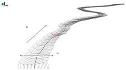
3D mesh of a river channel: bed elevation variability is smoother along flow direction (a), than across flow direction (b).

The river thalweg, i.e. a centerline along the lowest elevations of the water flow direction, is identified using a simplified adaptation of the methodology suggested by Merwade, Maidment and Hodges (2005). Firstly, a mechanical method with low computational demand is used to interpolate the observed point data. Secondly, the symbology of the points is altered according to the elevation values (z), which allows the visual identification of the thalweg within the cross-sections. Finally, the centerline is manually drawn, using editing tools, following the lowest values from the interpolated surface and the point symbology.

The orthogonal distance to the centerline is obtained through the Euclidean Distance tool, from ArcMap 10.1 (ESRI, 2011), which generates a grid raster where the cell values represent the minimum distance of a given location to a given vector (in this case, the centerline). Since the grid cell resolution of such raster is arbitrary, we evaluate the results from 1, 3, 5, and 10 m. Coarser resolutions are computationally less demanding, but can lead to generalizations which may hamper a precise estimation of the distance to centerline at the surveyed point observations.

The grid cell values generated by the Euclidean Distance tool are extracted at the sampled locations of the target variable. A regression model is then adjusted for bed elevation (Y) in function of the orthogonal distance to the centerline (X) for each river reach.

Data analysis

We evaluate the spatial trend of the datasets using the geostatistical analyst toolset of ArcGIS 10.1 (ESRI, 2011). A polynomial regression on coordinates is performed in order to model the data trend for the OK and CK methods.

For the kriging methods, the semivariograms are modeled after plotting the semivariances (γ) between the sampled values of the target variable (Hengl, 2009) (Equation 1):

$\gamma \left(h\right)=\frac{1}{2}E\left[{\left(z\left(s_i\right)-z\left(s_i+h\right)\right)}^2\right]$ (1)

where: z(s _i ) is the value of the target variable at a given location and z(s _i + h) is the value of the variable at a distance h.

For CK, the cross-covariogram is plotted according to Equation 2 (Webster; Oliver, 2007):

$C\left(h\right)=E\left[\left(z\left(s_i\right)-{\mu }_z\right)*\left(y\left(s_i+h\right)-{\mu }_y\right)\right]$ (2)

where: z(s _i ) is the value of the target variable at a s _i location; y(s _i + h) is the value of the co-variable y at a distance h; μ_z is the mean response of the target variable z and μ_y is the mean response of the co-variable y.

Kriging methods

All of the described kriging methods in this study are performed using the geostatistical analyst of ArcGIS 10.1 (ESRI, 2011).

In OK, the spatial prediction of a target variable (z) at an unsampled location (s ₀ ) is calculated as Equation 3:

$z^{*}\left(s_o\right)={\displaystyle \sum }_{i=1}^n{\lambda }_{i}z\left(s_i\right)$ (3)

where: n is the number of s _i observations of the target variable, and λ_i are the kriging weights chosen to minimize error variance (σ² ) (Equations 4 and 5) between sampled (s _i ) and estimated values (s ₀ ) (Oliver; Webster, 2014):

where: φ is the Lagrange multiplier, which optimizes kriging variance (Odeh; Mcbratney; Chittleborough, 2006).

$z^{*}\left(s_o\right)={\displaystyle \sum }_{i=1}^n{\lambda }_{i}z\left(s_i\right)$ (4)

${\displaystyle \sum }_{i=1}^n{\lambda }_i=1$ (5)

CK estimations are based the spatial auto-correlation of the target variable and the auxiliary variables (Isaaks; Srivastava, 1989) (Equation 6):

$z^{*}\left(s_o\right)={\displaystyle \sum }_{i=1}^n{a}_{i}z\left(s_i\right)+{\displaystyle \sum }_{j=1}^m{b}_{j}w\left(s_j\right)$ (6)

where: n is the number of s _i observations of the target variable z; m is the number of s _j observations of the auxiliary variable w, and a _i and b _j are the co-kriging weights.

RK predicts the values of a target variable z at an unsampled location s ₀ as the sum of the deterministic component of the signal process estimated by a fitted model plus the residual of such model (Equation 7), which is interpolated using ordinary kriging or simple kriging (Hengl; Heuvelink; Rossiter, 2007; Hengl; Heuvelink; Stein, 2004):

$\widehat{z}\left(s_o\right)=\widehat{\beta }\left(s_o\right)*q\left(s_0\right)+{\displaystyle \sum }_{i=1}^n{\lambda }_i\left(s_0\right)*e\left(s_i\right)$ (7)

where:

$\widehat{\beta }\left(s_o\right)$

are the regression coefficients from the deterministic component; q(s _o ) is the auxiliary variable at s _o ; w _i (s _o ) are the kriging weights, and e(s _i ) are the regression residuals.

In this study, the computational steps for the RK method can be summarized as:

1. Once a regression model of the target variable (channel elevation) in function of the covariate (distance to centerline) is fitted, the adjusted equation is applied to the auxiliary grid raster, using map algebra tools;

2. The regression residuals are calculated by subtracting the observed values of the target variable from the ones estimated by the model;

3. The residuals from the model are interpolated by OK;

4. The regression model grid raster is added to the interpolated residual surface using map algebra tools.

For all kriging methods a search neighborhood is standardized by setting a unique maximum number of 50 neighbors for interpolation (maximum value accepted by the software). According to Merwade, Maidment and Goff (2006), the accuracy of OK predictions for river bathymetry increases with the number of kriging neighboors.

Validation

The spatial prediction techniques are evaluated based on an external validation. The training dataset is the cross-section point data, whereas the testing dataset is surveyed along flow direction, between the transversal cross-sections. Such form of validation is performed in order to mimic a traditional cross-sectional survey, as suggested by Merwade, Maidment and Goff (2006).

Model performance was evaluated according to the residual Mean Error (ME), Root Mean Squared Error (RMSE), and Relative Absolute Error (RAE) (Bennet et al., 2013).

RESULTS AND DISCUSSION

The orthogonal distance to river centerline presents a significant positive correlation with river bed elevation on all the evaluated grid cell resolutions, at all river reaches (p < 0.05). We use the 1 m resolution raster as the auxiliary map for the RK method, in order to preserve the most accurate estimations of the distance to centerline. However, the results indicate that coarser resolutions might also be used.

Due to the correlation between the orthogonal distance to centerline and channel elevation, part of the spatial variability of river bed topography can be deterministically modeled. At the Mortes River reach, 63% of the spatial prediction is modeled according to a second-degree polynomial regression of elevation as a function of the orthogonal distance to river centerline. For the Grande River dataset, the linear regression from the auxiliary variable accounts for 53% of the river bed spatial variability. The Capivari River reach displays the lowest correlation between auxiliary and target variable, with a coefficient of determination of 40%, based on a second-degree polynomial model. Such behavior is most likely related to the sinuosity of this reach: the thalweg shifts from the outside of the meanders to the center of the channel, which leads to heterogeneous relation patterns between elevation and distance to centerline (Figure 3).

Figure 3:
Riverbed elevation models of the Capivari reach. OK: ordinary kriging; CK: co-kriging; RK: regression kriging.

The trend analysis of the Grande River reach demonstrates the effects of the thalweg and bed slope on the river spatial trend. Given that flow direction is roughly oriented from South to North, trend analysis showed a decrease in channel elevation with the increase of the Y coordinate, due to river bed slope (Figure 4). Such trend had an overall smooth behavior, except in the northern portion of the segment, where elevation decreases more abruptly. The trend in the direction of the X coordinate is much more evident. Figure 4 demonstrates how river bed elevation, clearly influenced by the river thalweg, is lower in the central region of the scatter plot.

Figure 4:
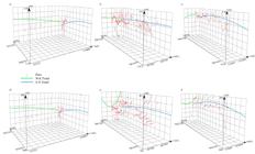
Spatial trend of riverbed elevation (d, e, f) and of the residuals from the regression of elevation in function of distance to centerline (a, b, c). Capivari reach (a, d); Grande reach (b, e); and Mortes reach (c, f). The vertical axis represents the value of the variable. Data points are projected on an east-west and north-south plane. Trend lines are best fitted polynomials that represent the spatial trend in each direction.

The regression from the auxiliary variable is able to model the river bed spatial trend adequately at the Grande and Mortes reaches. The residuals from the regression models display much smoother trend lines than the target variable, which is specifically evident in the case of Grande River reach (Figure 4). Such behavior is not so clear in the Capivari reach, which can be explained by the lowest correlation between orthogonal distance to centerline and channel elevation at the river segment (Figure 4).

The semivariograms for all the reaches and kriging techniques are fitted into a stable model (Figure 5). The sill values of the residual semivariograms are, on average, 25% lower than the ones from the target variable semivariograms, which indicates that the feature-space structure has decreased due to the effective removal of the external drift (Hengl; Heuvelink; Stein, 2004; Hengl; Heuvelink; Rossiter, 2007). The cross-variances are overall positive, given that the orthogonal distance to centerline presented a positive correlation with riverbed elevation. However, some negative values are displayed in the experimental cross-variograms as the lag distance increases, in both the Capivari and Mortes reaches, probably as a result of the thalweg shift along the flow direction.

Figure 5:
Semivariograms (a, b, c) and crossed-covariograms (d, e, f). Capivari reach (a, d); Grande reach (b, e); and Mortes reach (c, f).

The results from the external validation show that the spatial prediction methods yielded negative ME values at all analyzed reaches (Table 2). That is, the observed values from the testing datasets are higher than the ones predicted. Such results indicate a slight bias in the predictions, caused by an underestimation of the river thalweg depth between the cross-sections. At the Grande Rive reach, where cross-sections are more widely spaced, the ME departs farther from zero. RK exhibits ME values which are closer to zero, indicating a better representation of the channel at the unsampled intervals.

Table 2:
Validation statistics of the different methods and reaches.

River name	OK			CK			RK
	ME	RMSE	RAE	ME	RMSE	RAE	ME	RMSE	RAE
	---------m--------			---------m--------			---------m--------
Capivari	-0.23	0.75	0.52	-0.25	0.72	0.52	-0.11	0.64	0.42
Grande	-0.34	3.18	0.65	-0.43	2.94	0.62	-0.26	2.74	0.53
Mortes	-0.12	0.77	0.60	-0.10	0.78	0.79	-0.09	0.63	0.58

• Legend: OK: ordinary kriging; CK: co-kriging; RK: regression kriging; ME: Mean Error; RMSE: Root Mean Squared Error; RAE: Relative Absolute Error.

The external validation displays a consistent behavior of the spatial prediction methods regarding the RMSE (Table 2). At the Grande and Capivari reaches the highest RMSE values are observed for OK, whereas at the Mortes reach the CK error is slightly higher. Moreover, RK yields the lowest RMSE at all the studied reaches, with an average relative decrease of 15% over OK. Although the same covariate is used in CK and RK, the RMSE from the first is, on average, 10% higher than the latter. The RAE, which compares total error relative to what total error would be if the mean was used for the model (Bennet et al., 2013), indicates the same pattern regarding the performance of the employed methods: RK yields consistently lower RAE values.

The difference in performance between RK and CK in this situation can be largely associated to the manner in which the covariate is treated in each of the methods. While in RK the orthogonal distance to centerline is used to model a deterministic external trend surface, in CK the covariate is treated as second stochastic variable. Moreover, the orthogonal distance to centerline is calculated as a raster, distributed continuously and smoothly along the area of interest. In such a case, RK is preferable, rather than CK (Webster; Oliver, 2007). According to Hengl, Heuvelink and Rossiter (2007), CK is not developed for situations where the spatial information of the covariate is exhaustive, i.e. when the covariates are available as maps. Furthermore, given the nature of riverbed morphology, the assumption of stationarity in OK and CK is hardly justifiable: channel elevation displays a clear trend due to the thalweg, bed slope and the river sinuosity.

The poor validation results at the Grande River reach indicate that the performance of spatial prediction methods is much influenced by the cross-section spacing, as suggested by Glen et al. (2016) and Legleiter and Kyriakidis (2008). However, it is noteworthy that although the average cross-section spacing at the Mortes reach is 1.7 times greater than at the Capivari reach, the RMSE from the RK methods is slightly lower in the Mortes River (Table 2). In such reach, channel elevation has a relatively high correlation with the orthogonal distance to centerline (R² = 63%), and the spatial variability of the riverbed is overall smooth (Figure 6). These characteristics most likely contributed to a more accurate prediction of the RK method in the river segment.

Figure 6:
Riverbed elevation models of the Mortes River reach. OK: ordinary kriging; CK: co-kriging; RK: regression kriging.

The RMSE validation results from this work are overall higher than the ones reported at other similar sudies (Legleiter; Kyriakidis, 2008; Merwade, 2009; Glen et al., 2016). However, it should be highlighted that the our results are based on a rather restricted training database: the cross-section spacing in the analyzed reachess is greater than what is usually presented in such studies. Moreover, the Grande River reach, which presents the worst validation results, displays a highly variable thalweg depth, with a sudden decrease in elevation on its northern area (Figure 7), which possibly contributes to lower the accuracy of the predictions.

Figure 7:
Riverbed elevation models of the Grande River reach. OK: ordinary kriging: CK: co-kriging; RK: regression kriging.

The RK maps show a clear influence of the orthogonal distance to the river centerline, which contributed to a more adequate representation the river thalweg in the unsurveyed areas (Figures 3, 6, 7). As the ME validation results demonstrate, the employed RK method does not underestimate the thalweg depth between cross-sections as much as OK and CK. As displayed in Figures 3, 6, and 7, the OK and CK maps present discontinuous “hot-spots” of lower elevation where the cross-sections were located. According to Legleiter and Kyriakidis (2008), OK predictions are not accurate when cross-sections are sparse, leading to an under-prediction of the river thalweg. The authors also state that in such scenario of coarse available data, kriging with an external drift offers more precise predictions. According to the authors, the estimations rely heavily on the underlying deterministic model: since the spatial auto-correlation of the target variable drastically decreases where the point observations become farther apart from each other, the spatial variability of the target variable is almost entirely modeled by the external drift.

CONCLUSIONS

The use of the orthogonal distance to river centerline as a covariate for hybrid kriging methods improves the estimations of river bed topography in comparison to OK, but only in the RK predictions. In such case, the regression on the distance to centerline is able to model the spatial trend of the channel elevation. Also, the employed RK method is able to represent the continuity of the river thalweg in the wide unsurveyed gaps, yielding the closest to zero ME values and the lowest RMSE and RAE. Such results are consistent in the three analyzed river reaches. It should be highlighted that the authors do not suggest that the methodology displayed in this work is a substitute for coordinate transformation. We have tested a simple approach for modeling the spatial trend of river channels and found it to be useful in a situation of limited resources. However, more evaluation is necessary and a comparison with spatial prediction using coordinate transformation is encouraged. Also, other covariates can be included to represent the influence of channel curvature, for instance, as proposed by Legleiter and Kyriakidis (2008). Finally, the correlation between distance to centerline and channel elevation is very site specific. Therefore, such correlation can be expected to be hampered in long, steep, or highly sinuous reaches, where a single regression model may not account for the variability of channel elevation in relation to the orthogonal distance to centerline.

ACKNOWLEDGEMENTS

This research was funded in part by Coordination of Superior Level Staff Improvement - CAPES, the National Counsel of Technological and Scientific Development- CNPq (Process no 471522/2012-0 and 305010/2013-1), and Minas Gerais State Research Foundation - FAPEMIG (Processes no CAG-PPM-00422-13 and nº CAG-APQ 01053-15). The authors are sincerely thankful for the comments and suggestions from the anonymous reviewers who have read our manuscript.

REFERENCES

• ALBERTIN, L. L.; MATOS, A. J. S.; MAUAD, F. F. Cálculo do volume e análise da deposição de sedimentos do reservatório de Três Irmãos. Revista Brasileira de Recursos Hídricos, 15:57-67, 2010.
• BENNET, N. D. et al. Characterising performance of environmental models. Environmental Modelling & Software, 40:1-20, 2013.
• DIGGLE, P. J.; RIBEIRO JUNIOR, P. J. Model-based Geostatistics. New York: Springer, 2007. 228p.
• GLENN, J. et al. Effect of transect location, transect spacing and interpolation methods on river bathymetry accuracy. Earth Surface Processes & Landforms, 41(9):1185-1198, 2016.
• GOFF, J. A.; NORDFJORD, S. Interpolation of fluvial morphology using channel-oriented coordinate transformation: A case study from the New Jersey Shelf. Mathematical Geology, 36:643-658, 2004.
• HENGL, T. A Practical Guide to Geostatistical Mapping. Luxembourg: Office for Official Publications of the European Communities, 2009. 143p.
• HENGL, T. et al. Geostatistical modeling of topography using auxiliary maps. Computers & Geosciences, 34:1886-1899, 2008.
• HENGL, T.; HEUVELINK, G. B. M.; ROSSITER, D. G. About regression-kriging: From equations to case studies. Computers & Geosciences , 33:1301-1315, 2007.
• HENGL, T.; HEUVELINK, G. B. M.; STEIN, A. A generic framework for spatial prediction of soil variables based on regression-kriging. Geoderma, 120:75-93, 2004.
• ISAAKS, E. H.; SRIVASTAVA, R. M. Applied Geostatistics. New York: Oxford University Press, New York, 1989. 547p.
• JEROSCH, K. Geostatistical mapping and spatial variability of surficial sediment types on the Beaufort Shelf based on grain size data. Journal of Marine Systems, 127:5-13, 2013.
• JHA, S. K.; MARIETHOZ, G.; KELLY, B. F. J. Bathymetry fusion using multiple-point geostatistics: Novelty and challenges in representing non-stationary bedforms. Environmental Modelling & Software , 50:66-76, 2013.
• JOYNER, T. A. et al. Cross-correlation modeling of European windstorms: A cokriging approach for optimizing surface wind estimates. Spatial Statistics, 13:62-75, 2015.
• LEGLEITER, C. J.; KYRIAKIDIS, P. C. Spatial prediction of river channel topography by kriging. Earth Surface Processes and Landforms, 867:841-867, 2008.
• LOPES, H. L.; NETO, A. R.; CIRILO, J. A. Modelagem batimétrica no reservatório de Sobradinho: I - geração e avaliação de superfícies batimétricas utilizando interpoladores espaciais. Revista Brasileira de Cartografia, 65:907-922, 2013.
• MERWADE, V. Effect of spatial trends on interpolation of river bathymetry. Journal of Hydrology, 371:169-181, 2009.
• MERWADE, V.; COOK, A.; COONROD, J. GIS techniques for creating river terrain models for hydrodynamic modeling and flood inundation mapping. Environmental Modelling & Software , 23:1300-1311, 2008.
• MERWADE, V. M.; MAIDMENT, D. R.; GOFF, J. A. Anisotropic considerations while interpolating river channel bathymetry. Journal of Hydrology, 331:731-741, 2006.
• MERWADE, V. M.; MAIDMENT, D. R.; HODGES, B. R. Geospatial representation of river channels. Journal of Hydrologic Engineering, 10:243-251, 2005.
• MIRANDA, R. B.; SCARPINELA, G. A.; MAUAD, F. F. Influência do assoreamento na capacidade de armazenamento do reservatório da usina hidrelétrica de Três Irmãos (SP/BRASIL). Revista Brasileira de Recursos Hídricos , 34:69-79, 2013.
• ODEH, I. O. A.; MCBRATNEY, A. B.; CHITTLEBOROUGH, D. J. Spatial prediction of soil properties from landform attributes derived from a digital elevation model. Geoderma , 63:197-214, 2006.
• OLIVER, M. A.; WEBSTER, R. A tutorial guide to geostatistics: Computing and modelling variograms and kriging. Catena,113:56-69, 2014.
• OLIVER, M. A.; WEBSTER, R. Basic steps in geostatistics: The variogram and kriging. New York: Springer , 2015. 100p.
• QI-YONG, Y. et al. Prediction of soil organic matter in peak-cluster depression region using kriging and terrain indices. Soil and Tillage Research, 144:126-132, 2014.
• SCHÄPPI, B. et al. Integrating river cross section measurements with digital terrain models for improved flow modelling applications. Computers & Geosciences , 36:707-716, 2010.
• WATT, M. S.; PALMER, D. J. Use of regression kriging to develop a Carbon: Nitrogen ratio surface for New Zealand. Geoderma , 183-184:49-57, 2012.
• WEBSTER, R.; OLIVER, M. A. Geostatistics for environmental scientists. West Sussex: John Wiley & Sons, 2007. 315p.
• ZHU, Q.; LIN, H. S. Comparing ordinary kriging and regression kriging for soil properties in contrasting landscapes. Pedosphere, 20:594-606, 2010.

Publication Dates

• Publication in this collection
  Jul-Aug 2017

History

• Received
  28 Mar 2017
• Accepted
  16 May 2017