Hydrodynamic Simulation of Gas - Particle Injection Into Molten Lead

Hydrodynamic Simulation of Gas – Particle Injection Into Molten Lead

Víctor Hugo Gutiérrez Pérez^I; Marissa Vargas Ramírez^II; Alejandro Cruz Ramírez^I,*; José Antonio Romero Serrano^I; Jorge Enrique Rivera Salinas^III

^IDepartamento de Ingeniería en Metalurgia y Materiales, Instituto Politécnico Nacional, Escuela Superior de Ingeniería Química e Industrias Extractivas – ESIQIE UPALM, 07738, México D.F., México

^IICentro de Investigación en Metalurgia y Materiales, Universidad Autónoma del Estado de Hidalgo, Carretera Pachuca-Tulancingo Km 4.5, 42084, Pachuca-Hgo, México

^IIIDepartamento de Materiales, Universidad Autónoma de Coahuila, Boulevard V. Carranza y José Cárdenas Valdés 25280, Saltillo, Coah, México

ABSTRACT

A multiphase- hydrodynamic model was solved with the phase field method and the Cahn-Hilliard equation to simulate the behavior of particle injection with nitrogen as conveying gas through a submerged lance into a lead bath in two dimensions. The residence and mixing time were obtained for different operating parameters like gas flow rate, lance depth, and different kettle and lance dimensions. The residence and mixing time decreased when the injection rate and the lance diameter increased. Therefore, the particle will have less opportunity to react with the liquid bath decreasing the refining metal processes efficiency. When the lance height and kettle dimensions were increased, the residence and mixing time also increased. In order to have an efficient disengagement of the particles from the carrier gas within molten lead, the operating parameters must take into account the residence and mixing times. The Cahn-Hilliard equation represents adequately the hydrodynamic behavior in the lance-kettle system studied.

Keywords: lead, particle injection, residence and mixing time, Cahn-Hilliard equation

1. Introduction

Lead is a non-ferrous metal, which is used in soil pipes, as antiknock in gasoline, cable sheathings, paints, ammunition and different alloys; however, by far the biggest use of lead, worldwide, is for the lead-acid battery due of its characteristics (conductivity, corrosion resistance and the special reversible reaction between lead oxide and sulfuric acid)¹. Primary lead is produced from lead ores. Nowadays, lead recovered from exhausted batteries is carried out by the pyrometallurgical route, which may cause environmental problems like the emission of considerable amounts of dust containing lead particulate and SO₂ emission into the atmosphere². The initial smelting and refining of secondary lead is generally done in a blast furnace, rotary furnace or reverberatory furnace, which produces different qualities of lead bullion. The process of refining consists in the removal of impurities in these furnaces or in a separate operation in individual kettles. The refining stage involves three main processes: a) the copper drossing; b) softening, and c) desilvering. The copper drossing is a simple cooling process in a large kettle in which impurity compounds (mostly antimonies, arsenides, and stannides) separate as either solid or immiscible liquid phases due to the decreasing solubility of the phases at lower temperatures. The impurities are removed by skimming during cooling, and the molten lead is finally cooled to about 340 ºC. To remove the last amount of copper between 20-200 ppm, sulfur may be stirred into the melt, and cooling is continued to very near the freezing point of the melt (~330 ºC). The phases to be removed float on the lead surface and are called mattes or speiss , depending on the impurities they contain. They are skimmed off, tapped off, or otherwise removed^3-5. At this point antimony, arsenic, tin, bismuth and any noble metals (primarily silver) are the major impurities remaining. The first three of these elements are removed in an oxidation process called softening. Silver is removed last and is generally removed only in primary lead refining. Desilvering can be done by successive cooling and crystallization steps and/or by the Parkes process^6,7. In the latter process, zinc is stirred into the melt that is then cooled. A separate zinc-rich phase containing the silver, any gold and some lead separates to the top and is removed. The zinc remaining in the melt is then removed by an oxidation or a vacuum dezincing (distillation) process. At this point, the bullion is relatively pure lead. The procedure of adding powder reagents, sulfur and zinc to remove copper and silver onto the molten lead surface and further stirring is an inefficient step in the lead refining^8,9. A technique used to increase the efficiency of lead refining is the submerged injection of solid reagents into the melts. Powder injection has become, in recent years, an important tool in metallurgical operations focused primarily for use in the steelmaking processes. The injection efficiency depends mainly on the interaction (solid particle and conveying gas) with the liquid metal. Important factors to consider are the real contacting interfacial area and the residence time between the liquid metal and solid particle¹⁰. The powder injection process considers two possible reaction zones¹¹. These are, the transitory reaction zone (reaction between the particle injected and liquid metal) and the permanent reaction zone (reaction between the metal-slag interfaces). The residence time of the particle is determined by their velocity relative to the melt and by the bulk flow velocity of the melt. If the particles have low settling velocities, their motion will be controlled by the bulk circulation generated by the bubble plume. If they remain in the region of the lance tip upon injection, they will be rapidly carried by the plume to the upper surface of the melt with low efficiency¹². Some studies have been carried out on the refining metals with mathematical simulation. Ohguchi et al.¹³ studied the desulfurization process in torpedo cars. They establish a kinetic model in terms of the mixing time to study the kinetics of powder injection and the metal-slag reaction considering a fixed volume of slag. Schwarz¹⁴ established mathematical models to simulate the air-water interaction and the bath deformation in gas injected melts. Vargas et al.¹¹ analyzed the pre-treatment of pig iron by powder injection of calcium oxide as a reactant and established a mathematical model for multicomponent reaction kinetics. Plascencia et al.⁸ carried out experiments to remove copper from lead bath by conventional top addition and injection of sulfur powder. In addition, they used thermodynamic and kinetic models to simulate the lead refining. Scheepers et al.¹⁵ modelled the desulfurization process of molten iron through the injection of calcium carbide by a submerged lance. The modelling considered the kinetic, thermodynamic and transport processes to predict the sulfur levels in pig iron for the Mittal Saldanha Steel plant. In the literature described above, modelling of metallurgical processes for either multi-phase or multi-component flows have been carried out with the use of computational commercial software. When two immiscible fluids are in contact, the interface often plays a central role in the fluid dynamics and rheology of the mixture system. In general, the mathematical treatment of such moving boundary problems is complicated by the fact that the position of the interface is not known a priori. Instead it evolves according to the flow within both fluid components. The phase-field method stands out in its treatment of the interface as a physically diffuse thin layer in two immiscible fluids. This formalism systematically incorporates complex fluid rheology as well as interfacial dynamics into a unique CFD tool for multi-phase and multi-component complex fluids¹⁶. Yue et al.¹⁷ adopted a finite-element method which easily allows complex domains and unstructured meshing schemes using the phase field parameter as criteria for the dynamic refinement and coarsening of the grid. Chen et al.¹⁸ implemented an accurate and efficient semi-implicit spectral method for solving the phase field equations. The time variable was discretized by using semi-implicit schemes which allow much larger time step sizes than explicit schemes; the space variables were discretized by using a Fourier-spectral method whose convergence rate is exponential in contrast to second order by a usual finite difference method. Accurate and efficient numerical methods have been developed to solve the coupled Cahn Hilliard-Navier Stokes system with the resolution of very thin layers (diffuse interfaces) to capture the physics o f the problems studied^19,20. A multi-phase simulation was carried out with hydrodynamic behavior involved in the particle injection with nitrogen as conveying gas through a lance into molten lead. The model consists of a Navier Stokes system coupled with a Cahn Hilliard equation based on the phase-field method. A Petrov-Galerkin method for the numerical approximation was used in this work. The effects of operating parameters like gas flow rate, lance height, and different kettle and lance dimensions on the residence and mixing time were obtained. The understanding of the hydrodynamic behavior of the lance-kettle system will be useful for further studies on the mass transfer efficacy on the impurity transfer in the copper drossing and desilvering process for lead refining.

2. Mathematical Simulation

2.1. Hydrodynamic behavior

The phase field method offers an attractive alternative to more established methods for solving multiphase flow problems. Instead of directly tracking the interface between two fluids, the interfacial layer is controlled by a phase field variable, (Φ). A detailed development of the phase field model was given previously^16-20. Only a brief summary will be presented here. In a mixture of two incompressible fluids, the interface has a small but finite thickness. Inside of this interface the two components are mixed and store a mixing energy. The mixing-energy density (f_mix) is represented as a function of (Φ).

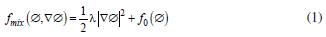
If a double-well potential is used, f₀ is expressed as follows:

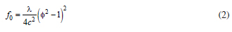
where f₀ is the bulk energy, c is a capillarity width representing the interfacial thickness and λ is the energy density parameter. (Φ) =-1 at liquid region, Φ=1 at gas region and Φ=0 at the interface. The bulk energy shows total separation from the phases in domains of pure components instead of the complete mix of the components. The profile of Φ across the interface is determined by the competition between the two effects. Since the mixing energy represents molecular interaction between the two phases, the interfacial tension is considered equal to the surface tension coefficient σ_T (N/m) which is calculated as follows

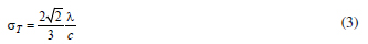
If the interfacial thickness (c) shrinks towards zero, so should the energy density parameter (λ); their ratio gives the interfacial tension in the sharp-interface limit. If the diffuse interface is not at equilibrium but it is relaxing according with the evolution on Equation 6 given below, the interfacial tension is not constant, and in fact it reflects the reality that the interface has its own dynamics which cannot be embodied by a constant interfacial tension except under limiting conditions. The hydrodynamic system describing the mixture of two Newtonian fluids with a free interface can be done with the Navier-Stokes equations and the phase field method. In the solution domains, we consider the continuity and momentum equations in the usual form:

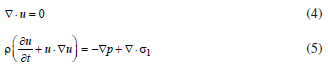
where σ₁ is a deviatoric stress tensor and the field variables, velocity u and pressure p. The surface tension force is added to Navier-Stokes equations as a body force by multiplying the chemical potential of the system by the gradient of the phase field variable (as it is shown in Equation 16). The evolution of the phase field variable is controlled by the Cahn-Hilliard equation.

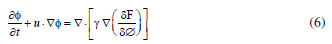
where δF/δΦ = G is the chemical potential (Pa) and g is the mobility (m³ s kg^–1). The mobility determines the time scale of the Cahn-Hilliard diffusion and must be large enough to retain a constant interfacial thickness but small enough so that the convective terms are not overly damped. The mobility is determined by a mobility tuning parameter that is a function of the interface thickness¹⁶.

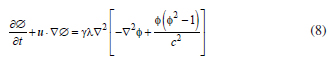
where c is a capillary width that scales with the thickness of the diffuse interface χ (m). The mixing energy considered to produce the interface structure is obtained with Equation 8¹⁶.

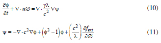
The parameter γλ determines the relaxation time of the interface and it is considered according with Jacqmin²¹. For this case, the two phases have different densities and viscosities; therefore to obtain an incompressible flow solution, the volume of each fluid should remain constant in time. It should not be allowed to change because of diffuse flux. When an amount of fluid 1 flows out of an infinitesimal volume element due to interfacial diffusion, there will be also an amount of fluid 2 of the same volume that would enter the volume element at the same time, and viceversa. To obtain the continuity equation of a divergence-free velocity , a volume average velocity u is defined¹⁶.

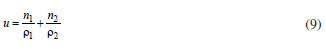
Where n denotes the mass flow rate (per unit volume). Equation 9 represent a mixture of the components by advection without diffusion, thus, the velocity at a special point is defined as that of the component occupying that point; it is spatially continuous and remains solenoidal. The Cahn-Hilliard equation forces the phase field variable (Φ) to take a value of 1 or -1 except in a very thin region on the fluid-fluid interface. The application model decomposes the Cahn-Hilliard equation into two second-order partial differential equations²².

where f_ext is a user defined free energy (J/m³). In this work, the external free energy was zero. In order to model the flow of two different immiscible fluids, a two-phase flow in the phase field method is required. It must be taken into account differences in the two fluids such as densities and viscosities and includes the effect of surface tension and gravity. For this simulation, molten lead and nitrogen gas were considered as fluid 1 and 2, respectively. Therefore, the volume fraction of fluid 2 is computed by the following equation.

The min and max operators are used to consider that the volume fraction has a lower limit of 0 and an upper limit of 1. The density and viscosity are computed by Equation 13 and 14, respectively.

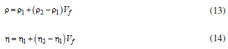
where ρ₁ and ρ₂ are the densities and η₁ and η₂ are the viscosities of fluid 1 and fluid 2, respectively. For incompressible fluids (), in addition of Equations 13 and 14, the Equation 15 was also considered and solved simultaneously with the phase field method.

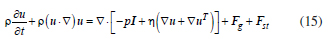
The two forces on the right-hand side of Equation 15 are due to gravity and surface tension. The surface tension and gravity forces are represented in Equation 16 and 17, respectively.

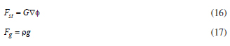
where g is the gravity vector. The mathematical simulation considered the injection of an inert tracer into the molten bath to determine its time dependence. The mixing time is determined from a convection–diffusion model represented by Equation 18.

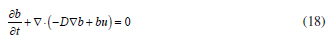
where b is the concentration (kg m^–3), D is the diffusion coefficient (m² s^–1) and u is the velocity (m s^–1). The velocity was obtained from the phase field model solution (Equation 8). The Reynolds number was in the range from 4000 to 26000 for the experimental conditions of this work. Therefore, the laminar diffusion of tracer was excluded due to its low concentration, so the turbulent transport predominate and the diffusion term (D) was obtained from the phase field simulation as a turbulent viscosity (v_T) represented by Equation 19.

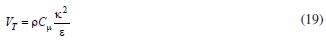
where ρ is the density, C_µ is the turbulence modelling constant (0.09), ε is the turbulent dissipation rate, k is the turbulent kinetic energy²³.

2.2. Numerical solution

Equations given above were solved with the commercial software Comsol Multiphysics 4.1²². The software considers a finite element flow solver that Hu et al.²⁴ have used for simulating particle motion in Newtonian and viscoelastic fluids and an adaptive meshing scheme based in the work of Freitag et al.²⁵. The Cahn Hilliard equation was solved with a combination of the Petrov-Galerkin/Compensated (P-G/C) method²² to discretize spatially to improve stability and the backward difference schemes. P-G/C method uses a modified intrinsic time scale that completely eliminates the streamline diffusion contributions in regions dominated by diffusion. A semi-implicit scheme in which the principal elliptic operator is treated implicitly to reduce the associated stability constraint was used for the time step, while the non-linear terms are still treated explicitly to avoid the expensive process of solving non linear equations at each time step. The accuracy in time can be significantly improved by using higher-order semi-implicit schemes. For this case, a second-order backward difference formula (BDF) was used for the time derivatives and a second order Adams-Bashforth (AB) scheme was used for the explicit treatment of non linear transport terms^18,19. The simulations developed in this work considered grid and time-step refinements to ensure convergence. For the time step, the Courant-Friedricks-Lewy condition (CFL condition) was used^16,26 and it is represented in Equation 20.

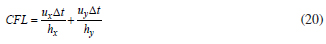
where u is the velocity (m s^–1), ∆t is the time step (s) and h is the length interval (m). For this simulation, a time step such that 2 ≤ CFL ≤ 10 was used to obtain a good relation between efficiency and accuracy. A moderated refined mesh was used to achieve the mass conservation at a discrete level with the finite element method. The phase field theory introduces three model parameters, λ, c, γ which must be pragmatically chosen according to the particular situation to be studied. The simulation must consider the accuracy in the prediction of the interface dynamics and also must preserve the volume of fluids. Yue et al.¹⁷ have validated values of these parameters with an adaptive mesh, which allows handling large interfacial morphological changes.

2.3. Model condition

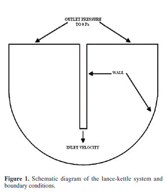
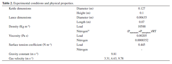
The experimental conditions and the relevant physical data used for the model resolution are given in Table 1. The lance was located at the centerline of the kettle which was symmetrical as can be seen in Figure 1, so the domain solution was represented as a two dimension (2D) slice. The boundary conditions of the kettle contours are shown in Figure 1. The wall in contact with the fluid interface considers a no-slip boundary condition. Therefore, the Equations 21 to 28 were considered.

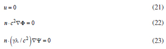
where n is the unit vector normal to the wall. The volume fraction V_f must be specified at the inlet boundaries, normally either 0 or 1.

For outflow boundaries, the following conditions were imposed. During the initialization step, the boundary condition sets the phase field function to 0.

The 2D geometry was meshed in 929 fine triangular elements and 8329 degrees of freedom for greater detail of the phenomena resulting from the simulation. The phase field model allows the use of a fixed Eulerian mesh to capture moving internal boundaries. A mesh with dense grids covering the interfacial region and coarser grids in the bulk are required. As the interface moves out of the fine mesh, the mesh in front needs to be refined while that left behind needs to be coarsened. Such adaptative meshing is achieved by using a general-purpose mesh generator GRUMMP^17,25. The mesh generator provides triangular and tetrahedral elements for 2D and 3D, respectively. The mesh quality is improved through point insertion at the circumcenter of badly shaped cells having and angle smaller than a threshold θ_min. If a proposed new point encroaches on a boundary edge, that vertex is not inserted. Instead, the encroached boundary edge is bisected. This process is repeated until all cells are well shaped. GRUMMP controls the spatial variation of grid size using a length scale (L_s), which specifies the intended grid size at each location in the domain. For this work, the grid size distribution is dictated by the need to resolve thin interfaces. The phase field variable Φ is constant (±1) in the bulk and varies steeply across the interface. A prescribed small grid size h₁ is imposed on the interface by making L_s depend on on every node.

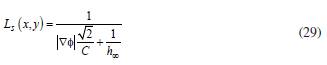
where h_∞ is the mesh size in the bulk, and the constant C controls the mesh size in the interfacial region: being the capillarity width. Values of C between 0.5 and 1 were used to ensure a thickness of the interface to contain the order of 10 grid points. Furthermore, the mesh size can be set to different values for the two bulk fluids.

2.4. Model validation

In order to validate the model results, the residence time was also calculated based on the efficiency of the transitory reaction given by Ohguchi¹³ with the Equation 30 and experimental data reported in the desilvering process during lead refining²⁸.

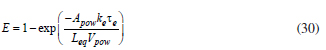
where E is the efficiency of the transitory reaction, A_pow is the particle surface area, k_e is the mass transfer coefficient, t_e is the residence time, L_eq is the equilibrium coefficient of silver concentration in the particle and V_pow is the particle volume. Rearranging terms and solving for the residence time, Equation 30 is represented as follows.

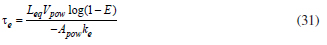
The value of the efficiency of the transitory reaction is in the range from 0 to 1, when E = 1 indicates that the silver particle reacts totally with the molten lead in the residence time. The efficiency of the transitory reaction was considered as 0.25²⁸. The equilibrium coefficient of silver concentration in the particle (L_eq) was obtained with Equation 32.

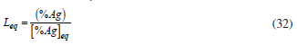
where (%Ag) is the silver particle concentration when it reaches the liquid surface, [%Ag]_eq is the silver content in thermodynamic equilibrium at the process temperature in the bath metal. For this case L_eq was considered in 230.4147 at 480 ºC²⁸. The mass transfer coefficient²⁹ was determined with Equation 33.

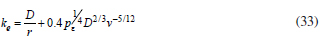
where r is the radius of the particle (m), D is the diffusion coefficient (m² s^–1), pε is the specific mixing power (watt kg^–1) and ν is the kinematic viscosity (m² s^–1). The specific mixing power¹¹ is represented by Equation 34.

where M is the mass of molten metal (kg), Q is the volumetric flow of conveying gas (m³ s^–1), T is the bath temperature (K) and H is the bath depth (m). Substitution of Equations 33 and 34 into 31 gives the residence time. Table 2 shows the parameters considered in the residence time determination calculated with the Ohguchi model.

3. Results

3.1. Gas flow rate

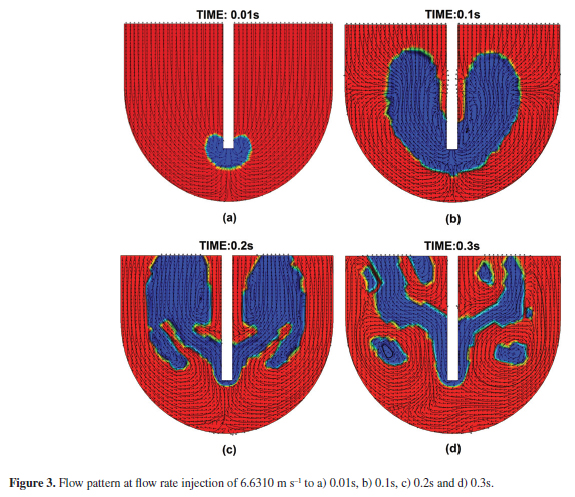
The mathematical simulation was carried out to a flow rate injection of 3.3155, 6.6310 and 9.7887 m s^–1, and it was validated with the results reported by Rodríguez²⁸. The hydrodynamic results are shown in Figures 2, 3 and 4 for a flow rate injection of 3.3155, 6.6310 and 9.7887 m s^–1, respectively for 0.01, 0.1, 0.2 and 0.3 s. The range of time studied in the simulation considers only the effect of the transitory reaction. Figures 2, 3 and 4 presents the flow pattern in the central vertical plane of a lance - kettle symmetrical system in two dimensions. The results of Figures 2 to 4 show the gas bubble formation according to the evolution of the volume fraction of nitrogen gas as time proceeds. The volume fraction of nitrogen gas was increased when time was increased and shows the interfacial layer formed between liquid lead and nitrogen gas which is represented by the phase field variable (Φ) in the Cahn-Hilliard equation. The results show the velocity vectors and black flow lines that indicate the flow trajectory and direction of fluid velocity, as well as a vortex formation zone produced by a metal recirculation flow. This vortex formation was clearly observed located at the central part of the kettle, caused by the rotary motion of molten metal in contact with nitrogen gas. The vortex formation zone was increased when the rate injection was increased. A dead zone formation was observed also at the bottom of the kettle and it was increased to the lower rate injection.

3.2. Residence and mixing time

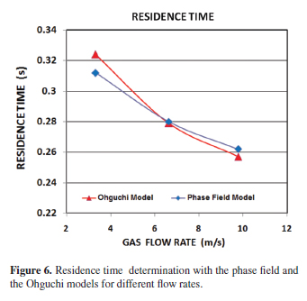
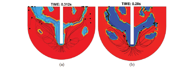
In order to determine the residence time, the partial differential equations were solved time dependent. The residence time indicates the time when the particles are in touch with the liquid metal and therefore represents the time when the transitory reaction is carried out. Figure 5 shows the residence time determination in 0.312, 0.280 and 0.262 s for the injection rate of 3.3155, 6.6310 and 9.7887 m s^–1, respectively. As can be observed, the residence time was decreased when the injection rate was increased. Figure 5 also shows the trajectory of the particle, as can be observed; increasing the gas flow rate increased the injection velocity of the particle and the amount of potential energy dissipated, which contributes to a deeper penetration of the jet. Figure 6 shows the residence time obtained with the Ohguchi model from experimental data and with simulation applying the phase field model. An absolute difference of 0.012, 0.001 and 0.005 s was obtained for both models for the injection rate of 3.3155, 6.6310 and 9.7887 m s^–1, respectively.

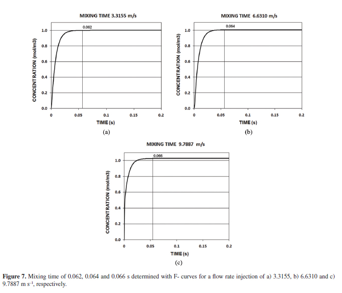
The mathematical simulation considered the injection of an inert tracer into the molten bath to determine its behavior dependent time. The results of these measurements were the F curves shown in Figure 7 for the injection rates considered. The mixing time was determined in 0.062, 0.064 and 0.066 s for the injection rate of 3.3155, 6.6310 and 9.7887 m s^–1, respectively.

3.3. Operating parameters

3.3.1. Lance depth

The effect of the lance depth on the residence and mixing times for the gas flow rate 3.3155 m s^–1 is observed in Figure 8. The lance depth was varied at 30, 50, 70 and 90 % of the kettle height. The results show the velocity vectors and flow lines which indicate the flow trajectory and direction of fluid velocity. Figure 9 shows the results of the mixing and residence time for the three gas flow injections that have been analyzed.

3.3.2. Lance and kettle dimensions

The variation effect of lance and kettle dimensions on the residence and mixing times for the gas flow rate 3.3155 m s^–1 is observed in Figure 10. The lance and kettle measurements reported in Table 1 were affected by a scaling factor to increase and decrease their original dimensions by 50 %. Figure 10 shows the residence and mixing determination times for different lance (Figure 10a) and kettle (Figure 10b) sizes for a flow rate of 3.3155 m s^–1.

4. Discussion

4.1. Gas flow rate

Figures 2, 3 and 4 show that on exit from the lance, at the time of 0.01 s, the nitrogen jet expands rapidly and penetrates only a short distance into the molten lead before rising vertically, at the time of 0.1 s. At this time, the gas plume is almost symmetrical; however, for the times of 0.2 and 0.3 s, the gas plume is not symmetrical, this behavior is due to the internal pressure of the bubble changes as the bubble rises to the surface, as was reported by Kelvin's equation³⁰. P_g = P_l + 2 σ_T/r , where P_g is the pressure inside the gas bubble, P_l is the pressure in the liquid at the level of the bubble, σ_T is the surface tension and r is the radius of curvature. If the super-saturation pressure with respect to the transferred component exceeds P_g, the bubble will grow until it reaches a size where the buoyancy forces exceed the surface tension forces and detachment occurs. It has been reported a transitional range based on Reynolds number³⁰ and modified Froude number³¹, where the bubbles form a continuous jet or discrete bubbles according with the gas flow rate. Generally, the inertial force of gas injected in from the top lance in the low gas flow rate is not strong, therefore there is a forming of discrete bubbles and when the gas flow rate is increased, a continuous jet is promoted, inclusively, a swirl motion on the liquid surface is reached³¹. It was observed the formation of a gas channel during the gas injection instead of the formation of discrete bubbles under all of the simulated conditions. In this work, the effect of the change of pressure in the gas bubble formation was considered in the nitrogen density as is reported in Table 1.

4.2. Residence and mixing time

The residence time represents the time required for the particles leaving the lance tip until they reach the liquid surface supported with the conveying gas. If the residence time decreases, the particles will have less opportunity to react with the liquid bath decreasing the refining metal processes efficiency. Figure 5 shows that when the primary bubble is eliminated by their dissolution on the liquid surface, entrainment of the particle into the plume zone produced by the insoluble gas, resulted in their rapid convection to the upper surface of the bath, where they remained unless the recirculation flow was sufficient to pull them back into the bulk liquid. The vortex formation zone keeps the particle in circulation in the bath when the gas flow rate was increased, as is observed in Figures 5b and 5c. Due to the substantial density difference between the nitrogen gas and the molten lead, the buoyancy force will be dominant enough to assume that the initial velocity of the bubble will be close to final, leaving the particle on the liquid surface. Figure 6 shows the validation of the residence time obtained with Oguchi and phase field models. It must be stressed that the modelling results show ideal conditions of the particular lance-kettle system. Otherwise, Ohguchi's model takes into account an efficiency related with experimental factors such as impurities (Ag, Sb, As, Cu, etc) contained in lead and the temperature control, which directly influences the viscosity of the molten metal and hence the hydrodynamic behavior. However, the differences between both results were considered acceptable for this simulation. The mixing time was obtained to have a better comprehension of the reactor efficiency and hence the process efficiency, considering that the mixing time is an indirect measure of the transfer of momentum from the gas to the liquid³². Figure 7 shows the mixing time determination, which represent the time required to attain a desired level of homogeneity in the bath, this means that in a given time, the concentration in the metal bath is constant.

4.3. Operating parameters

4.3.1. Lance depth

Figure 8 shows that when the lance depth was increased, the volume fraction of nitrogen was increased as well as the molten metal recirculation flow. A metal recirculation flow produced by a vortex formation zone was observed when the lance depth was 70 and 90 %, while a large dead zone was located at the bottom of the kettle to a lance depth of 30 and 50%. Therefore, an increment in lance depth increased, the liquid recirculation velocity and the particle residence time, despite the ensuing increment of recirculation velocity due to the vortex formation. The results of the mixing time show an increase when lance depth was increased; however, an opposite behavior was observed for the gas flow rate of 3.3155 and 6.631 m s^–1 with a lance depth of 30% of the kettle height. This behavior is due to the faster dissipation of potential energy for the cases of lance depths of 30 and 50%, which allows a lower penetration of the jet, as observed in Figures 8a and 8b. A similar behavior was observed when the gas flow rate was increased for the different lance heights in Figure 9.

4.3.2. Lance and kettle dimensions

The results in Figure 10 show that the residence and mixing time were decreased when the lance diameter was increased. Considering that the variation of an average bubble diameter depends on the gas flow and the orifice's diameter, for this case, the gas flow remained constant and the orifice's diameter was modified. Hence, a large area in the lance tip generates a bigger bubble formation. The circulation of gas in a bigger bubble results in the interface movement of the liquid and in a reduction of the drag force on the bubble. Therefore, the buoyancy force is increased, which allows the bubble to rise faster, and to decrease the residence and mixing time. To transfer an adequate momentum and to stir the molten metal in a bigger kettle, an increment in the lance depth¹⁵ or gas flow injection is necessary. A bigger kettle shows an increase in the mixing and residence time for a constant flow rate. A better comprehension of the hydrodynamic behavior of molten metal–gas injection systems will be useful for further studies on the mass transfer of impurity removal on metal refining. The obtained results demonstrate that the injection rate of 3.3155 m s^–1 and the increase of the lance height (deeper position) generate the higher residence and mixing time. This behavior is necessary to obtain an efficient disengagement of the particle from the carrier gas within molten lead. In addition, the kinetic behavior of the particle-metal interaction must be considered as well as operating parameters of the process in order to obtain the highest efficiency in the lead refining process.

5. Conclusions

A mathematical simulation of the operating parameters (lance height, lance and kettle dimensions) was carried out to establish the hydrodynamic behavior in the lance-kettle system for the lead refining process. The residence and mixing time were suitably simulated with the phase-field method and the Cahn Hilliard equation. The effect of gas flow rate, lance depth, and different kettle and lance dimensions were evaluated to obtain the residence and mixing time. The residence and mixing time were decreased when the injection rate and the lance diameter were increased. Therefore, the particle will have less opportunity to react with the liquid bath decreasing the refining metal processes efficiency. When the lance height and kettle dimensions were increased, the residence and mixing time were also increased. The mathematical modelling was validated with the determination of the residence time based on experimental data and Ohguchi's model. The results obtained with both models were similar for the gas flow rate of 3.3155 m s^–1. In order to reach the highest efficiency in lead refining, the residence and mixing time must be considered based on the operating parameters of the process.

Acknowledgements

The authors wish to thank the Institutions SIP-Instituto Politécnico Nacional, CONACyT, SNI and COFAA for their permanent assistance to the Process Metallurgy Group at ESIQIE-Metallurgy and Materials Department.

References

1. Daniel S, Pappis C and Voutsinas T. Applying life cycle inventory to reverse supply chains: a case of study of lead recovery from batteries. Resources Conservation and Recycling. 2003; 37(4):251-281. http://dx.doi.org/10.1016/S0921-3449(02)00070-8

2. Kreusch M, Ponte M, Ponte H, Kaminari N, Marino C and Mymrin V. Technological improvements in automotive battery recycling. Resources Conservation and Recycling. 2007; 52(2):368-380. http://dx.doi.org/10.1016/j.resconrec.2007.05.004

3. Ellis T and Mirza A. The refining of secondary lead for use in advanced lead-acid batteries. Journal of Power Sources. 2010; 195(14):4525-4529. http://dx.doi.org/10.1016/j.jpowsour.2009.12.118

4. Ramachandra S. Resource recovery and recycling from metallurgical wastes. 1th ed. Netherlands: Elsevier; 2006. p. 197-200. Waste Management Series 7.

5. Davey T. The physical chemistry of lead refining: lead-zinc-tin. 1th ed. USA: TMS; 1980. p. 477-507.

6. Hultgren R, Desai D, Hawkins T, Gleiser M and Kelley K. Selected values of the thermodynamic properties of binary alloys. USA: American Society for Metals; 1971. p. 79-121. vol. 2.

7. Charlesworth KJ and Davey TR. The use of METSIM to model multi-stage, desilvering of lead by zinc. In: Extractive Metallurgy of Copper, Nickel and Cobalt, Vol. 1. USA: TMS; 1993. p. 153-167

8. Plascencia G, Romero JA, Morales R, Hallen JM and Chavez JF. Sulfur injection to remove copper from recycled lead. Canadian Metallurgical Quarterly. 2001; 40(3):309-316. http://dx.doi.org/10.1179/cmq.2001.40.3.309

9. Plascencia G. Eliminación de cobre, níquel y plata para el reciclado de baterías. [Thesis]. México: Instituto Politécnico Nacional; 1999.

10. Emi T and Yin H. The Howard Worner International Symposium on Injection in Pyrometallurgy. USA: TMS; 1996. p. 19-38.

11. Vargas M, Romero A, Morales R, Hernandez M, Chavez F and Castro J. Hot metal pretreatment by powder injection of lime-based reagents. Steel Research. 2001; 72(5):173-181.

12. Langberg D and Nilmani M. The injection of solids using a reactive carrier gas. Metallurgical and Materials Transactions B. 1994; 25(5):653-660. http://dx.doi.org/10.1007/BF02655173

13. Ohguchi S and Robertson D. Kinetic model for refining by submerged powder injection. Part 1: transitory and permanent-contact reaction. Ironmaking and Steelmaking. 1984; 11(5):262-273.

14. Schwarz M. Simulation of gas injection into liquid melts. Applied Mathematical Modelling. 1996; 20(1):41-51. http://dx.doi.org/10.1016/0307-904X(95)00109-W

15. Scheepers E, Eksteen J and Aldrich C. Optimization of the lance injection desulphurisation of molten iron using dynamic modeling. Minerals Engineering. 2006; 19(11):1163-1173.

16. Yue P, Feng J, Liu C and Shen J. A diffuse-interface method for simulating two-phase flows of complex fluids. Journal of Fluid Mechanics. 2004; 515:293-317. http://dx.doi.org/10.1017/S0022112004000370

17. Yue P, Zhou C, Feng J, Ollivier C and Hu H. Phase-field simulation of interfacial dynamics in viscoelastic fluid using finite elements with adaptive meshing. Journal of Computational Physics. 2006; 219(1):47-67. http://dx.doi.org/10.1016/j.jcp.2006.03.016

18. Chen L and Shen J. Applications of semi-implicit Fourier- spectral method to phase field equations. Computer Physics Communications. 1998; 108(2-3):147-158. http://dx.doi.org/10.1016/S0010-4655(97)00115-X

19. Liu C and Shen J. A phase field model for the mixture of two incompressible fluids and its approximation by a Fourier-spectral method. Physica D: Nonlinear Phenomena. 2003; 179(3-4):211-228. http://dx.doi.org/10.1016/S0167-2789(03)00030-7

20. Badalassi V, Ceniceros H and Banerjee S. Computation of multiphase systems with phase field model. Journal of Computational Physics. 2003; 190(2):371-397. http://dx.doi.org/10.1016/S0021-9991(03)00280-8

21. Jacqmin D. Calculation of two-phase navier-stokes flows using phase-field modeling. Journal of Computational Physics. 1999; 155(1):96-127. http://dx.doi.org/10.1006/jcph.1999.6332

22. COMSOL Multiphysics 4.1. User's guide CFD module. COMSOL; 2010.

23. Wilcox D. Turbulence modeling for CFD. USA: DCW Industries; 1993. p. 87-89.

24. Hu H, Patankar N and Zhu M. Direct numerical simulations of fluid-solid systems using the arbitrary Lagrangian-Eulerian technique. Journal of Computational Physics. 2001; 1619(2):427-462. http://dx.doi.org/10.1006/jcph.2000.6592

25. Freitag L and Ollivier-Gooch C. Tetrahedral mesh improvement using swapping and smoothing. International Journal for Numerical Methods in Engineering. 1997; 40(21):3979-4002. http://dx.doi.org/10.1002/(SICI)1097-0207(19971115)40:21<3979::AID-NME251>3.0.CO;2-9

26. 26 Courant R, Friedrichs K and Lewy H. On the partial difference equations of mathematical equations. IBM Journal of Research and Development. 1967; 11(2):215-234. http://dx.doi.org/10.1147/rd.112.0215

27. Sokolichin A, Eigenberger G and Lapin A. Simulation of buoyancy driven bubbly flow: established simplifications and open questions. Fluid Mechanics and Transport Phenomena. 2004; 50(1):24-45.

28. Rodríguez JC. Estudio de la eliminación de la plata del plomo líquido mediante la inyección de polvos de zinc. [Thesis]. México: Instituto Politécnico Nacional; 2003.

29. Nilmani M and Langberg D. The production of nickel-zinc alloys by powder injection, metallurgical processes for early twenty-first century. USA: TMS; 1994. p. 653-660.

30. Szekely J. Fluid flow phenomena in metals processing. 1th ed. UK: Academic Press; 1979. p. 462-464.

31. Wang J, Oobayu H, Wang F and Iguchi M. Swirl motion in a cylindrical bath agitated by top lance gas. ISIJ International. 2011; 51(7):1080-1085. http://dx.doi.org/10.2355/isijinternational.51.1080

32. Yong H and Irons G. A water model study of impinging gas jets on liquid surfaces. Metallurgical and Materials Transactions B. 2011; 42(3):575-591. http://dx.doi.org/10.1007/s11663-011-9493-6

Received: September 17, 2013; Revised: May 11, 2014

Publication Dates

• Publication in this collection
  01 July 2014
• Date of issue
  Aug 2014

History

• Accepted
  11 May 2014
• Received
  17 Sept 2013