Urban green spaces and the influence on vehicular traffic noise control

Espaços verdes urbanos e a influência no controle de ruído do tráfego veicular

Abstract

In this paper, we explore a statistical relationship between green areas and traffic-related vehicle noise. A medium-sized Brazilian city was selected as the sampling area. This area was divided into 25 subareas and for each subarea a group of descriptors was developed. The parameters considered were the areas occupied by green spaces and the noise pollution index generated by vehicular traffic during day and night periods. The green areas were quantified by digital processing of satellite images. The vehicular traffic noise was measured directly at the site and analysed by the noise pollution index (L_np), the equivalent sound level (L_Aeq) and the day/night sound level (L_dn). In order to establish the statistical relationship between noise descriptors and green areas, Pearson's linear correlation coefficient (r) was used. Two analysis types were developed: a generalised one, including the 25 subareas; and a specific one, classifying the subareas into clusters. The first analysis indicated a trend to a medium negative correlation between green areas and noise pollution day index (L_npd), noise pollution night index (L_npn) and L_dn (r= -0.577, -0.484, -0.373). In the second analysis, the subarea cluster 3 is considered, which includes areas with clinics and educational institutions. This correlation was classified as high negative (r= -0.729, -0.721, -0.541). The results show indexes with high negative correlation, statistically meaning that there is an inverse proportional relationship between green areas and noise pollution.

Keywords:
Urban green spaces; Noise descriptors; Noise traffic; Acoustic comfort; Satellite images; Image processing

Resumo

Neste trabalho, foi estudada uma relação estatística entre áreas verdes e ruído de tráfego veicular. Uma cidade brasileira de médio porte foi selecionada como área de estudo. Esta área foi dividida em 25 subáreas, e para cada subárea um grupo de descritores foi desenvolvido. Os parâmetros considerados foram as áreas ocupadas pelas zonas verdes e os índices de ruído gerado pelo tráfego veicular em períodos do dia e noite. As áreas verdes foram quantificadas por processamento digital de imagens de satélites. O ruído do tráfego veicular foi medido diretamente no local e analisado pelo índice de poluição sonora (Lnp), o nível de som equivalente (L_Aeq) e o nível de som dia/noite (L_dn). A relação estatística entre descritores de ruído e áreas verdes foi estabelecida usando o coeficiente de correlação linear de Pearson (r). Foram desenvolvidos dois tipos de análise: generalizado, incluindo as 25 subáreas; e específico, classificando as subáreas em clusters. A primeira análise indicou uma tendência para uma correlação negativa média, entre áreas verdes e índice de poluição de ruído diurno (L_npd), índice de poluição de ruído noturno (L_npn) e L_dn (r=-0.577, -0.484, -0.373, respectivamente). Na segunda análise, considera-se o subconjunto 3, que representa áreas com instituições educacionais e clínicas, esta correlação foi classificada como alta negativa (r=-0,729, -0,721, -0,541). Os resultados revelam índices com alta correlação negativa, significando estatisticamente que existe uma relação proporcional inversa entre áreas verdes e poluição sonora.

Palavras-chave:
Espaços verdes urbanos; Descritores de ruído; Ruído de tráfego; Conforto acústico; Imagens de satélite; Processamento de imagens

Introduction

The World Health Organisation (WHO) considers noise pollution as one of the three ecological priorities in the fight against environmental contamination. Noise generated by vehicle traffic increases parallel to motorisation and its effects are now being studied prioritising sectors such as health and transportation (CAI et al., 2017). This noise class is considered to be the greatest generator of acoustic pollution in the urban environment (ASCARIet al., 2015) and it may cause some diseases in the population (ONGEL; SEZGIN, 2016).

Previous studies explored the usefulness of green areas in noise mitigation revealing that:

1. green spaces help minimise factors affecting health, such as traffic noise (PESCHARDT; STIGSDOTTER; SCHIPPERRIJN, 2016);

2. there is noise reduction when restricting vehicle access to parks (COHEN; POTCHTER; SCHNELL, 2014); and

3. vegetation contributes to soundscape perception (BRAMBILLA et al., 2013).

After comparing the acoustic comfort of two squares in the city of Belo Horizonte, Hiroshima and Assis (2017) reported that users are more tolerant to urban noise in the square with most vegetation, where the best ambience and thermal comfort conditions were found. Despite all the efforts and relevant results of these studies, there is still a lack of tools to support the extent of the effect of green areas in controlling noise pollution.

Margaritis and Kang (2016) also relate green areas and some characteristics of urban morphology to traffic noise. Considering eight cities, this analysis included a large number of land use parameters, emphasising the need to combine green areas with areas where there are buildings, roads and demographic attributes to achieve urban noise reduction.

Based on previous experiences that show favourable differences concerning urban noise due to the predominance of green areas, this research describes the contribution of native vegetation to reducing urban noise. In this case, their function as noise barriers was not the main designing purpose of the green areas under consideration. Moreover, other variables may also influence noise propagation. A comparative analysis among noise descriptors is proposed in this paper, highlighting the presence of urban green spaces.

The main component of urban noise and urban vehicular traffic, as well as noise propagation is influenced by many factors (VAN RENTERGHEM; BOTTELDOOREN; VERHEYEN, 2012). Vehicular noise may vary as a function of vehicular speed, driving conditions and vehicular quality. Street intersections and traffic lights may enhance the number of variables in this equation, including: engine speed variation, driver impatience and horn sounds. Other important variables are: air absorption capacity, thermal gradient and street slope. This proposal extracts noise descriptors from direct measurements on site, consequently limiting the expected results in relation to the total control of variables. This limits the scope of our results due to the impossibility of controlling all the variables involved.

This research aims to explore the relationship between green areas and vehicular traffic noise, developing an interdisciplinary proposal. In this approach, artificial vision tools are used to study characteristics of urban environmental and acoustic comfort. Measuring procedures allowed for the construction of sound and green area descriptors, considering 25 subareas within a study area. Two types of quantitative-statistical analyses were considered: a generalised analysis that considers the study area as an integral group and a second analysis that considers some local characteristics to group the subareas into three clusters.

Method

First, the study area was selected. In this area, the city centre was the urban fraction under analysis due to the occurrence of the highest vehicular traffic and the presence of various green areas. For a detailed scale and high analysis resolution, this area was subdivided into sub-areas of equal size. Afterwards, the data were collected. The sound pressure level was measured at a strategically positioned point to analyse each subarea. Within these subareas, the amounts of green areas were calculated by satellite image digital processing. Then, the statistical analyses were carried out.

Delimiting the study area

The study area is located in the central zone of the city of São Carlos in the state of São Paulo - Brazil (Figure 1). São Carlos is a medium-sized city with a population of 243,765 inhabitants (INSTITUTO…, 2016).

Figure 1
The study area in São Carlos central zone, SP, Brazil

The white rectangle in Figure 1 detaches the study area located in the central city zone. All this area is classified as mixed land use area, commercial and residential areas (INSTITUTO…, 2016). The vehicle traffic is constant in this area due to there being a concentration of schools and educational centres, as well as local commerce, tourist sites, squares and parks. Furthermore, there are many trees along the sidewalks.

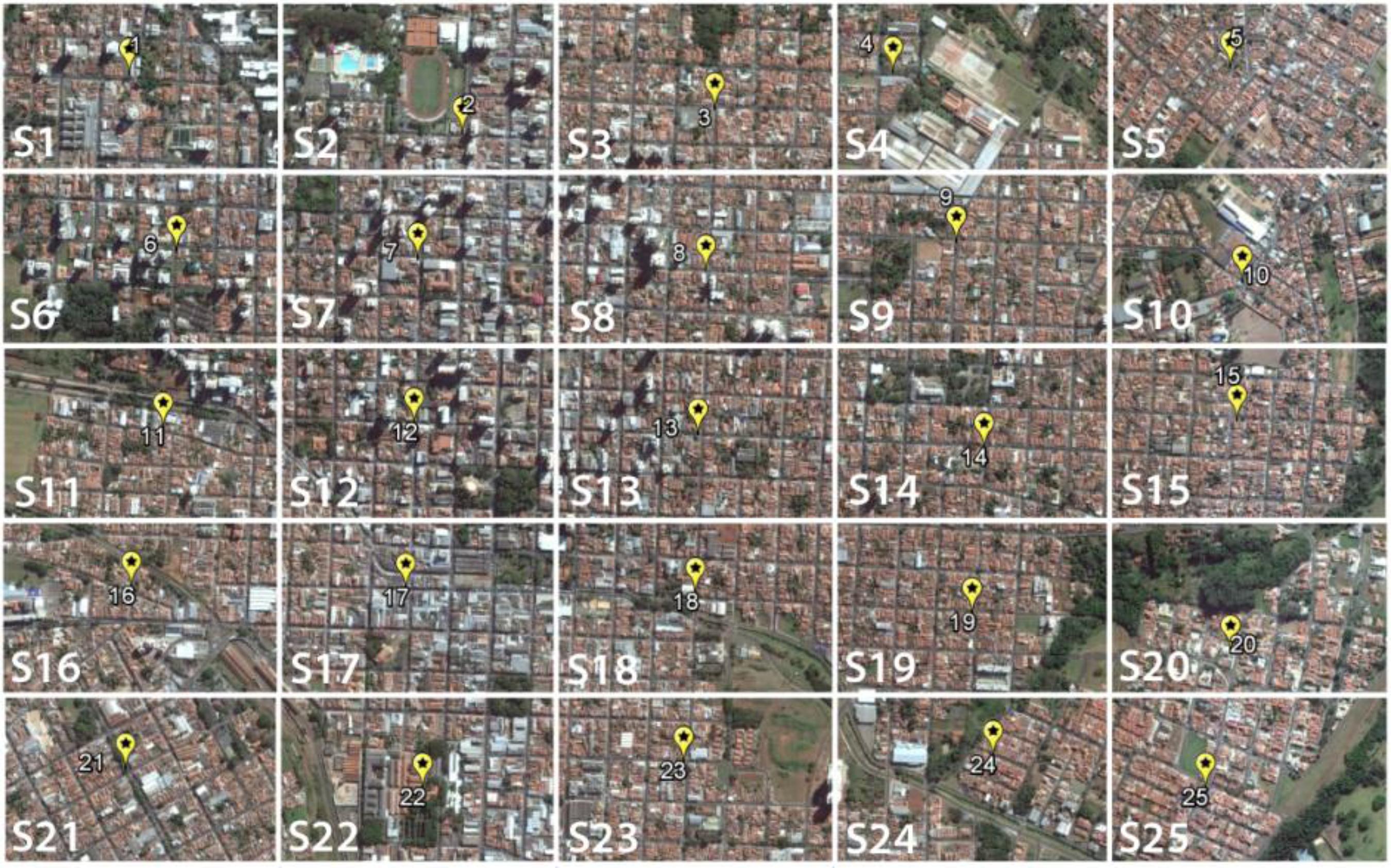
The study area was subdivided into 25 subareas, with uniformly equal dimensions corresponding to 670 m x 375 m. This subdivision was necessary for covering information of the whole central area, while promoting a homogenous distribution of measuring points. Thus, in each subarea a measuring point was placed. Figure 2 shows the division grid adopted to delimit the subareas and collection point locations.

Figure 2
Distribution of the 25 measurement points in the study subareas

Some characteristics sum up other factors influencing the urban noise propagation in the subareas of Figure 2:

1. the subareas S12, S13, S17 and S18 are located in a commercial urban sector, corresponding to the highest commercial concentration;

2. the subareas S4, S5, S10 and S11 present high topographical slopes, corresponding to the highest altitude of the study area;

3. the subareas S2, S3, S6, S9, S10, S12, S14, S17, S22 and S24 include at least one small plaza;

4. the subareas S1, S2, S5, S7, S8, S14 and S20 include educational institutions or medical facilities; and

5. the highest speed limit on the streets of the study area varies between 50 to 60 km/h and their average vehicular traffic is 5.420 (INSTITUTO…, 2016).

Data collection

The data collection followed the procedures by the Technical Standards NBR 10151: Acoustics - Noise Assessment in Inhabited Areas Aiming at the Community’s Comfort fixed by the Brazilian Association of Technical Standards (ABNT, 2000) and the ISO-1996 (MORILLAS; GONZÁLEZ; GOZALO, 2016) fixed by the International Organisation of Standardisation. Thus, the equivalent sound pressure (L_Aeq) measurements were registered with the sound compensation filter A, in decibels dB(A), slow response, in a period of 5 minutes for each measurement. The measurement points kept a distance of 1.2 metres from the ground and at least 2 metres from reflecting surfaces. The limits of the day period extended from 7 am to 10 pm, while the night period corresponded to a period from 10 pm to 7 am of the next day. No measurements were taken under audible interferences of natural phenomena or similar sounds. A Brüel & Kjaer 2270-L sound pressure metre was used for the measurements, and was calibrated and configured according to the aforementioned standards. The vehicular traffic noise was the main sound source under analysis.

Pixel counting determined the green area percentage for each subarea. For this process, a satellite image with a record dated June 21st, 2016 was taken from Google Earth.

Noise descriptors

Two descriptors were used to analyse the noise conditions, the noise pollution index (L_np) and the day/night sound level (L_dn). Equations 1 and 2 show the calculation of the descriptors L_np and L_dn, respectively (BIES; HANSEN, 2009). Values measured at daytime (L_npd) and values at night time (L_npn) were calculated for the L_np descriptor.

Eq. 1 ${\mathit{L}}_{\mathit{np}}={\mathit{L}}_{\mathit{eq}}+\left({\mathit{L}}_{10}-{\mathit{L}}_{90}\right)$

Eq. 2 ${\mathit{L}}_{\mathit{dn}}=10\log \left[\frac{1}{24}\left[15\left({10}^{\frac{{\mathit{L}}_{\mathit{d}}}{10}}\right)+9\left({10}^{\frac{{\mathit{L}}_{\mathit{n}}+10}{10}}\right)\right]\right]$

WhereL_d and L_n correspond to the L_Aeq values of a data collection point, respectively measured at daytime and night time. A night compensation of 10dB was added and was expressed as (L_n + 10).

Determining the green areas percentage

Trees, garden and green covers were considered for counting green areas, while areas only covered by grass were discarded (MARGARITIS; KANG, 2016).

For the subarea pixel counting, the satellite image processing used an adaptation of the Aforapro algorithm (LÓPEZ; KIM, 2014) with the OpenCv and C ++ software. Table 1 presents the steps by which the green areas were counted.

Table 1
Algorithm of the green area parameterisation

Input: size of the green areas in the subareas (x * y) and the entire study area satellite image (I0)

Output: green area value of each subarea (gsi)

1. Satellite image digital processing (I0)

a) Separate the vegetation from other objects using green in the segmentation.

b) Transform the colour image into grey levels

${\mathit{I}}_0\stackrel{\mathit{thresholding}}{\to }{\mathit{I}}_{\mathit{g}}$

c) Exclude grass using the grey intensity differences in the segmentation.

d) Gray image transform to binary image

${\mathit{I}}_{\mathit{g}}\stackrel{\mathit{binaristation}}{\to }{\mathit{I}}_{\mathit{b}}$

Apply black to vegetation and white to complementary areas.

2. Divide study area using the size of the subareas (x + y).

3. Find each subarea coordinates (SAi(xi, yi)) within the binary image (Ib).

4. Count black pixels in each subarea (pci)

${\mathit{SA}}_{\mathit{i}}\left({\mathit{x}}_{\mathit{i}},{\mathit{y}}_{\mathit{i}}\right)\stackrel{\mathit{counts}}{\to }{\mathit{pc}}_{\mathit{i}}$

5. The value of black pixels is equivalent to the value of green areas

${\mathit{pc}}_{\mathit{i}}\to {\mathit{gs}}_{\mathit{i}}$

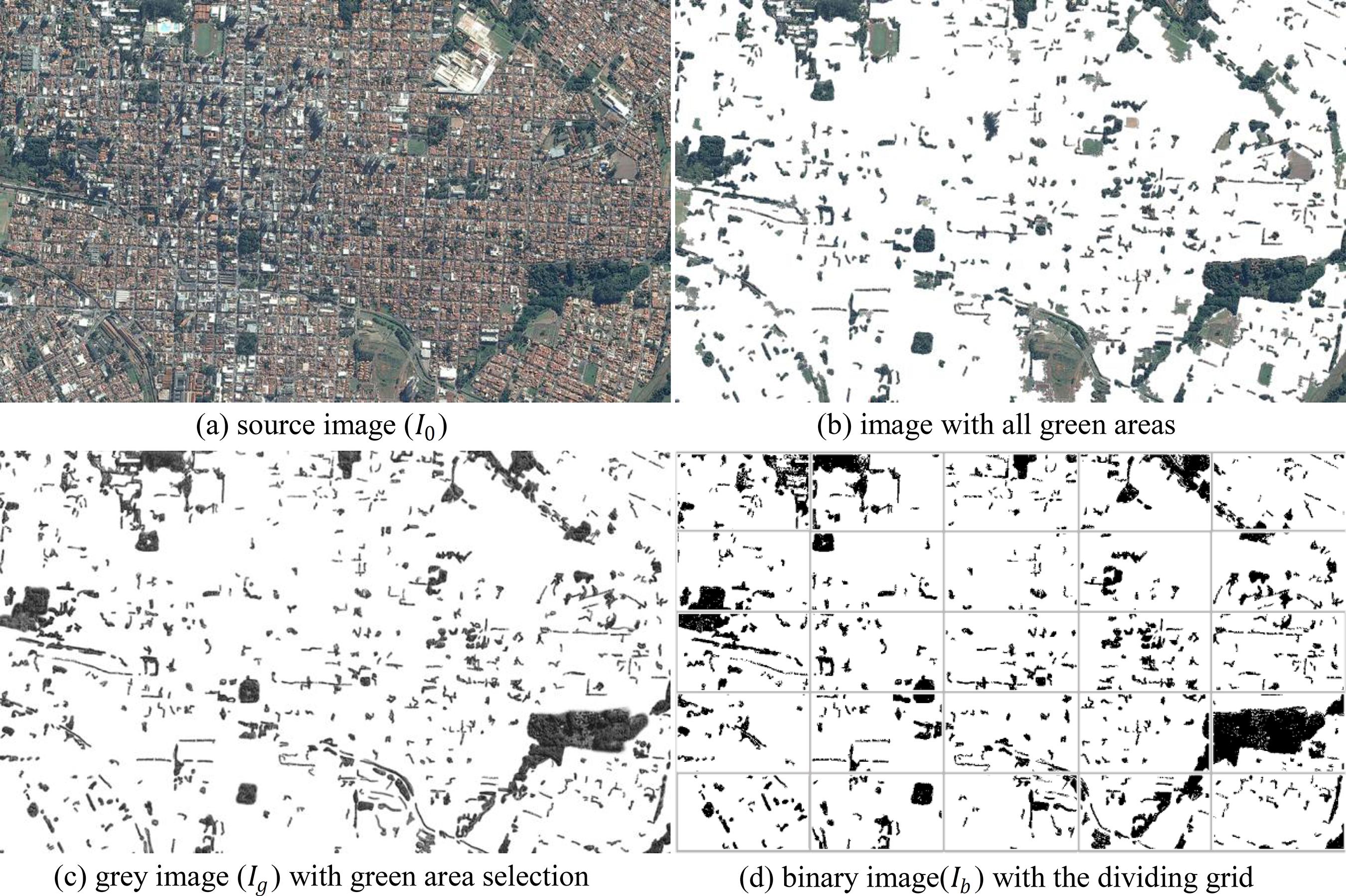
Figure 3 presents four images extracted from some of the digital processing steps.

Figure 3
Study area digital processing for green area parameterisation

Figure 3(a) shows the study area image obtained from Google Earth. In Figure 3(b), the image is filtered using green as a selector. Note that all green coloured areas have been extracted, including some areas of grass. In Figure 3(c), the image is transformed from coloured to grey levels, and is subsequently filtered by intensity values. Note that this second filter eliminates unwanted vegetation. In Figure 3(d), the image is switched from grey levels to two colours (white and black). The division grid was symbolically added to limit the subareas. The pixel counting of each subarea used the image in Figure 3(d).

To classify and extract the green areas, the following resources were used:

1. colouration was able to filter green as a vegetation indicator; and

2. the contrast and tonality of green allowed the classification of low and high size vegetation.

Besides the classifying algorithm configuration, local observations were also made in order to validate the results.

Data analyses

Statistical analyses were used to verify the interrelation between noise and green areas inside the subareas. Three noise descriptors (L_npd, L_npn and L_dn) and a green area descriptor (g_si) were used for each of the 25 subareas. Thus, the behaviour of the noise descriptors was analysed as a function of the green area descriptor variation, and vice-versa.

Two types of analyses were carried out: a generalised analysis, which considers the subareas as an integral set; and a specific analysis, which divides the subareas into three clusters.

A database containing the characteristics of each subarea was created, and then, using the k-means algorithm, the subareas were classified into clusters. This classification obtained the specificity of each area for the analysis. The local characteristics considered were: low vegetation, houses with up to two floors, tall buildings (more than two floors), number of commercial stores, buildings with terrace/pool or garden, educational institutions, number of squares or parks, and percentage of non-built areas. The three largest clusters were selected by considering the number of subareas included. The following clusters were determined: Class 1 - subareas with high percentage of low vegetation; Class 2 - subareas with high building predominance; and Class 3 - subareas with the presence of educational buildings and health facilities. Table 2 shows a comparative table of the level of influence between the three classes determined.

Table 2
Characteristics influencing the acoustic behaviour of each class

Characteristic	Influence level
	Class 1	Class 2	Class 3
Facade of the buildings acting as acoustic barriers: they reduce the noise to the interior and reflect to the sidewalk	very low	very high	moderate
People´s intermittent focus and concentration: increases vehicular mobility	very low	moderate	very high
Effect of soil covered by pavement: influence the emission of noise by friction and reflection	very low	high	very high

Results: the noise descriptors and parameters

This section initially presents the measured and calculated values for the noise descriptors and for the green area parameters, as well as their distribution. Subsequently, the following two analyses are presented: by each sub-area and by clustered sub-areas.

The subarea descriptors and parameters

Table 3 shows the 25 subareas (Figure 2), indicating the number of pixels counted as green areas, the equivalent percentage of the green area inside the subarea (for a total of 836148 pixels), and the noise descriptors for daytime and night time periods (L_Aeq, L₁₀ and L₉₀).

Table 3
Values of Noise descriptors and green areas

Points	Green area			Noise Descriptors
				Day			Night
	(pixels)	(%)	*R1	Leq(A)	L90	L10	Leq(A)	L90	L10
s1	208659	24.96	0.33	54.11	39.93	58.88	59.37	50.53	62.47
s2	209062	25.01	0.33	55.64	46.01	58.25	56.34	50.84	59.04
s3	134079	16.04	0.19	68.35	61.18	69.97	59.07	49.03	62.04
s4	216578	25.91	0.35	66.05	53.48	68.54	64.09	49.66	63.69
s5	100349	12.01	0.14	72.03	55.97	73.58	71.39	57.98	76.06
s6	136569	16.34	0.20	65.15	50.69	66.53	68.19	57.59	69.44
s7	80123	9.59	0.11	68.22	55.26	70.90	69.74	56.10	72.62
s8	53192	6.37	0.07	71.53	59.17	73.13	70.02	54.89	73.39
s9	79905	9.56	0.11	68.78	51.59	69.61	68.22	52.68	71.40
s10	144420	17.28	0.21	71.55	63.30	73.48	70.21	61.64	72.20
s11	213646	25.56	0.34	64.98	57.32	67.71	64.10	56.44	65.22
s12	103201	12.35	0.14	66.63	59.26	69.67	65.00	54.36	64.35
s13	99371	11.89	0.13	68.47	54.25	70.93	71.03	58.05	72.20
s14	138058	16.52	0.20	76.45	63.58	77.55	68.68	48.37	68.56
s15	119167	14.26	0.17	59.20	44.96	62.57	61.21	47.70	63.36
s16	96852	11.59	0.13	63.23	49.60	67.04	64.74	52.19	67.81
s17	138683	16.59	0.20	65.24	47.48	69.23	65.69	50.77	68.46
s18	109212	13.07	0.15	65.83	56.40	69.52	60.32	51.43	63.02
s19	110255	13.19	0.15	66.74	48.45	70.16	65.78	53.55	67.79
s20	403370	48.25	0.93	56.04	41.40	57.03	64.54	57.56	64.67
s21	94951	11.36	0.13	63.51	54.11	66.33	61.20	52.51	63.97
s22	132305	15.83	0.19	72.28	61.68	74.88	62.89	49.06	62.66
s23	103957	12.44	0.14	67.36	54.31	71.18	60.39	51.79	63.15
s24	227781	27.25	0.37	66.86	60.94	69.09	56.18	53.86	58.52
s25	121391	14.52	0.17	65.92	58.21	68.34	57.94	52.97	59.49

• Nota:
• ^*
  R1 is the relationship between the built area and green spaces area percentage.

Each subarea has a significant component of green areas, ranging from 6.37% to 27.25%, with only one subarea presenting a value outside this range and reaching 48.25% (subarea 20).

The nocturnal environment, in some cases, presents less background noise - for instance, in the case of subarea s14 (63.58 dB(A), 48.37 dB(A)) and s22 (61.68 dB(A), 49.06 dB(A)). However, other examples demonstrate the contrary, as observed in subareas s1 (39.93 dB(A), 50.53 dB(A)) and s20 (41.40 dB(A), 57.56 dB(A)). As expected, due to the lower number of nocturnal noise sources, the mean value of peak-noise is higher during the day (69.52dB(A)) than during the night (64.57dB(A)). In general, the mean value of daytime L_Aeq (66.63dB(A)) is slightly higher than the nocturnal value (64.54dB(A)). These variations in the data highlight the potential for the analysis proposed here.

The ratio between the percentage of constructed area and the green area (R1 = % green area/(100 - (% green area))) shows the influence of the green areas on the vehicular noise. The subarea s20, which has a R1_max(0.93), is coincident to the lowest noise ranges of the descriptors. While the subarea s8, which corresponds to R1_mix(0.07), presents the highest noise ranges of the descriptors. Other subareas may also exemplify this tendency, for instance: subarea s5 presents one of the lowest values of R1(0.14) and the highest values of nocturnal noise Leq(A)_max (71.39) and L10_max(76.06), while subarea s1 shows one of the highest values ofR1(0.33) and presents the lowest daily noise Leq(A)_min (54.11) e L90_min (39.33).

Distribution of noise descriptors and green areas

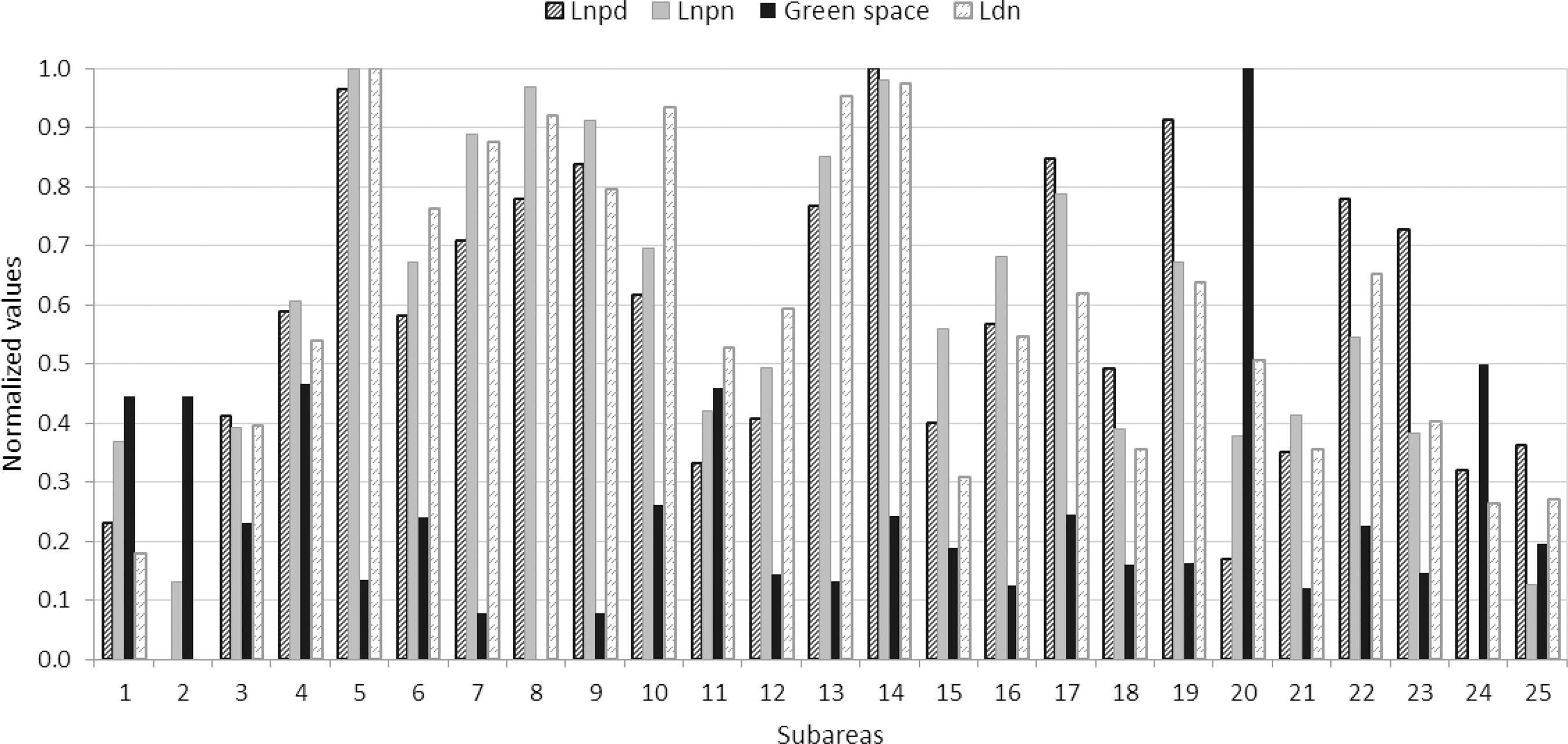
To verify the descriptor distribution together with the green areas, the pixel quantities were normalised (in the interval from 0 to 1), respectively corresponding to the lowest and highest values, 6.37% and 48.25%). This distribution is represented in Figure 4.

Figure 4
The noise descriptors and green area distribution (normalised values [0, 1])

Note that in subareas s5, s7, s8, s9, s13 and s14, some of the highest noise descriptor values coincide with the amount of low green space. In contrast, in subareas s20 and s24, some of the smallest noise descriptor values coincide with the largest green area values. Thus, this distribution analysis reveals a tendency in the relationship between the noise level and the amount of green areas.

Green areas and sound pollution index (L_np)

The daytime and night-time noise pollution indices (L_npd and L_npn) and their relationship to the green areas, as highlighted in Figure 5, were observed. For the analysis of this figure, the subareas represented in the X axis do not follow the numerical sequential order (s1, s2, s3 ... to s25) as they were organised to obtain an upward variation of the green area values.

Figure 5
Relationship between green areas and L_npd and L_npn

The percentage of green areas ranges from 6.37% to 48.27%, the L_npd from 55.64 dB(A) to 76.45 dB(A) and the L_npn from 56.18 dB(A) to 71.39 dB(A). The noise descriptor values alternate between increasing and decreasing patterns for small increases in green area percentages up to the point where the normalised value of 0.24 (corresponding to 16.59%) is reached. However, above this value, there is a strong transition from L_np to lower levels, which coincides with the increasing percentage of green areas.

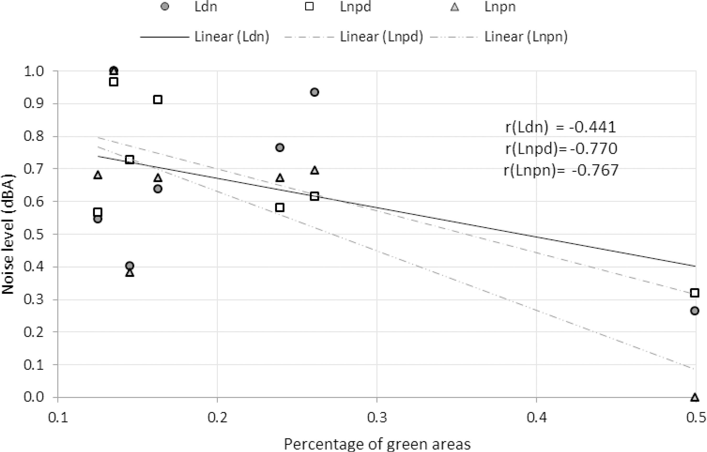
Applying the Pearson (r) linear correlation coefficient for a statistical analysis of the relationship between two variables, three classes can be considered: High correlation if r ∈ abs[0.5, 1.0], medium correlation if r ∈ abs[0.3, 0.5] or low correlation r ∈ abs[0.1, 0.3]. The correlation can also be positive or negative: a positive correlation indicates a contrast between high-high values, while a negative one indicates a contrast between high-low values (BENESTY et al., 2009).

The graph (Figure 6) indicates the values r(L_npd) = -0.577 and r(L_npd) = -0.484 representing a high correlation for the first value and a medium correlation for the second one. The negative sign in the values means that when the percentage of green spaces increases, the values of L_np decrease or vice versa.

Figure 6
Correlation between green areas and sound pollution index

Green spaces and day-night sound levels (L_dn)

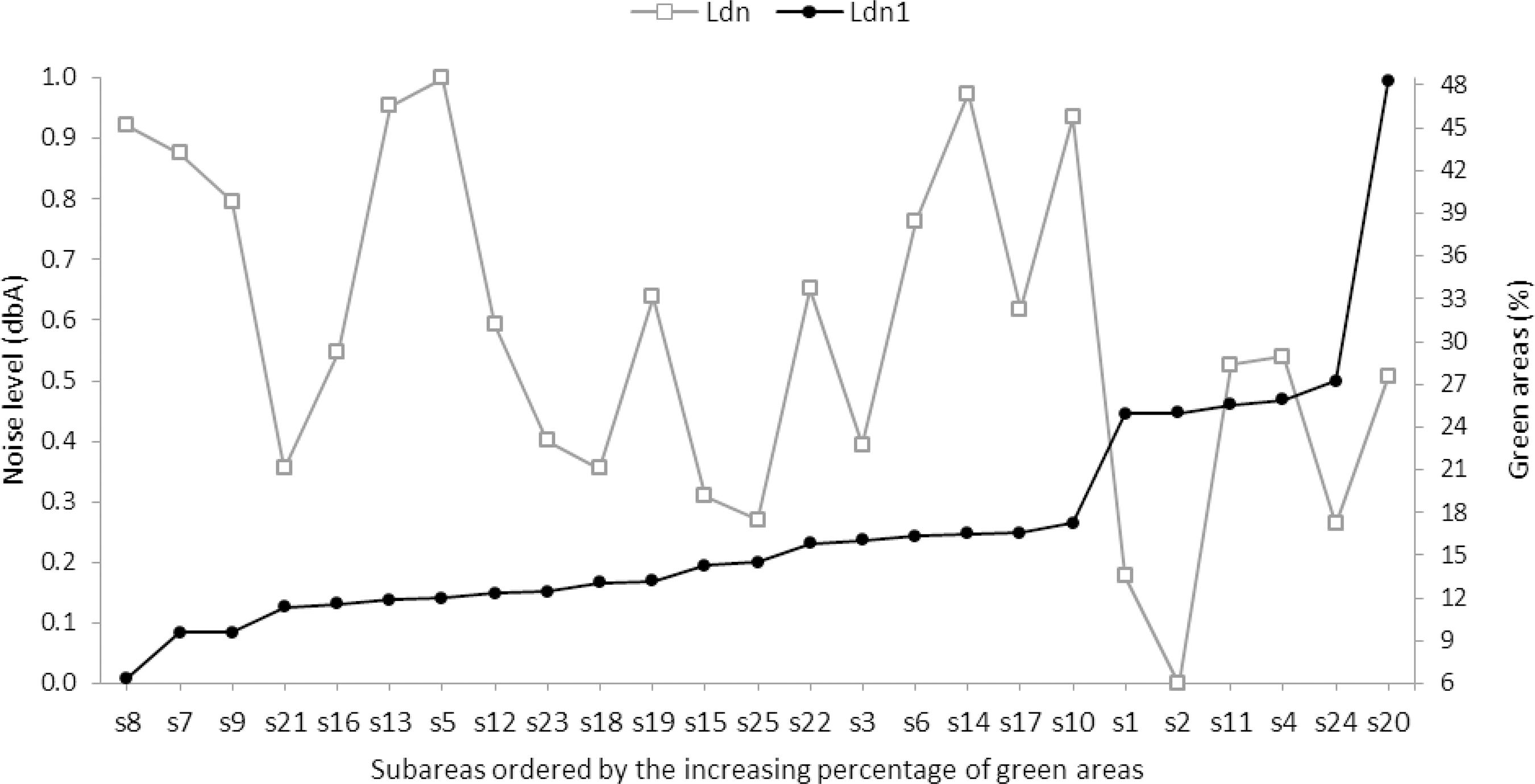
The green areas and L_dn distribution are shown in Figure 7, in which the subareas also appear in increasing order according to the percentage of green areas.

Figure 7
Relationship between green areas and L_dn

The L_dn values ranged from 62.7 dB(A) to 77.9 dB(A). The decrease in the L_dn descriptor value for the subareas with more green areas is not as significant as the one presented previously by the L_np descriptors. However, the L_dn descriptor presents high values for subareas s8 (L_dn value 0.92), s13 (L_dn value 0.95) and s5 (L_dn value 1.00), which coincide with the lowest values percentages of green area components (6.37%, 11.89%, 12.1%). In contrast, L_dn presents low values in subareas s2, s20 and s24 (values of 0.00, 0.50 and 0.26, respectively), which coincide with high values of green areas (25.01%, 48.25% and 27.25%, respectively). Thus, the L_dn distribution graph also shows a significant relationship between green areas and L_dn.Figure 8 represents the correlation analysis between green areas and L_dn, in which a linear correlation with a negative slope is observed.

Figure 8
Relationship between green areas and the day-night sound level

In this case, the Pearson coefficient (r = -0.373) expresses medium correlation between these two variables. This coefficient reached a lower value than the L_np coefficient, indicating less significant correlation between the variables of L_dn and the percentage of green areas.

Analysis for clustered subareas

In this analysis, the subareas are divided into three clusters or classes and each class includes seven subareas. Some subareas may be present in more than one cluster because the classes are not mutually exclusive. As mentioned before, the Pearson coefficient (r) is used to analyse the linear correlation between the sub-area classes and the descriptors.

Class 1 cluster: high percentage of low vegetation

This class includes areas whose vegetation height is less than or equal to 50 cm. The range of values presented by the percentage of green areas in this cluster ranged from 14.2% to 37.5%. Table 4 shows the normalised values for the noise descriptors and the percentage of green areas presented by this class 1 cluster. Figure 9 shows the linear correlation graph between the descriptors and the class 1 subareas.

Table 4
Class 1 normalised values

Subareas	green areas	Ldn	Lnpd	Lnpn
s5	0.135	1.000	0.965	1.000
s6	0.239	0.763	0.580	0.672
s10	0.261	0.934	0.616	0.696
s19	0.163	0.638	0.912	0.672
s23	0.145	0.4014	0.726	0.382
s24	0.499	0.263	0.319	0.000
s25	0.195	0.2698	0.363	0.126

Figure 9
Relationship between Class 1 cluster and descriptors

This class of subareas showed a high correlation with L_npd (r = -0.715) and with L_npn (r = -0.610), although it presented a medium correlation with L_dn (r = -0.394). Compared with the generalised analysis, there was an increase in the correlation coefficient (-0.577, -0.484, -0.373), which indicates that the percentage of low vegetation strengthens the correlation between green areas and noise descriptors.

Class 2 cluster: predominance of high buildings

This class includes areas with tall buildings (more than two floors). In the subareas s7, s8, s9 and s12 (Table 5), most buildings are for commercial purposes. In the subareas s6 and s13, there is a majority of industrial buildings. In subarea s22, there are mostly residential buildings. Figure 10 presents the linear regression between class-2 and the descriptors.

Table 5
Class-2 normalised values

Subareas	Green areas	Ldn	Lnpd	Lnpn
s6	0.239	0.763	0.580	0.672
s9	0.077	0.875	0.708	0.889
s8	0.000	0.921	0.779	0.969
s7	0.077	0.796	0.837	0.913
s12	0.143	0.592	0.408	0.494
s13	0.132	0.954	0.766	0.850
s22	0.226	0.651	0.779	0.546

Figure 10
Relationship between Class-2 cluster and descriptors

The Pearson coefficient indicates a medium correlation for L_npd (r = -0.335), while for L_npn (r = -0.776) and L_dn (r = -0.580), there was a high correlation. Comparing them to the generalised analysis coefficients (-0.577, -0.484, -0.373), respectively, there was a reduction for L_npd and a significant increase for L_npn and L_dn.

In Table 5, it can be observed that there was a high contrast between low green area values and high noise descriptor values for the subareas s7, s8, s9 and s13. This contrast increases the negative linear correlation. However, all green area values are low, which makes the opposite effect difficult to identify - i.e. what would happen under conditions of high green area values. On the other hand, most buildings in subareas s7, s8 and s9 are for commercial purposes, which may indicate that areas with commercial buildings need to increase green areas to improve sound pollution control.

Class 3 cluster: presence of educational buildings and health facilities

The areas that have health facilities and educational institutions have a different dynamic due to the concentration of human activities and population mobility. Each subarea of this class has at least one clinic and/or educational institution. In this class 3 cluster, there are two subareas with extreme values of green area percentages: s8 and s20 (Table 6). Figure 11 shows the linear regression analysis for this cluster.

Table 6
Class 3 normalised values

Subareas	N. green space	Ldn	Lnpd	Lnpn
s1	0.444	0.178	0.231	0.368
s2	0.446	0.000	0.000	0.130
s5	0.135	1.000	0.965	1.000
s7	0.077	0.796	0.837	0.913
s8	0.000	0.921	0.779	0.969
s14	0.243	0.974	1.000	0.980
s20	1.000	0.507	0.169	0.378

Figure 11
Class-3 correlation descriptors

The Pearson coefficients for L_npd (r = -0.729), L_npn (r = -0.721) and L_dn (r = -0.541) indicate high correlation between green area percentages and noise descriptors. These results are even more significant than those obtained for the analysis of class-1 and class-2, because in this case the variations in the green area percentage are almost equidistant and include the extreme values (minimum and maximum scale values). Therefore, the contrast of the descriptors influenced by the variety of values can be observed. Thus, Figure 10 and Table 5 show that for the smallest green area percentage of s8 (0.000), noise descriptor values are high (L_npd = 0.921, L_npn = 0.779 and L_dn = 0.969). The response is inverse in s20 (1.000), for which the highest green area percentage corresponds to relatively low noise descriptor values (L_npd = 0.507, L_npn = 0.169 and L_dn = 0.378).

Discussion

Historically, environmental health organisms have focused on the combat of water and air contamination. However, nowadays the noise pollution has been also included by the World Health Organisation as a public health problem.

According to Babisch et al. (2005), sound levels above 55 dB(A) are considered alarming noises because of the annoyance caused on the hearing comfort. Chronic exposition to noises ranging from 65 to 80 dB(A) may cause damage to the hearing function. The same authors also indicate that the most prominent common kind of urban noise pollution is vehicular traffic noise, which may cause physiological and cognitive changes, sleep disturbance and psychosocial stress. Ascari et al. (2015) comment that in the European Union more than 40% of the population are exposed to vehicular traffic noise above 55 dB(A) and 20% to levels above 65 dB(A).

Noise levels registered in the city of São Carlos (SP), the study area of this research, range from 55.64 dB(A) to 76.45 dB(A) during the day and from 56.18 dB(A) to 71.39 dB(A) during the night, which are alarming ranges for a medium sized city. The urgency for advances considering the management of urban noises is clear.

Acoustical mapping of cities is one of the first steps in this direction. The acoustic map is an instrument of sustainable development, which may give a fundamental basis for the acoustical health analysis of a city. This tool may be used by urban technicians, decision makers, urban planners, control organisms or citizens.

The European Parliament, by means of the European Directive, defined in 2002 a plan action and guide for the combat of noise pollution. In the United States of America, the Environmental Protection Agency investigates noise and its effects, disseminates information about urban noise and evaluates the effectiveness of rules for health protection and public well-being. In Latin America, many cities have already started using noise maps, as in the case of Santiago in Chile, Bogotá in Colombia, Buenos Aires in Argentina and Fortaleza in Brazil.

Vegetation is considered a cheap and natural material to reduce noise pollution in open spaces compared to concrete, metal, plastic or other artificial materials (YANG; BAO; ZHU, 2011). According to Van Renterghem, Botteldooren and Verheyen (2012), there are three main effects of green areas that cause reduction on noise pollution: diffraction and reflection of sound waves by the vegetated elements, absorption of sound waves and transformation in mechanical vibrations, and destructive interference of sound waves.

Some prediction methods of vehicular traffic noise also take into account the vegetation effect on sound propagation. For instance, considering the algorithm of ISO 9613-2 (VAN; VERHEIJ, 2017) dense foliage is incorporated in the FHWA model, in the Nord2000 Road model, “dispersion zones” or vegetation is considered in relation to the density, diameter and absorption coefficient of the tree.

In the first general analysis, in which the study area was considered as an integral group, the results show that the distribution of green areas in the urban fabric could reduce the traffic noise. Moudon (2009) agrees with this statement and highlights that green spaces are useful in noise attenuation due to three factors: their physical characteristics, the restriction to a high concentration of population and car use restriction. In addition, Margaritis and Kang (2016) believe that the dispersion of green areas combined with the properties and attributes of roads and buildings are factors that considerably reduce noise levels.

The general analysis helped confirm this influence, at least for the three descriptors under evaluation (L_npd, L_npn, L_dn), although showing that only a slight tendency of low descriptor values are related to a high percentage of green areas. However, due to the multitude of variables influencing the subareas, this relationship was not so clear.

Therefore, the cluster analysis has become more useful, clarifying this relationship. When the subareas were divided into groups, there was often an increase in the correlation between subareas and noise descriptors. Consequently, the results show that the correlation coefficient between green areas and noise pollution may vary according to the characteristics of the subareas. The cluster presenting the most attenuating effect of the green areas was class 3, where there are a greater number of health facilities and educational buildings. This effect may be related to the particular concentration of activities occurring in this area, which increases road traffic and the number of sound sources (KINDA; LE COURTOIS; STÉPHAN, 2017; SAKIEHet al., 2017).

Thus, valorisation and/or inclusion of green spaces in the urban fabric should be a strategic action in cities' policies (RICHARDSON; MITCHELL, 2010; CURRIE, 2017).

Conclusion

Considering the vehicle traffic as the main source of noise and by using the linear coefficient of Pearson (r) as a statistical parameter, some statistical relationships between green spaces and some sound descriptors, such as the L_npd, L_npn, and L_dn, were established. After developing two types of analyses, different levels of information could be extracted. For the general analysis, in which the study area was divided into 25 subareas, the coefficients pointed out a tendency of a medium negative correlation. For the other analysis, in which the study area was grouped into three clusters, the calculated coefficients showed a high negative correlation.

The conclusion of the data analysis and the literature review is that vegetation presents a potential to attenuate urban noise. For the case of São Carlos, we estimate that a green area with native specimens may mitigate 3 to 5 dB(A) in noise levels.

The results present important generalisations, useful for urban planning purposes and for the acoustical evaluation of the presence of vegetation on the city. This research also helps advances of noise evaluation procedures and the acoustical technical basis for the proposition of urban green areas.

The results of this research are limited to the study of the influence of green spaces on urban noise control. Other factors such as topography, building geometry or surface materials were not taken into account and may have probably also contributed to the urban noise heterogeneous reduction identified in each analysed subarea.

Acknowledgments

This research was supported by Coordination for the Improvement of Higher Education Personnel (CAPES).

References

• ASCARI, E. et al Low Frequency Noise Impact From Road Traffic According to Different Noise Prediction Methods. Science of the Total Environment, v. 505, p. 658-669, 2015.
• ASSOCIAÇÃO BRASILEIRA DE NORMAS TÉCNICAS. NBR 10151: acústica: avaliação do ruído em áreas habitadas, visando o conforto da comunidade. Rio de Janeiro, 2000.
• BABISCH, W. et al Traffic Noise and Risk of Myocardial Infarction. Epidemiology, v. 16, p. 33-40, 2005.
• BENESTY, J. et al Pearson Correlation Coefficient. In: COHEN, I. et al Noise Reduction in Speech Processing Heidelberg: Springer, 2009.
• BIES, D. A.; HANSEN, C. H. Engineering Noise Control: theory and practice.Boca Ratón: CRC press, 2009.
• BRAMBILLA, G. et al The Perceived Quality of Soundscape in Three Urban Parks in Rome. The Journal of the Acoustical Society of America, v. 134, n. 1, p. 832-839, 2013.
• CAI, Y. et al Long-Term Exposure to Road Traffic Noise, Ambient Air Pollution, and Cardiovascular Risk Factors in the HUNT and Lifelines Cohorts. European Heart Journal, v. 38, n. 29, p. 2290-2296, 2017.
• COHEN, P.; POTCHTER, O.; SCHNELL, I. A Methodological Approach to the Environmental Quantitative Assessment of Urban Parks. Applied geography, v. 48, p. 87-101, 2014.
• CURRIE, M. A. A Design Framework For Small Parks in Ultra-Urban, Metropolitan, Suburban and Small Town Settings. Journal of Urban Design, v. 22, n. 1, p. 76-95, 2017.
• HIROSHIMA, S. Q. da S.; ASSIS, E. S. de. Percepção Sonora e Conforto Acústico em Espaços Urbanos do Município de Belo Horizonte, MG. Ambiente Construído, Porto Alegre, v. 17, n.1, p. 7-22, jan./mar. 2017.
• INSTITUTO BRASILEIRO DE GEOGRAFIA E ESTATÍSTICA. Censo Demográfico, 2010 Available: <www.ibge.gov.br>. Accessed: Sep. 14, 2016.
  » www.ibge.gov.br
• KINDA, G. B.; LE COURTOIS, F.; STÉPHAN, Y. Ambient Noise Dynamics in a Heavy Shipping Area. Marine Pollution Bulletin, v. 124, n. 1, p. 535-546, 2017.
• LÓPEZ, G. A. P.; KIM, H. Y. Comparison of Viewpoint-Invariant Template Matchings. In: Telecommunications Symposium (ITS), 2014. Proceedings… IEEE, 2014.
• MARGARITIS, E.; KANG, J. Relationship Between Urban Green Spaces and Other Features of Urban Morphology With Traffic Noise Distribution. Urban Forestry & Urban Greening, v. 15, p. 174-185, 2016.
• MORILLAS, J.; GONZÁLEZ, D.; GOZALO, G. A Review of the Measurement Procedure of the ISO 1996 Standard: relationship with the European Noise Directive. Science of the Total Environment, v. 565, p. 595-606, 2016.
• MOUDON, A. V. Real Noise From the Urban Environment: how ambient community noise affects health and what can be done about it. American journal of preventive medicine, v. 37, n. 2, p. 167-171, 2009.
• ONGEL, A.; SEZGIN, F. Assessing the Effects of Noise Abatement Measures on Health Risks: a case study in Istanbul. Environmental Impact Assessment Review, v. 56, p. 180-187, 2016.
• PESCHARDT, K. K.; STIGSDOTTER, U. K.; SCHIPPERRIJN, J. Identifying Features of Pocket Parks That May be Related to Health Promoting Use. Landscape Research, v. 41, n. 1, p. 79-94, 2016.
• RICHARDSON, E. A.; MITCHELL, R. Gender Differences in Relationships Between Urban Green Space and Health in the United Kingdom. Social science & medicine, v. 71, n. 3, p. 568-575, 2010.
• SAKIEH, Y.et al Green and calm: modeling the relationships between noise pollution propagation and spatial patterns of urban structures and green covers. Urban Forestry & Urban Greening, v. 24, p. 195-211, 2017.
• VAN RENTERGHEM, T.; BOTTELDOOREN, D.; VERHEYEN, K. Road Traffic Noise Shielding by Vegetation Belts of Limited Depth. Journal of Sound and Vibration, v. 331, n. 10, p. 2404-2425, 2012.
• VAN, B.; VERHEIJ, T. Quality Assured Implementation of ISO 9613 in Software.Proceedings of ACOUSTICS, v. 19, n. 22, 2017.
• YANG, F.; BAO, Z.; ZHU, Z. An Assessment of Psychological Noise Reduction by Landscape plants. International Journal Environ Res Public Health, v. 8, p. 1032-1048, 2011.

Publication Dates

• Publication in this collection
  Oct-Dec 2018

History

• Received
  18 Nov 2017
• Accepted
  23 Feb 2018