A shell finite element formulation to analyze highly deformable rubber-like materials

A shell finite element formulation to analyze highly deformable rubber-like materials

J. P. Pascon^*; H. B. Coda

Department of Structural Engineering, São Carlos School of Engineering, University of São Paulo, São Carlos, São Paulo, Brazil

ABSTRACT

Abstract: In this paper, a shell finite element formulation to analyze highly deformable shell structures composed of homogeneous rubber-like materials is presented. The element is a triangular shell of any-order with seven nodal parameters. The shell kinematics is based on geometrically exact Lagrangian description and on the Reissner-Mindlin hypothesis. The finite element can represent thickness stretch and, due to the seventh nodal parameter, linear strain through the thickness direction, which avoids Poisson locking. Other types of locking are eliminated via high-order approximations and mesh refinement. To deal with high-order approximations, a numerical strategy is developed to automatically calculate the shape functions. In the present study, the positional version of the Finite Element Method (FEM) is employed. In this case, nodal positions and unconstrained vectors are the current kinematic variables, instead of displacements and rotations. To model near-incompressible materials under finite elastic strains, which is the case of rubber-like materials, three nonlinear and isotropic hyperelastic laws are adopted. In order to validate the proposed finite element formulation, some benchmark problems with materials under large deformations have been numerically analyzed, as the Cook's membrane, the spherical shell and the pinched cylinder. The results show that the mesh refinement increases the accuracy of solutions, high-order Lagrangian interpolation functions mitigate general locking problems, and the seventh nodal parameter must be used in bending-dominated problems in order to avoid Poisson locking.

Keywords: large deformation analysis; homogeneous rubber-like materials; shell finite elements.

1 INTRODUCTION

Highly deformable elastic shell structures have been widely used in engineering, therefore the adequate prediction of the behavior of such structures is an essential step during the design process. In this context, the search for a reliable prediction method has been objective of several studies along the last decades. One way to analyze the mechanical behavior of structures is the use of numerical or approximate methods, as the Finite Element Method (FEM). In general, these methods are more practical and more efficient when compared to experimental methods, and analytical solutions are available only for simplified cases. In this paper, an isoparametric triangular shell finite element of any-order is employed to describe large displacements and large strains developed in general rubber-like applications.

In order to reduce the computational effort, some researchers have attempted to improve the accuracy of the results provided by coarse meshes and low-order elements via alternative methods as, for instance, the reduced integration, the selective reduced integration, the enhanced assumed strain (EAS) method, the assumed natural strain (ANS) method and the hourglass stabilization methods. However, as pointed out by [1], these modified low-order elements tend to lack reliability and are case-dependent, which makes them difficult to be implemented in finite element codes. In general, elements of sufficiently high orders are more reliable, robust and their performance is less case-dependent. Despite the computational effort required, the use of fully integrated finite elements of higher orders tends to mitigate most types of locking, increasing the reliability of the formulation (see, for instance, [2], [3], [4] and [5]). High-order shell finite elements are successfully employed, for example, in [5-10].

Regarding the shell kinematics, one may employ the Reissner-Mindlin hypothesis, in which the material fibers initially straight and normal to the undeformed mid-surface remain straight but not necessarily normal to the deformed mid-surface. So, unlike the Kirchhoff-Love theory, the shear strains are taken into account, and the shell kinematics depends on the mid-surface displacements and on the vector that maps the material points out of the mid-surface, called director vector. In this context, there are three classes of shell finite element usually employed in the scientific literature: the 5-parameter shells, in which the director remains unitary and, thus, the thickness does not change with deformation; the 6-parameter shells, in which the director does not remain unitary and, then, the thickness can change with deformation; and the 7-parameter shells, in which thickness change and a linearly variable strain through the thickness direction are considered. For the first class of shells, there are five degrees of freedom per node: three displacements of the shell mid-surface, and two components of the director (the third component can be found by using the hypothesis of a unitary deformed director). The 5-parameter shell formulation can be used to describe membrane and shear strains. The sixth parameter introduced is related to the thickness stretch - or the transverse normal strains (see, for example, [11], and [12]). Finally, in order to eliminate the Poisson thickness locking in bending-dominated shells, the seventh parameter has been included. This additional degree of freedom represents the linear variation of the (transverse) strain across the thickness direction and, as pointed out by [13], was firstly proposed by [14]. According to [10], the Poisson thickness locking does not decrease with mesh refinement of a six parameter formulation and, thus, the seventh parameter is necessary.

In the context of the traditional FEM, in which the three-dimensional degrees of freedom are extensions of the two-dimensional ones (such as displacements and rotations), the 7-parameter shell finite element can be difficult to be implemented. This is due to the fact that, in general, it is necessary to use finite rotations formulae in order to calculate the vector normal to the deformed mid-surface, to properly approximate the rotation of the director, and to work with curvilinear coordinates. An alternative procedure, which avoids the abovementioned difficulties, is the positional version of the FEM (see, for instance, [15], [16] and [9]). In this case, the seven nodal degrees of freedom of the shell are: three components of the current shell reference surface; three components of the final deformed unconstrained director; and the final linear strain rate across the thickness. In [9], the approximation order of the 7-parameter triangular shell finite element used is cubic and a linear Saint Venant-Kirchhoff constitutive relation is employed. In this paper, the element order is generalized, i.e., the approximation degree can be any one (low, moderate or high), and rubber-like constitutive relations are adopted.

Regarding finite elastic deformations, two engineering applications can be cited: metals, which can present large displacements with small strains; and rubber-like materials, which can also present large strains. In order to describe finite displacements, the geometrically nonlinear analysis together with the Nonlinear Continuum Mechanics is employed in the present study. Further details can be found in [17], [18] and [19], for instance. The modeling of finite strains is performed here by means of nonlinear isotropic hyperelastic laws, often used to describe the response of homogeneous rubber-like materials (see, for example, [3, 20-24]).

Concerning studies about shell finite elements with linearly variable strain through the thickness and composed of homogeneous rubber-like materials, one can cite the following papers: [12], [25], [26] and [27]. In the first two studies, the material incompressibility condition is adopted and the transverse shear strains are neglected. In [26] and [27], finite rotations are treated by the Euler-Rodrigues formula, but in the first of these studies, condensation of the three-dimensional constitutive model is performed via a consistent plane stress condition. In this paper, the constitutive model is fully three-dimensional, the shear strains are considered and, as mentioned previously, no rotation formulae are employed.

The purpose of the present study is to describe a numerical formulation with isoparametric triangular shell finite elements of any-order, accounting for thickness stretch and linear strain variation across the thickness, in order to analyze homogeneous elastic shells under statically applied forces, isothermal conditions, finite displacements and finite strains. One contribution of this paper is to cover the lack in the assessment of the seven-parameter shell performance under large-strain problems. In [6] and [9], for example, high-order hyperelastic shells with linear strain rate across the thickness are employed, but only the Saint Venant-Kirchhoff model is used in the numerical examples. Moreover, the present finite element formulation can be easily implemented in a computer code for any order of approximation.

This paper is organized as follows: in the first section the kinematics of the shell finite element is described; after that, the adopted constitutive hyperelastic laws are given; then, the equilibrium principle is briefly explained; the general calculation of the shape functions is provided in the sequence; in the sixth section the numerical examples, used to validate the formulation, are described; finally, the conclusions drawn from the results are given. In the ^Appendix, the determination of the matrices and vectors, employed here to calculate the shape functions and their derivatives, is presented. This determination, which can be used for any isoparametric triangular finite element, is general, i.e., the determination of the shape functions can be done for any approximation order.

2 FINITE ELEMENT MAPPING

The finite element adopted in the present study is briefly described in this section. The element is a triangular shell of any-order with seven nodal parameters, similar to the shell element of cubic order used in [9]. For both initial (x) and current (y) element configurations, the material points can be split into two groups: the reference surface points, and the external points. To numerically describe the position of the reference surface points, the following expressions are employed:

where X_i^L and Y_i^L are, respectively, the initial and the current positions of node L; ϕ_L is the shape function associated with node L; and the non-dimensional coordinates ξ₁ and ξ₂ belong to the triangular auxiliary space defined by the set {(ξ₁, ξ₂) ∈ ² / 0 < ξ₁, ξ₂, ξ₁ + ξ₂< 1}.

The external points of the shell, which are out of the reference surface, are mapped from a vector defined at the shell mid-surface and represented here by g:

where the superscript m denotes the reference surface points (equations 1 and 2); ξ₃ is the third non-dimensional coordinate (-1 < ξ₃< 1); n denotes a unit vector, whose direction defines the points that are out of the reference surface; h₀ and h are the initial and the current shell thickness; d₀ and d₁ are the initial and final directors, respectively; and variable a is the rate of linear strain variation along the shell thickness. As pointed out by [11], the decoupling of the director vector d into its rotational and extensional components (that is, the use of d = hn) must be done in order to avoid ill-conditioning in the thin shell limit. The initial unit normal vector n⁰ (equation 4), the vector (equation 6) and the rate (equation 6) are also interpolated via their corresponding nodal values and shape functions:

where N⁰ represents the nodal values of the unit vector n⁰; G_i^L denotes the nodal values of the vector ; and A^L is the value of variable a at node L. The initial unit vector (n⁰) is normal to the mid-surface, but the current unit vector (n¹) is not necessarily normal to the current mid-surface. In general, the vector is neither unitary nor normal to the shell mid-surface. Except for linear approximation order, the shell elements can be curved. As in the study of [9], there are seven parameters - or degrees of freedom - per node (L): three current positions of the shell mid-surface (Y₁^L, Y₂^L and Y₃^L), three components of the vector (G₁^L, G ₂^L and G₃^L), and the nodal value of variable a (A^L). To reproduce a simply supported node, for instance, one should restrict the translational degrees of freedom Y₁^L, Y₂^L and Y₃^L, and to clamp the element edge, one should also restrict the components of vector along the nodes of this edge. Other shell formulations, which can also numerically describe thickness change and linear strain across the thickness direction are presented by [14], [28], [29], [30], [31], [5] and [9], among others.

Regarding Nonlinear Continuum Mechanics strain measures, the following Lagrangian quantities are used in this paper:

where F is the (material) deformation gradient; J is the Jacobian; C is the right Cauchy-Green stretch tensor; E is the Green-Lagrange strain tensor; I and δ the symbols and denote, respectively, the identity matrix and the Kronecker delta.

The numerical determination of the deformation gradient F (equation 10) is performed as:

The position vectors x and y map the material points of the shell element, respectively at the initial and the current configurations, from the non-dimensional space ξ = {ξ₁, ξ₂, ξ₃}.

3 HYPERELASTIC CONSTITUTIVE LAWS

In this study, the (macroscopic) material behavior is mathematically described by means of hyperelastic constitutive laws, in which the material response is derived from a scalar potential called Helmholtz free-energy function and represented here by ψ. Three nonlinear hyperelastic constitutive laws are employed here: the Hartmann-Neff model, denoted here by HN; and two neo-Hookean models, denoted here by nH1 and nH2. Such models can be used for isotropic and near-incompressible rubber-like materials. The mathematical expressions of these models are [21, 22, 24]:

where k is the bulk modulus; d, c ₁₀ and c₀₁ are the isochoric coefficients of the HN model [21]; µ is the shear modulus; J is the Jacobian (equation 11); and the invariants , i₁ and are given by (see equation 12):

where tr( ) is the trace operator. For both models, as the Jacobian J is a measure of volumetric change, one can highlight two aspects: the near-incompressibility condition (J ≈ 1) can be achieved by setting a bulk modulus much larger than the other material coefficients [3, 21, 23]; and the energy ψ tends to infinity as J tends to zero, which represents the impossibility of annihilating the material (J = 0). Besides, the normalization condition is satisfied, that is, the energy ψ is zero if the material is under a rigid-body motion (C = I).

In hyperelasticity, the relation among the Helmholtz free-energy function ψ, the Green-Lagrange strain tensor E (equation 13) and the stress tensor, used to describe the material behavior, is:

where S is the symmetric second Piola-Kirchhoff stress tensor. The derivatives of the Helmholtz free-energy function (ψ) in respect to the right Cauchy-Green stretch tensor (C), for the hyperelastic models (17), (18) and (19), can be found, for instance, in [19] and [23].

4 EQUILIBRIUM

In the present study, the equilibrium of each shell element and hence of the whole structure is described by the Minimal Total Potential Energy Principle, also called Principle of Stationary Total Potential Energy. The static equilibrium of forces is achieved if the following condition is satisfied:

where f_int is the internal force vector, which depends on the current configuration y (see section 2); Ω₂ and dV₀ denote, respectively, the initial domain and an infinitesimal volume element at the initial position; and f_est is the vector of external (applied) forces. Similarly to [9], as the equilibrium condition (24) gives rise to a nonlinear system of equations, the Newton-Raphson iterative technique is employed to achieve the solution. In order to apply this technique, the following equations are used:

where r is the residual force vector, also called out-of-balance force vector; and H is the Hessian matrix. The current position (y) is update via equation (27) until the following norm is smaller than a given tolerance:

where x is the initial position vector (equation 3).

5 SHAPE FUNCTIONS

To employ a generalized polynomial order for the shape functions (see equations 1, 2, 5, 8 and 9), a general numerical strategy has been developed. For any approximation order, all the shape functions can be determined via the following expression:

where Φ is the vector that contains the value of the N shape functions; M_coef is a NxN matrix, which contains all the shape function coefficients; and the vector of N components v_ξ is a vector which has, in the proper sequence, products between the non-dimensional coordinates ξ₁ and ξ₂. As one can see, N is the number of nodes per element. The derivatives of the shape functions in respect to ξ₁ and ξ₂, used to determine the deformation gradients (equations 14 and 15), can also be written in a similar way:

The expressions used to determine the matrices M_coef, M_d1 and M_d2, and the vectors v_ξ and v_dξ are given in the ^{Appendix A} of this paper. In addition, the matrices M_d1 and M_d2 can be stored in the computer memory and used when needed, resulting in a fast processing strategy.

6 NUMERICAL EXAMPLES

To validate the numerical formulation described in this paper, some large-displacement shell problems have been analyzed. The main numerical results are given in this section. In this study, the analysis is static and isothermal, and the material is considered homogeneous. For all examples, in order to describe the equilibrium path, the simulation is incrementally performed. The adopted tolerance for the error (see equations 28-30) is 10^-7. The computer code is developed in FORTRAN language. The integrals (24) and (26) are evaluated via a full integration scheme, with neither hourglass stabilization nor enhanced strain modes. In order to do so, the Gaussian quadratures given in [32-34] are used. To solve the linear system of equations r = H · Δy (see expressions 25-27), the MA57 solver [35] is employed. Although the initial shell thickness can vary in the general formulation, this dimension is assumed to be constant here. As the formulation can be used for any-order triangular shell finite elements, mesh refinement regarding the number of elements and approximation order is done in all the examples, except the first one.

6.1 Large strain uniaxial compression

In order to show that the adopted hyperelastic models (17), (18) and (19) can be used to reproduce the material behavior at high compressive strain levels, a prismatic bar composed of a rubber-like material is compressed up to a length reduction of 70% (see figure 1). The material parameters (see figure 1) have been interpolated by [23] from the experimental data of a structural rubber presented in [20]. As the deformation gradient (10) and the strain field (13) are uniform along the bar, only two shell elements of linear approximation order are used (see figure 1). Due to the double symmetry, only one quarter of the bar is analyzed. The good agreement between the numerical simulations and the experimental data (see figures 2a and 2b) shows that the formulation can be used to reproduce high compressive strain levels. For a bulk modulus k much larger than the shear modulus µ (see figure 1), the results provided by both neo-Hookean models (18) and (19) are equivalent (see figures 2a and 2b). In figure 2b, one can see that the longitudinal Cauchy stress progressively increases as the bar length approaches to zero. This behavior shows the difficulty in annihilating the material. It is important to mention that the linear hyperelastic relation called Saint Venant-Kirchhoff model, used for example in [9], is not capable of representing the real material behavior at high compressive strains (see [19] for further details).

6.2 Cantilever beam under free-end shear force

The second example is a prismatic cantilever beam under a shear force at the free end (see figure 3). The performance of the present finite element in an extreme bending situation is analyzed here. Due to the symmetry regarding the plane x₂ = 0.0, only one half of the cantilever has been discretized. In order to study the convergence of results, meshes with different number of elements and approximation orders have been employed. The final vertical displacement of point A (see figure 3) converges to the reference solution (see figure 4a) for all the approximation orders. However, as expected, for the linear and quadratic elements a large number of degrees of freedom are necessary to reach convergence of displacements, and the cubic and fourth-order elements are capable of simulating this problem with few degrees of freedom (see figures 4a and 4b). In the reference [3] shell-like solid finite elements of high-order (from one to eight) are employed, and convergence analysis is also carried out. Regarding the reference solution presented here (see figure 4a), the number of solid finite elements is two: one with dimensions 0.10 x 0.10 x 0.10 close to the clamped section, and other with dimensions 9.9 x 0.10 x 0.10. In addition, the orders of polynomial approximation in [3] are four in the in-plane directions, and variable (from one to eight) in the beam thickness direction.

6.3 Cook's membrane

The third example is the Cook's membrane (see figure 5). This problem is often used to validate finite element formulations due to the singularity around point C (see figure 5). As in the reference [3], no plane strain conditions are assumed here. In the reference study, the mesh employed has six shell-like solid finite elements of variable order. The results in terms of displacements and stresses are in accordance with [3] (see figures 6a-c). The reference value in figure 6a corresponds to the converged solution, and the reference values in figures 6b and 6c have been obtained by meshes with linear approximation along the thickness direction and variable order (from one to seven) in the in-plane directions. As one can see, the linear elements of the present formulation present severe locking, and the cubic and fourth-order elements present fast convergence to the solution. The expressions employed to obtain the Euclidean norm of the displacement and the equivalent Cauchy stress are:

where µ_i is the displacement along direction x_i ; dev( ) denote the deviator operator; and σ is the Cauchy stress tensor. One can note the singularity at point C as the final equivalent Cauchy stresses do not converge clearly with mesh refinement (see table 1). The final configuration of one of the meshes is depicted in figure 6d, in which one can see the complexity of the displacement field around point C. It is important to note that if the linear hyperelastic Saint Venant-Kirchhoff model is adopted to run this problem, material annihilation occurs even for low values of the applied load.

6.4 Thin cylinder under two opposite line forces

The fourth numerical example is the thin cylinder depicted in figure 7. Geometry, material parameters and boundary conditions have been extracted from [22], which employed an eighteen-node solid-shell finite element, with a hybrid strain stabilization and an enhanced assumed strain method to overcome locking problems. Regarding the reference finite element, the total number of degrees of freedom plus the EAS modes is 58. Due to the double symmetry in respect to the planes and (see figure 7), only one quarter of the cylinder has been analyzed. The numerical results regarding the final displacement of point A are in good agreement with the reference solution (see figure 8a). The present fourth-order elements converge similarly to the reference results, but the convergence of the linear elements is slow. The cylinder behavior, which is similar to a ring, can be seen in figure 8b.

6.5 Thin plate ring

The thin clamped plate ring under a uniformly distributed shear force at the free edge, depicted in figure 9, is analyzed here. This numerical example is a benchmark shell problem often studied in the scientific literature (see, for example, [31], [26], [36], [37] and [24]). This problem is used to identify shear locking in the thin-shell limit for bending dominated situations. The hyperelastic model and the material parameters are extracted from [24], who employed a mixed isoparametric tri-linear brick finite element together with an enhanced assumed strain formulation for finite deformations to avoid locking problems. Regarding the final vertical displacement of point A, the results of the present cubic and fourth-order elements converge better than the reference finite element results, however the shell elements of linear degree present severe locking even for a large number of degrees of freedom (see figure 10a). The final deformed configuration, for the most refined mesh, is illustrated in figure 10b.

6.6 Spherical shell

The present numerical example is the spherical shell with an 18º hole, showed in figure 11. This benchmark shell problem is similar to the hemispherical shell with an 18º hole, which is usually employed to validate shell finite element formulations (see, for example, [26,31,36-38]). Geometry data, constitutive law and boundary conditions are the same as those used in [24]. Due to the symmetry regarding the planes x₁ = 0.0, x₂ = 0.0 and x₃ = 0.0 (see figure 11), only one eighth of the shell is discretized. As pointed out by [24], this test can show if the numerical formulation exhibits shear locking in doubled-curved shell elements under large rotations. Again, the numerical results of this study converge to the reference solution (see figure 12a). The final equilibrium configuration, for the most refined mesh, is depicted in figure 12b.

6.7 Pinched cylinder with rigid diaphragms

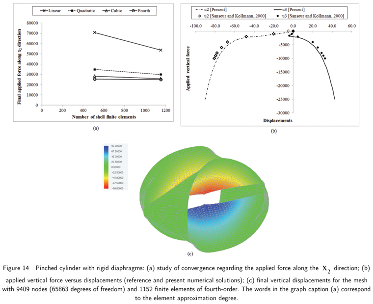
According to [27], this benchmark problem is similar to a finger-pinched beer can (see figure 13). Usually, the constitutive law employed to simulate this numerical example is the linear Saint Venant-Kirchhoff hyperelastic model (see [26,27,31,37,39], among many others). Here the adopted hyperelastic model is the nonlinear neo-Hookean law (18). The material coefficients have been found via the following transformations:

where Ε and ν are the Young modulus and the Poisson's ratio, respectively. To analyze this pinched cylinder with the Saint Venant-Kirchhoff model, the usual material coefficients are Ε = 30000.0 and ν = 0.30. Due to the symmetry regarding the planes x₁ = 100.0, x₂ = 0.0 and x₃ = 0.0, only one eighth of the cylinder is discretized. As the resultant displacement field is complex and there may be structural instabilities, two large numbers of finite elements have been adopted: 512 (16 x 16 x 2) and 1152 (24 x 24 x 2). Again, locking regarding the vertical reaction force can be avoided with mesh refinement (see figure 14a). Small differences between the present and the reference numerical solutions were expected as the adopted constitutive models are different, and these differences increase with an increasing applied force (see figure 14b). The reference solution has been obtained with 1600 (40 x 40) 4-node hybrid stress and enhanced strain shell finite elements [31]. For the most refined mesh, the final deformed configuration of the cylinder is depicted in figure 14c.

6.8 Shell finite element with six nodal parameters

In order to show the influence of the seventh parameter "a" (see equation 6) on the finite element solution, the problems of sections 6.2, 6.3, 6.4, 6.5, 6.6 and 6.7 have been numerically analyzed restricting this nodal parameter. The resultant shell finite element accounts for translations, rotations and constant strain along the thickness direction. The meshes employed here are the most refined ones for each case (see table 2). The influence of the nodal parameter "a" on the numerical results can be seen in figures 15-17, from which one can draw the following conclusions: in general, the restriction of the seventh parameter "a" of all the nodes increases the structural rigidity and, hence, leads to locking; for the Cook's membrane and the thin plate ring problems, the results are practically the same; and the difference in the deformation distribution along the thickness direction is more significant for the spherical shell in comparison with the cantilever. As expected, the restriction of the seventh parameter "a" leads to a constant stretch across the thickness (see figures 16 and 17). The similarity in figure 15b may be related to the fact that the Cook's membrane is a plane problem (despite the singularity). In figure 15d, one can note that the inclusion of the seventh parameter, which leads to a linearly variable strain along the thickness, does not influence the numerical solution, as the aspect ratio (length/thickness) of the shell is very small. The final distribution of the seventh parameter "a", for some examples, is depicted in figure 18, in which one can see that, although the restriction of this parameter has a clear influence on the structural behavior (see figures 15-17), the final value of "a" is very small when compared to the unit (except for the region around the applied force on the pinched cylinder).

Another comparison has been performed in order to show the influence of the seventh parameter "a" and the Poisson's ratio on the behavior of the pinched cylinder of figure 13. It is well known that values of Poisson's ratio close to 0.50 leads to locking problems. So, besides the first value ν = 0.30, two more values have been selected: ν = 0.45 and ν = 0,49. As the hyperelastic model is the neo-Hookean law (18), the transformations (36) and (37) are used here. The pinched cylinder has been simulated twice with these three values: the first simulation with the seventh parameter "a" free; and the second with the parameter "a" restricted. Therefore, six cases are compared to each other. According to figure 19, when the seventh nodal parameter is free, raising the value of the Poisson's ratio an acceptable structural rigidity increase is achieved, but when the parameter "a" is restricted, increasing Poisson's ratio leads to locking. Thus, using the seventh nodal parameter "a" (that is, the modeling of the linear strain across the thickness) avoids Poisson locking for homogeneous shell applications.

The results of the present section reinforce the importance of modeling the linear variation of strain along the thickness direction for shells with large displacements whose material behavior is described by nonlinear hyperelastic laws.

7 CONCLUSIONS

In this paper, a shell finite element formulation is successfully employed to the analysis of homogeneous rubber-like materials under finite deformation, statically applied forces and isothermal conditions. The kinematics of the shell is based on the Reissner-Mindlin hypothesis, and accounts for thickness change and linearly variable strain across the thickness. Shell finite elements with seven nodal parameters of any-order are employed. The generalized approximation order of the shell is implemented via a numerical strategy. Nonlinear and isotropic hyperelastic constitutive models, usually employed for near-incompressible rubber-like materials, are adopted. Some large deformation structural problems are used to validate the presented numerical formulation. In order to improve accuracy and reliability of the results, mesh refinement and full integration are performed. In the context of the shell analysis, the present paper stresses the importance of adopting high-order approximations and using the seventh parameter, which represents the linear variation of strain through the thickness direction. For moderate thick shells in bending-dominated situations, the restriction of the seventh nodal parameter leads to locking and to considerable differences in the deformation fields. In addition, the use of the seventh nodal parameter avoids Poisson locking, which is usually present when the Poisson's ratio is close to 0.50 and when the strain along the thickness direction is uniform.

Received 25 Sep 2012

In revised form 25 Jan 2013

The expressions for determination of the matrices M_coef, M_d1 and M_d2, and v_ξ the vectors v_ξ1, and v_ξ2 (see equations 31-33) are provided here.

For a two-dimensional triangular finite element of polynomial order p, the number of nodes per element is:

The internal numbering of the nodes - or the numbering of the nodes inside each element domain - is depicted in figure A1. The general expressions employed here to determine the non-dimensional coordinates ξ₁ and ξ₂ of the nodes for any element order are provided in table A1. One can note that, regarding the non-dimensional auxiliary space, the nodes with the same coordinate ξ₁ and ξ₂ are equally spaced.

For any isoparametric triangular finite element of order p, all the shape functions can be written via the following general polynomial expression:

where is the n-th coefficient of the shape function associated with node k. Expression (A2) can be rewritten in an alternative way:

This expression is the expanded form of equation (31). In order to determine the matrix of coefficients M_coef, one uses the property of the Lagrange polynomials:

where Φ_i (ξ_k) and [v_ξ(ξ_k)]_j and are the values of the shape function Φ_i and the vector component (v_ξ)_j at node k; and δ_ik is the Kronecker delta. Expanding equation (A4):

where ξ₁(k) and ξ₂(k) are the non-dimensional coordinates of node k; I is the identity matrix. As one can see, the matrix that contains the coefficients of all the shape functions is easily found via a simple matrix inversion. The determination of the matrix M_ξ and the vector v_ξ, for any element order p, is provided in tables A2 and ^A3, respectively.

The derivatives of the shape functions in respect to the non-dimensional coordinates ξ₁ and ξ₂, used to calculate the gradients (15) and (16), can be found from the general expression (A2):

Following a similar procedure of the expanded expression (A3), one can write:

These equations are the expanded forms of expressions (32) and (33), respectively. Regarding the triangular element of figure A1, the determination of the matrices M_d1 and M_d2, and the vectors v_ξ1 and v_ξ2 - for any approximation order p - are provided in tables A4 and ^A5, respectively.

• [1] H. Hakula, Y. Leino and J. Pitkäranta. Scale resolution, locking, and high-order finite element modelling of shells. Comput. Methods Appl. Mech. Engrg., 133: 157-182, 1996.
• [2] M. Suri. Analytical and computational assessment of locking in the hp finite element method. Comput. Melhods Appl. Mech. Engrg., 133: 347-371, 1996.
• [3] A. Düster, S. Hartmann and E. Rank. p-FEM applied to finite isotropic hyperelastic bodies. Comput. Methods Appl. Mech. Engrg., 192: 5147-5166, 2003.
• [4] J.N. Reddy. Mechanics of laminates composite plates and shells: theory and analysis Boca Raton : CRC Press, 2004.
• [5] R.A. Arciniega and J.N. Reddy. Large deformation analysis of functionally graded shells. International Journal of Solids and Structures, 44: 2036-2052, 2007.
• [6] Y. Basar, U. Hanskötter and Ch. Schwab. A general high-order finite element formulation for shells at large strains and finite rotations. Int. J. Numer. Meth. Engng., 57: 2147-2175, 2003.
• [7] C.S. Jog. Higher-order shell elements based on a Cosserat model, and their use in the topology design of structures. Comput. Methods Appl. Mech. Engrg., 193: 2191-2220, 2004.
• [8] E. Rank, A. Düster, V. Nübel, K. Preusch and O.T. Bruhns. High order finite elements for shells. Comput. Methods Appl. Mech. Engrg., 194: 2494-2512, 2005.
• [9] H.B. Coda and R.R. Paccola. A positional FEM Formulation for geometrical non-linear analysis of shells. Latin American Journal of Solids and Structures, 5: 205-223, 2008.
• [10] G.M. Kulikov and E. Carrera. Finite deformation higher-order shell models and rigid-body motions. International Journal of Solids and Structures, 45: 3153-3172, 2008.
• [11] J.C. Simo, M.S. Rifai and D.D. Fox. On a stress resultant geometrically exact shell model. Part IV: variable thickness shells with through-the-thickness stretching. Comput. Methods Appl. Mech. Engrg., 81: 91-126, 1990.
• [12] Y. Basar and Y. Ding. Finite-element analysis of hyperelastic thin shells with large strains. Computational Mechanics, 18: 200-214, 1996.
• [13] M. Bischoff and E. Ramm. On the physical signi®cance of higher order kinematic and static variables in a three-dimensional shell formulation. International Journal of Solids and Structures, 37: 6933-6960, 2000.
• [14] N. Büchter and E. Ramm.3d-extension of nonlinear shell equations based on the enhanced assumed strain concept. In: Hirsch, C. (Ed.), Computational Methods in Applied Sciences Elsevier, Amsterdam, pp. 55-62.
• [15] J. Bonnet, H. Marriott and O. Hassan. An averaged nodal deformation gradient linear tetrahedral element for large strain explicit dynamic applications. Commun. Numer. Meth. Engng., 17: 551-561, 2001.
• [16] H.B. Coda and M. Greco. A simple FEM formulation for large deflection 2D frame analysis based on position description. Comput. Methods Appl. Mech. Engrg., 193: 3541-3557, 2004.
• [17] R.W. Ogden. Non-linear Elastic Deformations Ellis Horwood Ltd., Chichester, England, 1984.
• [18] M.A. Crisfield. Non-linear Finite Element Analysis of Solids and Structures John Wiley & Sons, Chichester, England, 2000.
• [19] G.A. Holzapfel. Nonlinear Solid Mechanics -A Continuum Approach for Engineering John Wiley & Sons Ltd., Chichester, England, 2004.
• [20] O.H. Yeoh, Hyperelastic Material Models for Finite Element Analysis of Rubber. J. Nat. Rubb. Res., 12: 142-153, 1997.
• [21] S. Hartmann and P. Neff. Polyconvexity of generalized polynomial-type hyperelastic strain energy functions for near-incompressibility. International Journal of Solids and Structures, 40: 2767-2791, 2003.
• [22] K.Y. Sze, S.J. Zheng and S.H. Lo. A stabilized eighteen-node solid element for hyperelastic analysis of shells. Finite Elements in Analysis and Design, 40: 319-340, 2004.
• [23] J.P. Pascon. Modelos constitutivos para materiais hiperelásticos: estudo e implementação computacional Master's dissertation. São Carlos: Departamento de Engenharia de Estruturas, EESC, USP, 2008.
• [24] J. Korelc, U Solinc and P. Wriggers. An improved EAS brick element for finite deformation. Comput. Mech., 46: 641-659, 2010.
• [25] Y. Basar and Y. Ding. Shear deformation models for large-strain shell analysis. Int. J. Solids Structures, 34: 1687-1708, 1997
• [26] E.M.B. Campello, P.M. Pimenta and P. Wriggers. A triangular finite shell element based on a fully nonlinear shell formulation. Computational Mechanics, 31: 505-518, 2003.
• [27] P.M. Pimenta, E.M.B. Campello and P. Wriggers. A fully nonlinear multi-parameter shell model with thickness variation and a triangular shell finite element. Computational Mechanics, 34: 181-193, 2004.
• [28] N. Büchter, E. Ramm and D. Roehl. Three-dimensional extension of non-linear shell formulation based on the enhanced assumed strain concept. International Journal for Numerical Methods in Engineering, 37: 2551-2568, 1994.
• [29] H. Parisch. A continuum-based shell theory for non-linear applications. International Journal for Numerical Methods in Engineering, 38: 1855-1883, 1995.
• [30] N. El-Abbasi and S.A. Meguid. A new shell element accounting for through-thickness deformation. Comput. Methods Appl. Mech. Engrg., 189: 841-862, 2000.
• [31] C. Sansour and F.G. Kollmann. Families of 4-node and 9-node finite elements for a finite deformation shell theory. An assesment of hybrid stress, hybrid strain and enhanced strain elements. Computational Mechanics, 24: 435-447, 2000.
• [32] G.R. Cowper. Gaussian quadrature formulas for triangles. International Journal for Numerical Methods in Engineering, 7: 405-408, 1973.
• [33] J. N. Lyness and D. Jespersen. Moderate degree symmetric quadrature rules for the triangle. J. Inst. Maths. Applics., 15: 19-32, 1975.
• [34] D.A. Dunavant. High degree efficient symmetrical Gaussian quadrature rules for the triangle. International Journal for Numerical Methods in Engineering, 21: 1129-1148, 1985.
• [35] I.S. Duff. MA57 -A Code for the Solution of Sparse Symmetric Definite and Indefinite Systems, 2004.
• [36] A. Petchsasithon and P. D. Gosling. locking-free hexahedral element for the geometrically non-linear analysis of arbitrary shells. Comput Mech, 35: 94-114, 2005.
• [37] H.B. Coda and R.R. Paccola. An alternative positional FEM formulation for geometrically non-linear analysis of shells: curved triangular isoparametric elements. Comput Mech, 40: 185-200, 2007.
• [38] R. H. Macneal and R.L. Harder. A proposed standard set of problems to test the finite element accuracy. Finite Elements in Analysis and Design, 1: 3-20, 1985.
• [39] K.Y. Sze, X.H. Liu and S.H. Lo. Popular benchmark problems for geometric nonlinear analysis of shells. Finite Elements in Analysis and Design, 40: 1551-1569, 2004.

Appendix

Publication Dates

• Publication in this collection
  15 May 2013
• Date of issue
  Nov 2013

History

• Received
  25 Sept 2012
• Accepted
  25 Jan 2013