Comparison of semi and fully-implicit time integration schemes applied to a damage and fatigue phase field model

Abstract

In this work, we apply semi and fully-implicit time integration schemes to the damage and fatigue phase field presented in Boldrini et al. (2016). The damage phase field is considered a continuous dynamic variable whose evolution equation is obtained by the principle of virtual power. The fatigue phase field is a continuous internal variable whose evolution equation is considered as a constitutive relation to be determined in a thermodynamically consistent way. In the semi-implicit scheme, each equation is solved separately by suited implicit method. The Newton’s method is used to linearize the equations in the fully-implicit scheme. The time integration methods are compared and the results of damage and fracture evolution under the influence of fatigue effects are presented. The computational cost associated to the semi-implicit scheme showed be lower than the fully counterpart.

Keywords
Damage; fatigue; phase field; finite element method

1 INTRODUCTION

The effects of the fatigue are of great concern when designing mechanical components, as they account for the majority of mechanical failures. Modeling and simulation of fatigue accumulation can lower development time and reduce prototype and testing costs ( Lemaitre and Desmorat, 2005 ). However, some aspects such as crack initiation are rather difficult to handle in the classic models. The correct and robust assessment of such issues is challenging, but the introduction of phase field models for the evolution of damage and fatigue can overcome the main difficulties.

Originally, the phase field model was developed by John W. Cahn and John E. Hilliard to describe the phase separation in fluids through the fourth-order Cahn-Hilliard equation ( Cahn and Hilliard, 1958 ). Later on, Sam Allen and John Cahn developed the classical Allen-Cahn equation ( Allen and Cahn, 1972 ), a second-order nonlinear partial differential equation modeling phase separation in iron alloys. Both equations are based on the Ginzburg-Landau free energy functional. Recently, researchers have given more attention to phase field models, using them in a wide range of applications such as biology and medicine fields. Some of the different uses of phase field models include the study of tumor growth ( Silva, 2009 ), vesicle-fluid interation ( Du et al., 2007 ) and fluid-structure interaction problems ( Sun et al., 2014 ).

Damage, crack propagation and fatigue have also used phase field models in recent years. The works on brittle fracture showed accurate crack propagation patterns for different benchmarks ( Miehe et al., 2010a ; Miehe et al., 2010b ; Borden et al., 2014 ), see Ambati et al. (2015a) for an enlightening review on the phase field models of brittle fracture in elastic solids. Duda et al. (2015) extends the phase field damage model to describe brittle fracture in elastoplastic materials. Effects of ductile fracture are captured by the models proposed in Ambati et al. (2015b) and Borden et al. (2016) . Impressive numerical results broadening the previous phase field models are presented. Damage and fatigue phase field models were developed by Fabrizio et al. (2006) , Amendola and Fabrizio (2014) and, Caputo and Fabrizio (2015) . In those models, an expression for fatigue is given from the beginning making generalization for more complex situations rather difficult. More recently, Boldrini et al. (2016) proposed a damage and fatigue model similar to Amendola and Fabrizio (2014) . However, in this case, fatigue is treated as an internal variable with a constitutive law found in a thermodynamically consistent way. Disregarding the fatigue variable in Boldrini et al. (2016) , a model which is closely related to, but more general than Miehe et al. (2010a) , is obtained.

Boldrini et al. (2016) present a thermodynamically consistent model for non-isothermal evolution of damage and fatigue. The difference between the damage phase field $\phi$ and the fatigue internal variables $\mathcal{F}$ is in their scales: the first variable is related to meso/macro-cracks and the second one associated to micro-cracks. The results are for 1D examples, solved using high-order finite elements ( Bittencourt, 2014 ), and the explicit Runge-Kutta time integration scheme. The results had expected convergence rates for the $p$ -refinement by using manufactured solution. The simulations also showed that fatigue effects play a major role to drive the crack initiation under cyclic loading with small stresses (we remark, however, that fatigue may also evolve even under monotonic loading as discussed in Section 5.1). Temperature rises were also observed in simulations of the non-isothermal equations, in agreement with experimental observations.

Although the 1D results showed expected behavior and the explicit Runge-Kutta time integration method performed well, the solution of 2D and 3D problems is more complex due to the high computational costs. The use of an explicit time integration scheme requires smaller time increments to achieve stability, compared to the implicit methods. In this way, high dimensional problems demand finer meshes and smallest time increments for better approximations, making the use of explicit time integration methods in most cases unfeasible. On the other hand, a fully-implicit method is generally costly due to the problem and the involved non-linearities.

In the present work, we propose a semi-implicit scheme to solve the isothermal model for the evolution of damage and fatigue and which provides the desired stability, even for large time steps. In this scheme, each equation is treated separately by the suited implicit method, keeping the others variables frozen. More specifically, for each time step the evolution of one variable is solved and the results are used as input for equations of the other variables. In order to show the efficiency and accuracy of this scheme, the results are compared with the fully-implicit method obtained using the Newton’s procedure.

Section 2 presents the phase field model and the governing equations for the isothermal case and linear elastic brittle material. Section 3 shows the finite element spatial discretization for the proposed model. Section 4 describes the semi and fully-implicit schemes. For the semi-implicit case, different time integration methods are presented. Among the methods covered are Newmark, backward Euler, trapezoidal method and an implicit 2nd-order Runge-Kutta scheme called TR-BDF2. In the fully-implicit scheme, the residue and the Jacobian matrix of the Newton’s procedure are described based on the Newmark and trapezoidal methods. Section 5 describe the results for an I-shaped specimen under monotonic and cyclic loadings. From these numerical results, a convergence rate analysis is considered for different combinations of the proposed methods using the semi-implicit scheme. A comparison of the accuracy and computational time cost between the semi and fully-implicit closes this section. Finally, Section 6 outlines the conclusions of the numerical example and the aspects of the proposed schemes.

2 GOVERNING EQUATIONS

The work of Boldrini et al. (2016) presents a framework for structural damage and fatigue using thermodynamically consistent and non-isothermal phase field models. The coupled dynamic equations for the evolution of displacement $u$ , velocity $\dot{u}$ and damage phase field $\phi$ are obtained by applying the principle of virtual power and the entropy inequality based on the specific free energy potential. The damage phase field $\phi$ represents the volumetric fraction of damaged material with $\phi =0$ for a virgin material, $\phi =1$ for a fractured material and $0<\phi <1$ for damaged material between virgin and fully broken states. The evolution equation for the internal fatigue variable $\mathcal{F}$ is derived by finding a differential constitutive relation for $\mathcal{F}$ that satisfies the entropy inequality for all possible admissible processes.

From suitable choices of free-energy, initial and boundary conditions, and disregarding the temperature evolution, the isotropic isothermal case described in Eq. (62) of Boldrini et al. (2016) is

$$\{\begin{array}{l}\begin{array}{c}\ddot{u}=\text{div}\left({(1-\phi )}^2\frac{C}{{\rho }_0}E\right)+\frac{b}{{\rho }_0}\text{div(}D)-\frac{\gamma g_c}{{\rho }_0}\text{div(}\nabla \phi \otimes \nabla \phi )+f\\ \dot{\phi }=\frac{\gamma g_c}{\lambda }\Delta \phi +\frac{1}{\lambda }(1-\phi )E^{T}CE-\frac{1}{\lambda \gamma }\left[g_c{\mathcal{H}}^{\text{'}}(\phi )+\mathcal{F}{\mathcal{H}}_f^{\text{'}}(\phi )\right]{{\displaystyle }}_{}\stackrel{}{{\displaystyle }}\end{array}\\ \dot{\mathcal{F}}=-\frac{\widehat{F}}{\gamma }{\mathcal{H}}_f(\phi )\end{array}$$ , (1)

where $E={\nabla }^{s}u$ , $D={\nabla }^s\dot{u}$ and $C$ are, respectively, the infinitesimal strain tensor, the rate of strain tensor and the elasticity tensor (using Voigt notation) given in terms of the Young’s modulus $E$ and Poisson’s coefficient $\nu$ . Coefficient $b$ refers to the viscous damping of the material, $g_c$ is the Griffith fracture energy, ${\rho }_0$ corresponds to the material’s density and $\gamma >0$ is a parameter related to the width of the damage phase field layers. The parameter $\lambda$ is associated to the rate of damage change and should increase proportional to the damage as described in Lemaitre and Desmorat (2005) . It is given as

$$\frac{1}{\lambda }=\frac{c}{{(1+\delta -\phi )}^{\zeta }}$$ , (2)

where the parameters $c$ and $\zeta$ are positive and dependent on the material and $\delta$ is a small positive constant used to avoid singularity. In the present work, it is assumed $\zeta =1$ for simplicity.

Additionally, suitable potentials $\mathcal{H}$ and ${\mathcal{H}}_f$ are needed. The role of these potentials is to drive the damage from zero to one as the fatigue changes from zero to $g_c$ . Different potentials change the way that damage varies by intermediate values of fatigue. A suitable choice for the potentials is such that damage changes in a monotonic and continuous way. Here we adopt

$$\mathcal{H}(\phi )=\{\begin{array}{l}0.5{\phi }^2{{\displaystyle }}_{}{{\displaystyle }}_{}{{\displaystyle }}_{}\text{for}0\le \phi \le 1\\ 0.5+\delta (\phi -1)\text{for}\phi >1\\ -\delta \phi {{\displaystyle }}_{}{{\displaystyle }}_{}{{\displaystyle }}_{}\text{for}\phi <0\end{array}\underset{}{}\text{and}\underset{}{}{\mathcal{H}}_f(\phi )=\{\begin{array}{l}-\phi {{\displaystyle }}_{}\text{for}0\le \phi \le 1\\ -1{{\displaystyle }}_{}\text{for}\phi >1\\ 0{{\displaystyle }}_{}\text{for}\phi <0\end{array}$$ . (3)

Remark 1: The complete definitions of the potentials$\mathcal{H}(\phi )$ and ${\mathcal{H}}_f(\phi )$ , that is, their expressions for all $\phi$ , are necessary so that the hypotheses of Theorem 1 presented in Boldrini et al. (2016)on page 405 can be verified. That theorem states that necessarily$0\le \phi \le 1$ for all $t>t_0$ for sufficiently regular solutions for Eq. (1), with initial condition values in$[\mathrm{0,1}]$ at time $t_0$ , homogeneous Neumann boundary condition ( $\partial \phi /\partial n=0$ ) and under some additional hypotheses on the potentials (which the previously given $\mathcal{H}(\phi )$ and ${\mathcal{H}}_f(\phi )$ fulfill).

This means that for solutions of the continuous model (1), the damage variable$\phi$assumes values only in the interval$[\mathrm{0,1}]$ , and thus only the parts of the potentials$\mathcal{H}(\phi )$and${\mathcal{H}}_f(\phi )$associated to values of$\phi$in the interval$[\mathrm{0,1}]$are in fact used during the evolution.

However, another reason for given the complete definition of the potentials is that, when numerically solvingEq. (1)there is the possibility that some computed values of the approximation of$\phi$fall slightly outside$[\mathrm{0,1}]$ . This may happen due to discretization error, especially for rather large time steps, and thus, to guarantee that the computations may proceed, the complete definitions of the potentials are required.

Finally, the parameter $\widehat{F}$ for the fatigue evolution equation is based on the micro-cracks that are formed by cyclic loadings, even small ones. The micro-crack formation depends on how large is the stress associated to the virgin material stress (see Remark 1). Choosing a linear dependence in terms of a parameter $a$ , we have

$$\widehat{F}=a(1-\phi )\Vert CE\Vert$$ . (4)

From the choice of the potential ${\mathcal{H}}_f$ in Eq. (3b) and $\widehat{F}$ as above, the evolution equation of the fatigue in Eq. (1c) assume $\dot{\mathcal{F}}\ge 0$ in any point of the material. In particular if $\phi =1$ , the fatigue $\mathcal{F}$ variable stops increasing.

There are many possibilities for the boundary conditions in Eq. (1). For Eq. (1a), there are the cases where either the displacement or the stresses are given at certain parts of the boundary. In the case of the damage variable $\phi$ , the standard boundary condition is a homogeneous Neumann condition (null flux for $\phi$ at the boundary). There is no boundary condition associated to the fatigue $\mathcal{F}$ since Eq. (1c) is locally an ordinary differential equation.

Remark 2: Eq. (4)differs slightly of the similar expression presented originally inBoldrini et al. (2016), which considers the absolute value of the power associated to the virgin material stress instead of the stress norm. This new choice of$\widehat{F}$is due to the following physical observation: the fatigue of a material subjected to alternating loads increases proportionally to the number of cycles, rather than the velocity at which the cycles were performed. In fact, there are many possibilities to choose$\widehat{F}$ . For example, instead of the stress norm, the von Mises stress or a quadratic dependence (instead a linear as inEq. (4)) may be used. These choices should be made in order to better describe the problem of interest.

Also remark that the main advantage of using a model including the fatigue variable as in Boldrini et al. (2016) is the possibility of reaching a rather general result for the possible effects of fatigue, still preserving thermodynamical consistency. In fact, in the derivation of the model presented in Boldrini et al. (2016) , from the beginning it was just assumed that fatigue had to satisfy a differential constitutive relation, but whose specific expression and how it would interact with the other physical variables had to be determined at the final steps of the entropy condition argument. This process leaded to a general expression depending on the free-energy potential and pseudo-potential of dissipation, and thus can be applied to several classes of materials. If we had restricted the form of the constitutive expression or specified how the fatigue should interacted with the other constitutive relations, the results would be also much more restricted.

Remark 3: We observe thatEq. (1)does not guarantee$\dot{\phi }\ge 0$ . Then, the presented model allows the possibility of healing of meso and macro cracks. It is possible to adapt the model in order to prevent this healing and then have irreversible damage. For this, a history of elastic energy similar toMiehe et al. (2010b)or penalty arguments can be applied. In this work, the simpler strategy proposed by the first one is adopted.

3 SPATIAL DISCRETIZATION

This section presents the finite element approximation of Eq. (1) . For this purpose, each equation is multiplied by suitable test functions ${\omega }_1$ , ${\omega }_2$ and ${\omega }_3$ , and integrated over the domain $\Omega$ of the body. By using the Gauss theorem and after the application of the boundary conditions, we obtain the following weak form for Eq. (1):

$$\{\begin{array}{l}{\displaystyle \underset{\Omega }{\int }\ddot{u}{\omega }_{1}d\Omega }=-{\displaystyle \underset{\Omega }{\int }\frac{1}{{\rho }_0}{(1-\phi )}^{2}CE:\nabla {\omega }_1}d\Omega -{\displaystyle \underset{\Omega }{\int }\frac{b}{{\rho }_0}D:\nabla {\omega }_1}d\Omega +\\ {{\displaystyle }}_{}{{\displaystyle }}_{}{{\displaystyle }}_{}{{\displaystyle }}_{}+{\displaystyle \underset{\Omega }{\int }\frac{\gamma g_c}{{\rho }_0}}(\nabla \phi \otimes \nabla \phi ):\nabla {\omega }_{1}d\Omega +{\displaystyle \underset{\Omega }{\int }f.{\omega }_{1}d\Omega +B.T.}\\ {\displaystyle \underset{\Omega }{\int }\dot{\phi }}{\omega }_{2}d\Omega =-{\displaystyle \underset{\Omega }{\int }\frac{\gamma g_c}{\lambda }}\nabla \phi .\nabla {\omega }_{2}d\Omega +{\displaystyle \underset{\Omega }{\int }\frac{1}{\lambda }}(1-\phi )E^{T}CE{\omega }_{2}d\Omega +\\ {{\displaystyle }}_{}{{\displaystyle }}_{}{{\displaystyle }}_{}{{\displaystyle }}_{}-{\displaystyle \underset{\Omega }{\int }\frac{1}{\lambda \gamma }\left[g_c{\mathcal{H}}^{\text{'}}(\phi )+\mathcal{F}{\mathcal{H}}_f^{\text{'}}(\phi )\right]}{\omega }_{2}d\Omega \\ {\displaystyle \underset{\Omega }{\int }\dot{\mathcal{F}}{\omega }_{3}d\Omega }=-{\displaystyle \underset{\Omega }{\int }\frac{\widehat{F}}{\gamma }{\mathcal{H}}_f(\phi ){\omega }_{3}d\Omega }\end{array}$$ . (5)

The boundary terms that appear in the above weak form are denoted by $B.T.$ . They depend on the boundary conditions being considered. Due the assumed homogeneous boundary condition for the damage $\phi$ , there are no extra boundary terms in Eq. (5b).

Following the similar 2D spatial discretization presented in Chiarelli et al. (2017) , we use the finite element method to approximate the above equations. For this purpose, we consider a finite element mesh such that

$$\Omega =\underset{e=1}{\overset{nelem}{A}}{\Omega }^e{{\displaystyle }}_{}and{{\displaystyle }}_{}\Gamma =\underset{e=1}{\overset{nelem}{A}}{\Gamma }^e$$ , (6)

where ${\Omega }^e$ and ${\Gamma }^e$ are the domain and the boundary of each element $e$ , $A$ represents the assembly procedure and $nelem$ is the number of elements. In this way, the approximation in each element $e$ is written as the linear combination of the $\eta$ local nodal basis functions $N_j$ as

$$u^e=N^e{\widehat{u}}^e,{{\displaystyle }}_{}{\dot{u}}^e=N^e{\widehat{\dot{u}}}^e,{{\displaystyle }}_{}{f}^e=N^e{\widehat{f}}^e,{{\displaystyle }}_{}{\phi }^e=N_{\phi }^e{\widehat{\phi }}^e{{\displaystyle }}_{}and{{\displaystyle }}_{}{\mathcal{F}}^e=N_{\mathcal{F}}^e{\widehat{\mathcal{F}}}^e$$ , (7)

where $N^e$ , $N_{\phi }^e$ , $N_{\mathcal{F}}^e$ , ${\widehat{u}}^e$ , ${\dot{\widehat{u}}}^e$ , ${\widehat{\phi }}^e$ and ${\widehat{\mathcal{F}}}^e$ are defined by

$$N^e=\left[\begin{array}{ccccccc}{N}_1& 0& N_2& 0& \mathrm{...}& N_{\eta }& 0\\ 0& N_1& 0& N_2& \mathrm{...}& 0& N_{\eta }\end{array}\right],$$ (8)

$$N_{\phi }^e=N_{\mathcal{F}}^e=\left[\begin{array}{cccc}{N}_1& N_2& \mathrm{...}& N_{\eta }\end{array}\right],$$ (9)

$${\widehat{u}}^e={\left[\begin{array}{ccccccc}{u}_{1x}^e& u_{1y}^e& u_{2x}^e& u_{2y}^e& \mathrm{...}& u_{\eta x}^e& u_{\eta y}^e\end{array}\right]}^T,$$ (10)

$${\dot{\widehat{u}}}^e={\left[\begin{array}{ccccccc}{\dot{u}}_{1x}^e& {\dot{u}}_{1y}^e& {\dot{u}}_{2x}^e& {\dot{u}}_{2y}^e& \mathrm{...}& {\dot{u}}_{\eta x}^e& {\dot{u}}_{\eta y}^e\end{array}\right]}^T,$$ (11)

$${\widehat{\phi }}^e={\left[\begin{array}{cccc}{\phi }_1^e& {\phi }_2^e& \mathrm{...}& {\phi }_{\eta }^e\end{array}\right]}^T,$$ (12)

$${\widehat{\mathcal{F}}}^e={\left[\begin{array}{cccc}{\mathcal{F}}_1^e& {\mathcal{F}}_2^e& \mathrm{...}& {\mathcal{F}}_{\eta }^e\end{array}\right]}^T.$$ (13)

The finite element interpolations for the gradients of displacement, velocity and damage for plane state are given in terms of linear combinations of the shape function global derivatives by

$$E^e=B_u^e{\widehat{u}}^e,{{\displaystyle }}_{}{D}^e=B_v^e{\dot{\widehat{u}}}^e{{\displaystyle }}_{}and{{\displaystyle }}_{}\nabla {\phi }^e=B_{\phi }^e{\widehat{\phi }}^e$$ , (14)

where the derivative matrices are defined as

$$B_u^e=\left[\begin{array}{ccccccc}{N}_{\mathrm{1,}x}& 0& N_{\mathrm{2,}x}& 0& \mathrm{...}& N_{\eta ,x}& 0\\ 0& N_{\mathrm{1,}y}& 0& N_{\mathrm{2,}y}& \mathrm{...}& 0& N_{\eta ,y}\\ N_{\mathrm{1,}y}& N_{\mathrm{1,}x}& N_{\mathrm{2,}y}& N_{\mathrm{2,}x}& \mathrm{...}& N_{\eta ,y}& N_{\eta ,x}\end{array}\right]$$ , (15)

$$B_v^e=\text{diag(}\mathrm{1,1,}\sqrt{2}/2\text{)}{B}_u^e$$ , (16)

$$B_{\phi }^e=\left[\begin{array}{cccc}{N}_{\mathrm{1,}x}& N_{\mathrm{2,}x}& \mathrm{...}& N_{\eta ,x}\\ N_{\mathrm{1,}y}& N_{\mathrm{2,}y}& \mathrm{...}& N_{\eta ,y}\end{array}\right]$$ . (17)

Replacing the above approximations in Eq. (5) , we obtain the semi-discrete form for the $e$ -th element as

$$\{\begin{array}{l}{M}^e{\widehat{\ddot{u}}}^e=K_u^e{\widehat{u}}^e+K_v^e{\widehat{\dot{u}}}^e+w_a^e+M^e{\widehat{f}}^e\\ M_{\phi }^e{\widehat{\dot{\phi }}}^e=(P_{\phi }^e+K_c^e){\widehat{\phi }}^e+w_b^e+w_c^e\\ M_{\mathcal{F}}^e{\widehat{\dot{\mathcal{F}}}}^e=w_d^e\end{array}$$ (18)

with the operators defined by

$$M^e={\displaystyle \underset{{\Omega }^e}{\int }{(N^e)}^T(N^e)d{\Omega }^e}$$ , (19)

$$M_{\phi }^e={\displaystyle \underset{{\Omega }^e}{\int }{(N_{\phi }^e)}^T(N_{\phi }^e)d{\Omega }^e}$$ , (20)

$$M_{\mathcal{F}}^e={\displaystyle \underset{{\Omega }^e}{\int }{(N_{\mathcal{F}}^e)}^T(N_{\mathcal{F}}^e)d{\Omega }^e}$$ , (21)

$$K_u^e=-{\displaystyle \underset{{\Omega }^e}{\int }\frac{1}{{\rho }_0}{(1-N_{\phi }^e{\widehat{\phi }}^e)}^2{(B_u^e)}^{T}C(B_u^e)d{\Omega }^e}$$ , (22)

$$K_v^e=-{\displaystyle \underset{{\Omega }^e}{\int }\frac{b}{{\rho }_0}{(B_v^e)}^T(B_v^e)d{\Omega }^e}$$ (23)

$$P_{\phi }^e=-{\displaystyle \underset{{\Omega }^e}{\int }\frac{\gamma g_c}{\lambda }{(B_{\phi }^e)}^T(B_{\phi }^e)d{\Omega }^e}-{\displaystyle \underset{{\Omega }^e}{\int }\frac{g_c}{\gamma \lambda }{(N_{\phi }^e)}^T(N_{\phi }^e)d{\Omega }^e}$$ , (24)

$$K_c^e=-{\displaystyle \underset{{\Omega }^e}{\int }\frac{1}{\lambda }}{(B_u^e{\widehat{u}}^e)}^{T}C(B_u^e{\widehat{u}}^e){(N_{\phi }^e)}^T(N_{\phi }^e)d{\Omega }^e$$ , (25)

$$w_a^e={\displaystyle \underset{{\Omega }^e}{\int }\frac{\gamma g_c}{{\rho }_0}(B_{\phi }^e{\widehat{\phi }}^e\otimes B_{\phi }^e{\widehat{\phi }}^e):B_u^{e}d{\Omega }^e}$$ , (26)

$$w_b^e={\displaystyle \underset{{\Omega }^e}{\int }\frac{1}{\lambda }{(B_u^e{\widehat{u}}^e)}^{T}C(B_u^e{\widehat{u}}^e){(N_{\phi }^e)}^{T}d{\Omega }^e}$$ , (27)

$$w_c^e={\displaystyle \underset{{\Omega }^e}{\int }\frac{1}{\lambda \gamma }(N_{\mathcal{F}}^e{\widehat{\mathcal{F}}}^e){(N_{\phi }^e)}^{T}d{\Omega }^e}$$ , (28)

$$w_d^e={\displaystyle \underset{{\Omega }^e}{\int }\frac{a}{\gamma }(1-N_{\phi }^e{\widehat{\phi }}^e)(N_{\phi }^e{\widehat{\phi }}^e)\Vert C{B}_u^e{\widehat{u}}^e\Vert {(N_{\mathcal{F}}^e)}^{T}d{\Omega }^e}$$ . (29)

Note that the integrand in Eq. (26) results in a second-order tensor which is expressed as a vector using Voigt notation. Also, the potentials $\mathcal{H}(\phi )$ , ${\mathcal{H}}_f(\phi )$ and ${\mathcal{H}}_f^{\text{'}}(\phi )$ that appear in the damage and fatigue equations are given in Eq. (3) for $0\le \phi \le 1$ . The global form of the above matrices and vectors are obtained by applying the standard assembly procedure $A$ and indicated without the superscript $e$ . Appropriate choice of the elasticity tensor $C$ define particularization for plane stress or strain problems. Both could be considered; however, just the last one is used in this work.

4 TIME INTEGRATION SCHEMES

This section presents different time integration methods used by the semi and the fully-implicit procedures to solve Eq. (18) . In the semi-implicit scheme, each equation is solved separately by an implicit method. Firstly, the damage evolution equation is solved using one of three methods presented below, namely the backward Euler, trapezoidal and the 2-stage second-order accurate diagonally implicit Runge-Kutta method (TR-BDF2). The damage solution is replaced in the equation of motion which is solved by the standard Newmark method. Finally, the current displacement, velocity and damage fields are used to evaluate the fatigue by the backward Euler or trapezoidal methods. This procedure is repeated for each time step. The fully-implicit procedure is based on the iterative technique of the Newton’s method, by applying the Newmark for Eqs. (18a) and trapezoidal method for Eqs. (18b) and (18c).

Consider the split of the solution time interval $[\mathrm{0,}T]$ in discrete time steps $t_n$ with time increments given by $\Delta t=t_{n+1}-t_n>0$ for $n=\mathrm{0,1,...}$ . The global approximations for the variables are denoted at time step $t_{n+1}$ as

$$u_{n+1}=\widehat{u}(t_{n+1}),{{\displaystyle }}_{}{\dot{u}}_{n+1}=\widehat{\dot{u}}(t_{n+1}),{{\displaystyle }}_{}{\phi }_{n+1}=\widehat{\phi }(t_{n+1}){{\displaystyle }}_{}\text{and}{{\displaystyle }}_{}{\mathcal{F}}_{n+1}=\widehat{\mathcal{F}}(t_{n+1})$$ . (30)

The integration procedures used in Eq. (18) are presented in the following sections. The semi and fully-implicit algorithms are summarized at the end of their respective Sections.

4.1 Semi-implicit Scheme

This section presents the time integration procedures for Eq. (18) used in the semi-implicit scheme.

4.1.1 Damage Evolution Equation

The simplest method for time integration of Eq. (18b) in global form is the forward Euler, whose explicit scheme of evolution is given by

$${\phi }_{n+1}=\left[I+\Delta t{(M_{\phi })}^{-1}(P_{\phi ,n}+K_{c,n})\right]{\phi }_n+\Delta t{(M_{\phi })}^{-1}(w_{b,n}+w_{c,n})$$ , (31)

where $I$ is an appropriate identity matrix. In a very similar way, now considering the right-hand side in the current time step, we have the implicit backward Euler. In this case, the time-marching rule is given by the following system to be solved at each time step

$$\left[M_{\phi }-\Delta t(P_{\phi ,n+1}+K_{c,n+1})\right]{\phi }_{n+1}=M_{\phi }{\phi }_n+\Delta t(w_{b,n+1}+w_{c,n+1})$$ . (32)

Performing an average between the above two Euler methods, we obtain the implicit trapezoidal method. Unlike the Euler methods that are only first order accurate for linear problems, this method is second order accurate due to its symmetric approximation. Applying the trapezoidal method in Eq. (18b) results in the following time evolution rule:

$$\begin{array}{l}\left[M_{\phi }-\frac{\Delta t}{2}(P_{\phi ,n+1}+K_{c,n+1})\right]{\phi }_{n+1}=\left[M_{\phi }+\frac{\Delta t}{2}(P_{\phi ,n}+K_{c,n})\right]{\phi }_n+\\ \underset{}{}\underset{}{}\underset{}{}\underset{}{}\underset{}{}\underset{}{}\underset{}{}\underset{}{}\underset{}{}\underset{}{}\underset{}{}\underset{}{}\underset{}{}\underset{}{}\underset{}{}\underset{}{}\underset{}{}\underset{}{}\underset{}{}\underset{}{}\underset{}{}\underset{}{}-\frac{\Delta t}{2}(w_{b,n+1}+w_{b,n})-\frac{\Delta t}{2}(w_{c,n+1}+w_{c,n}).\end{array}$$ (33)

This work also proposes the use of the 2-stage second-order accurate diagonally implicit method, or simply TR-BDF2 method. As the backward Euler, the TR-BDF2 is a L-stable method, indicated for the time stiff problems ( LeVeque, 2007 ). The first stage consists of the trapezoidal method applied over $\Delta t$ /2 obtaining the solution ${\phi }_{*}$ . In the second stage, the solution is updated by solving the following system:

$$\left[M_{\phi }-\frac{\Delta t}{3}(P_{\phi ,n+1}+K_{c,n+1})\right]{\phi }_{n+1}=M_{\phi }\left[\frac{4}{3}{\phi }_{*}-\frac{1}{3}{\phi }_n\right]+\frac{\Delta t}{3}(w_{b,n+1}+w_{c,n+1})$$ . (34)

Unlike the others, this method requires the solution of two linear systems at each time step.

The above operators depend on the current variables, an exception is the forward Euler. However, we use the values at the previous time steps in the semi-implicit scheme. For example, in Eq. (32) is used ${\phi }_n$ , $u_n$ and ${\mathcal{F}}_n$ instead of ${\phi }_{n+1}$ , $u_{n+1}$ and ${\mathcal{F}}_{n+1}$ , respectively. This makes possible to perform the assembly of the operators, and thus the time integration. In this way, the backward Euler method applied to the damage equation becomes

$$\left[M_{\phi }-\Delta t(P_{\phi ,n}+K_{c,n})\right]{\phi }_{n+1}=M_{\phi }{\phi }_n+\Delta t(w_{b,n}+w_{c,n})$$ . (35)

The same idea is used for all the above methods.

4.1.2 Equation of Motion

Consider the system of ordinary differential equations Eq. (18a) given in the global form by

$$M\widehat{\ddot{u}}=K_u\widehat{u}+K_v\widehat{\dot{u}}+w_a+M\widehat{f}$$ . (36)

In order to approximate the solution for the displacement $u_{n+1}$ , the implicit standard Newmark procedure is adopted ( Newmark, 1952 ). In this method, the acceleration and velocity are evaluated using the updated values of the displacement by

$${\ddot{u}}_{n+1}={\alpha }_1(u_{n+1}-u_n)-{\alpha }_2{\dot{u}}_n-{\alpha }_3{\ddot{u}}_n$$ , (37)

$${\dot{u}}_{n+1}={\alpha }_4(u_{n+1}-u_n)+{\alpha }_5{\dot{u}}_n+{\alpha }_6{\ddot{u}}_n$$ , (38)

where the coefficients ${\alpha }_j$ $(j=\mathrm{1,}\dots \mathrm{,6})$ are given in terms of the Newmark coefficients $\tilde{\gamma }$ and $\tilde{\beta }$ (we assume the values $\tilde{\gamma }=0.5$ and $\tilde{\beta }=0.25$ ) by

$${\alpha }_1=\frac{1}{\tilde{\beta }\Delta t^2},\underset{}{}{\alpha }_2=\frac{1}{\tilde{\beta }\Delta t},\underset{}{}{\alpha }_3=\frac{1-2\tilde{\beta }}{2\tilde{\beta }},\underset{}{}{\alpha }_4=\frac{\tilde{\gamma }}{\tilde{\beta }\Delta t},\underset{}{}{\alpha }_5=1-\frac{\tilde{\gamma }}{\tilde{\beta }},\underset{}{}\text{and}\underset{}{}{\alpha }_6=\left[1-\frac{\tilde{\gamma }}{2\tilde{\beta }}\right]\Delta t$$ . (39)

Substituting the above approximations in Eq. (36) , we obtain the following time-marching system:

$$\left[{\alpha }_{1}M-K_u-{\alpha }_4{K}_v\right]u_{n+1}=M\left[{\alpha }_3{\ddot{u}}_n+{\alpha }_2{\dot{u}}_n+{\alpha }_1{u}_n\right]+K_v\left[{\alpha }_6{\ddot{u}}_n+{\alpha }_5{\dot{u}}_n-{\alpha }_4{u}_n\right]+w_a+M{f}_{n+1}$$ . (40)

After computing the displacement, the acceleration and velocity fields are updated using Eqs. (37) and (38) . The imposition of prescribed displacement $\overline{u}(t_{n+1})$ produces the $B.T.$ terms in Eq. (5a). This results in an additional step of update, where we should impose the velocity and acceleration at the prescribed boundary as

$${\overline{\dot{u}}}_{n+1}=\frac{d}{dt}\overline{u}(t_{n+1}){{\displaystyle }}_{}and{{\displaystyle }}_{}{\overline{\ddot{u}}}_{n+1}=\frac{d^2}{d{t}^2}\overline{u}(t_{n+1})$$ , (41)

where the bar symbol represents the prescribed degrees of freedom.

4.1.3 Fatigue Equation

For the fatigue equation Eq. (18c), we use the backward Euler and trapezoidal methods whose time evolution expressions are given respectively by

$$M_{\mathcal{F}}{\mathcal{F}}_{n+1}=M_{\mathcal{F}}{\mathcal{F}}_n+\Delta t{w}_{d,n+1}$$ , (42)

and

$$M_{\mathcal{F}}{\mathcal{F}}_{n+1}=M_{\mathcal{F}}{\mathcal{F}}_n+\frac{\Delta t}{2}\left(w_{d,n+1}+w_{d,n}\right)$$ . (43)

Note that both methods have basically the same computational cost, since $w_{d,n}$ can be treated as a stored vector.

The complete algorithm for the solution of the system is summarized in Algorithm 1 .

Algorithm 1
Algorithm of the semi-implicit time integration scheme.

Semi-implicit time integration scheme
1: for$t$from$0$to$t_f$do
2: Given $u_n$ , ${\dot{u}}_n$ and ${\lambda }_n$ use one of the Eqs. (32 – 34) to obtain ${\phi }_{n+1}$ ;
3: Given the updated damage ${\phi }_{n+1}$ , solve Eq. (40) to obtain $u_{n+1}$ ;
4: From the current displacement $u_{n+1}$ , update the acceleration ${\ddot{u}}_{n+1}$ and velocity ${\dot{u}}_{n+1}$ using
Eqs. (37) and (38), respectively; 5: Update the prescribed velocity and acceleration using Eq. (41);
6: Given $u_{n+1}$ and ${\phi }_{n+1}$ , update the fatigue ${\mathcal{F}}_{n+1}$ using Eq. (42) or (43);
7: Update the time step.
8: end

4.2 Fully-implicit Scheme

This section presents the fully-implicit scheme to solve Eq. (18) obtained from the Newton’s method. Based on the idea of linear approximation, such method is generally employed to solve nonlinear equations by an iterative sequence of linear systems ( LeVeque, 2007 ).

Consider a general nonlinear system given by

$$r(v)=0$$ . (44)

This system is solved employing some iterative procedure instead of a direct method. Supposing that $v^{(i)}$ is the approximation to $v$ at iteration $i$ , Newton’s method estimates the solution at iteration $i$ via the Taylor series expansion

$$r(v^{(i+1)})=r(v^{(i)})+\frac{\partial r(v^{(i)})}{\partial v^{(i)}}(v^{(i+1)}-v^{(i)})+\mathrm{...}$$ . (45)

Dropping the higher order terms and setting $r(v^{(i+1)})=0$ results in

$$r(v^{(i)})+\frac{\partial r(v^{(i)})}{\partial v^{(i)}}(v^{(i+1)}-v^{(i)})=0$$ , (46)

giving the following update step

$$v^{(i+1)}=v^{(i)}+\delta v^{(i)}$$ , (47)

where $\delta v^{(i)}$ solves the linear system

$$J(v^{(i)})\delta v^{(i)}=-r(v^{(i)})$$ . (48)

The Jacobian matrix $J$ and its coefficients are respectively defined as

$$J(v)=\frac{\partial r(v^{(i)})}{\partial v^{(i)}}{{\displaystyle }}_{}\text{and}{{\displaystyle }}_{}{J}_{pq}(v^{(i)})=\frac{\partial r_p(v^{(i)})}{\partial v_q^{(i)}}$$ . (49)

Newton’s method is summarized in Algorithm 2 .

Algorithm 2
Algorithm of the Newton’s method.

Fully-implicit time integration scheme
1: Specify an initial guess $v^{(0)}=v_0$ and a prescribed tolerance tol; 2: while tol < error do
3: Evaluate the Jacobian $J(v^{(i)})$ and the residue $r(v^{(i)})$ ;
4: Solve the system $J(v^{(i)})\delta v^{(i)}=-r(v^{(i)})$ for $\delta v^{(i)}$ ;
5: Update the variable $v^{(i+1)}\leftarrow v^{(i)}+\delta v^{(i)}$ ; 6: Update the iteration $i\leftarrow i+1$ ; 7: Evaluate the error as $error=\max \left[\Vert r(v^{(i)})\Vert ,\Vert \delta v^{(i)}\Vert /\Vert v^{(i+1)}\Vert \right]$ ; 8: end
9: $v\leftarrow v^{(i+1)}$

In order to solve Eq. (18) using the Newton’s method, the nonlinear system (residue) is defined by applying the Newmark in Eq. (18a) and trapezoidal method in Eqs. (18b) and (18c). This choice of time integration methods is due their high orders of accuracy presented. From Eqs. (33) , (40) , (43) and (44) the discretized nonlinear system is

$$r(u_{n+1},{\phi }_{n+1},{\mathcal{F}}_{n+1}):={\left[\begin{array}{ccc}{r}_1& r_2& r_3\end{array}\right]}^T=0$$ , (50)

whose components are

$$\begin{array}{l}{r}_1:=[{\alpha }_{1}M-K_{u,n+1}-{\alpha }_4{K}_{v,n+1}]u_{n+1}-M[{\alpha }_3{\ddot{u}}_n+{\alpha }_2{\dot{u}}_n+{\alpha }_1{u}_n]+\\ \underset{}{}\underset{}{}\underset{}{}\underset{}{}-K_{v,n+1}[{\alpha }_6{\ddot{u}}_n+{\alpha }_5{\dot{u}}_n-{\alpha }_4{u}_n]-w_{a,n+1}-M{f}_{n+1},\end{array}$$ (51)

$$\begin{array}{l}{r}_2:=\left[M_{\phi }-\frac{\Delta t}{2}(P_{\phi ,n+1}+K_{c,n+1})\right]{\phi }_{n+1}-\left[M_{\phi }+\frac{\Delta t}{2}(P_{\phi ,n}+K_{c,n})\right]{\phi }_n+\\ \underset{}{}\underset{}{}-\frac{\Delta t}{2}(w_{b,n+1}+w_{b,n})-\frac{\Delta t}{2}(w_{c,n+1}+w_{c,n}),\end{array}$$ (52)

$$r_3:=M_{\mathcal{F}}({\mathcal{F}}_{n+1}-{\mathcal{F}}_n)-\frac{\Delta t}{2}(w_{d,n+1}+w_{d,n})$$ . (53)

The Jacobian matrix can be written in the following block matrix form:

$$J=\left[\begin{array}{ccc}{J}_{11}& J_{12}& J_{13}\\ J_{21}& J_{22}& J_{23}\\ J_{31}& J_{32}& J_{33}\end{array}\right]$$ , (54)

with coefficients defined by

$$J_{p1}=\frac{\partial r_p}{\partial u_{n+1}},{{\displaystyle }}_{}{J}_{p2}=\frac{\partial r_p}{\partial {\phi }_{n+1}}{{\displaystyle }}_{}\text{and}{{\displaystyle }}_{}{J}_{p3}=\frac{\partial r_p}{\partial {\mathcal{F}}_{n+1}},{{\displaystyle }}_{}p=\mathrm{1,2,3}$$ . (55)

For the $e$ -th element, the coefficients of the Jacobian matrix are

$$J_{11}^e={\alpha }_1{M}^e-K_u^e-{\alpha }_4{K}_v^e$$ , (56)

$$J_{12}^e=-2{\displaystyle \underset{{\Omega }^e}{\int }\frac{1}{{\rho }_0}}(1-N_{\phi }^e{\widehat{\phi }}^e){(B_u^e)}^{T}C{B}_u^e{\widehat{u}}^e{N}_{\phi }^{e}d{\Omega }^e-{\displaystyle \underset{{\Omega }^e}{\int }\frac{\gamma g_c}{{\rho }_0}{(B_u^e)}^T{\tilde{B}}^e}{B}_{\phi }^{e}d{\Omega }^e$$ , (57)

$$J_{13}^e=0$$ , (58)

$$J_{21}^e=-\Delta t{\displaystyle \underset{{\Omega }^e}{\int }\frac{1}{\lambda }(1-N_{\phi }^e{\widehat{\phi }}^e)}{(N^e)}^T{(B_u^e{\widehat{u}}^e)}^{T}C(B_u^e)d{\Omega }^e,$$ (59)

$$\begin{array}{l}{J}_{22}^e=M_{\phi }^e-\frac{\Delta t}{2}{P}_{\phi }^e+\frac{\Delta t}{2}{\displaystyle \underset{{\Omega }^e}{\int }\frac{\gamma g_c}{\overline{\lambda }}}{(}^{B_{\phi }^e}(B_{\phi }^e{\widehat{\phi }}^e)(N_{\phi }^e)d{\Omega }^e+\\ \underset{}{}\underset{}{}\underset{}{}\underset{}{}+\frac{\Delta t}{2}{\displaystyle \underset{{\Omega }^e}{\int }\frac{1}{\gamma \overline{\lambda }}}(g_c{N}_{\phi }^e{\widehat{\phi }}^e-N_{\mathcal{F}}^e{\widehat{\mathcal{F}}}^e){(}^{N_{\phi }^e}(N_{\phi }^e)d{\Omega }^e,\end{array}$$ (60)

$$J_{23}^e=-\frac{\Delta t}{2}{\displaystyle \underset{{\Omega }^e}{\int }\frac{1}{\gamma \lambda }{(N_{\phi }^e)}^T}(N_{\phi }^e)d{\Omega }^e$$ , (61)

$$J_{31}^e=-\frac{\Delta t}{2}{\displaystyle \underset{{\Omega }^e}{\int }\frac{a}{\gamma \Vert C{B}_u^e{\widehat{u}}^e\Vert }(1-N_{\phi }^e{\widehat{\phi }}^e)(N_{\phi }^e{\widehat{\phi }}^e){(N_{\mathcal{F}}^e)}^T{(C{B}_u^e{\widehat{u}}^e)}^{T}C{B}_u^{e}d{\Omega }^e}{{\displaystyle }}_{}({\widehat{u}}^e\ne 0)$$ , (62)

$$J_{32}^e=\frac{\Delta t}{2}{\displaystyle \underset{{\Omega }^e}{\int }\frac{a}{\gamma }(2N_{\phi }^e{\widehat{\phi }}^e-1)\Vert C{B}_u^e{\widehat{u}}^e\Vert {(N_{\mathcal{F}}^e)}^T(N_{\mathcal{F}}^e)d{\Omega }^e}$$ , (63)

$$J_{33}^e=M_{\mathcal{F}}^e$$ , (64)

where ${\tilde{B}}^e$ and 1/ $\overline{\lambda }$ in Eqs. (57) and (60) are given respectively by

$${\tilde{B}}^e=2{\displaystyle \sum _{i=1}^{\eta }\left[\begin{array}{cc}{N}_{i,x}^e{\widehat{\phi }}_i^e& 0\\ 0& N_{i,y}^e{\widehat{\phi }}_i^e\\ N_{i,y}^e{\widehat{\phi }}_i^e& N_{i,x}^e{\widehat{\phi }}_i^e\end{array}\right]}{{\displaystyle }}_{}\text{and}{{\displaystyle }}_{}\frac{1}{\overline{\lambda }}=\frac{c}{{(1+\delta -\phi )}^2}$$ . (65)

The Jacobian matrix is non-symmetric, since $J_{31}\ne J_{13}^T$ for any $\widehat{u}\ne 0$ .

5 NUMERICAL RESULTS

This section presents the numerical results obtained using the semi and fully-implicit time integration schemes. The problem consists of the I-shaped specimen with dimensions, boundary conditions and cartesian system of coordinates given in Figure 1 . A similar problem disregarding the effects of fatigue was proposed in Chiarelli et al. (2017) . We use a mesh of quadratic quadrilaterals (serendipity element of $\eta =8$ nodes) totalizing 2700 nodes. In the present simulation, the following material and phase field parameters are used: $E=$ 180GPa, $\nu =$ 0.3, $\rho =$ 7300Kg/m³, $\gamma =$ 0.5mm, $b=5\times {10}^7$ Ns/m², $c=5\times {10}^{-4}$ m/Ns, $g_c=$ 6000N/m and $a=8\times {10}^{-9}$ m². For the iterative procedure in the fully-implicit scheme, the tolerance is $tol={10}^{-8}$ .

Figure 1
I-shaped specimen geometry and boundary conditions. Attention to detail A, where there is a reduction of 2.5% in the original width.

In order to verify the evolution of damage and fatigue, two prescribed displacement cases are considered. In the first one, a displacement of -0.1mm/s is incrementally applied through the time steps on the bottom edge, denominated case A. In the second, a sinusoidal displacement (given in millimeters) of

$$\overline{u}(t)=\{\begin{array}{l}-0.167\sin (10\pi t){{\displaystyle }}_{}{{\displaystyle }}_{}{{\displaystyle }}_{}{{\displaystyle }}_{}{{\displaystyle }}_{}\text{for}{{\displaystyle }}_{}0\le t<0.05\\ -0.075\sin (20\pi t-1.6)-0.092{{\displaystyle }}_{}\text{for}{{\displaystyle }}_{}t\ge 0.05\end{array}$$ , (66)

is applied on the same edge, called case B. A convergence study of the time integration schemes is considered in the first case. For future use, the effective and softened stress are defined as

$${\sigma }_{eff}=CE$$ , (67)

$${\sigma }_{sof}={(1-\phi )}^{2}CE+bD-\gamma g_c\text{sym}(\nabla \phi \otimes \nabla \phi )$$ , (68)

where the last term in Eq. (68) is expressed as a vector using Voigt notation. The last two terms in Eq. (68) have a small contribution to the values of the softened stress. The results are presented in the following sections.

5.1 Case A

The monotonic displacement of -0.1mm/s is incrementally applied along the time range $[\mathrm{0,1.6}]s$ on the bottom edge aims to verify the growth of the crack path in the specimen without a remarkable influence of fatigue. For illustrative purposes, Figure 2 exhibits the crack path evolution for particular time steps. Figure 3 illustrates the damage, fatigue and stress evolution for the considered time interval in the central node of the specimen. Note the fast growth of the damage levels for a small increment of time close to $t=1.4s$ , characterizing a time stiff behavior. Also, observe that the damage variable increases quickly over the time without any significant fatigue values, while the effective stress rise as time progresses. In this case, failure occurs due to the high stress levels, as expected from a tensile test. If the fatigue equation is disregard, the damage response is qualitatively the same, their values, however, are slightly smaller.

Figure 2
Damage evolution in the specimen under monotonic displacement. Results along the time: (a) $t=1.450s;$ (b) $t=1.470s;$ (c) $t=1.473s;$ (d) $t=1.475s$ and (e) $t=1.477s.$ Values obtained using the fully-implicit scheme and time increment of $\Delta t={10}^{-3}$ .

Figure 3
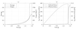
(a) Damage and fatigue. (b) Vertical stress. Results along the time at the central node of the specimen.

This problem is solved using different time integration schemes. It was verified that the use of any Runge-Kutta explicit method results in numerical instability even for small increments of time as $\Delta t={10}^{-8}$ . In order to avoid the use of small time increments, an alternative is adopting implicit time methods. Therefore, we use the Newmark procedure to solve the motion equation and the procedures previously presented in Section 4.1 for the damage and fatigue equations. In particular for the fully-implicit scheme, these last two equations are solved by using the trapezoidal method.

The use of different combinations of methods and schemes resulted in the convergence rates and CPU times given in Table 1 . The convergence rates are obtained using the relative error evaluated at $t=1.5s$ , given for a generic vector $s$ and the semi-norm by

$$\epsilon (s)=\frac{{\Vert s-s_{\text{ref}}\Vert }_2}{{\Vert s_{\text{ref}}\Vert }_2}{{\displaystyle }}_{}\text{with}{{\displaystyle }}_{}s={\displaystyle \underset{\Omega }{\int }\nabla s}\cdot \nabla sd\Omega$$ , (69)

where the reference values $s_{\text{ref}}$ are computed using the fully-implicit scheme with time increment of $\Delta t={10}^{-4}$ .

Table 1
Convergence rates for different combinations of time integration methods and the related CPU time obtained in $t=1.5s$ for time increment of $\Delta t={10}^{-3}$ .

Scheme	Equation		Convergence ratio				CPU Time
	Fatigue	Damage	Displacement	Velocity	Damage	Fatigue
Semi	BE	BE	1.62	1.30	1.64	0.78	2580
		TR	1.98	1.71	1.97	0.21	2558
		TR-BDF2	1.58	1.38	1.76	0.99	2601
	TR	BE	1.63	1.33	1.64	0.53	2585
		TR	1.92	1.45	1.15	0.28	2587
		TR-BDF2	1.58	1.40	1.36	0.97	2626
Fully	TR	TR	2.07	2.06	2.06	2.06	22512

Due to the decoupled time integration in the semi-implicit scheme, the convergence rates are below the expected theoretical values, even with the use of second-order methods. Arising from the stiff behavior, the use of the L-stable TR-BDF2 method presented the highest average rates of convergence when compared to the others methods for the damage equation. No significant difference is observed in the rates of the trapezoidal method in the fatigue equation. In general, all combinations of methods presented the same computational cost. The error values when using trapezoidal and TRBDF2 for fatigue and damage equations are illustrated in Figure 4 a. In order to obtain error below $5\%$ for the velocity, a time increment of $\Delta t={10}^{-4}$ is required. For the other variables as displacement, damage and fatigue, the increment of $\Delta t=5\times {10}^{-4}$ is sufficient.

Figure 4
Error by using: (a) Trapezoidal and TR-BDF2 in the semi-implicit. (b) Fully-implicit. Results along the time increment in log scale.

The full scheme shows quadratic rate, as expected due the use of second-order accurate methods. The error values illustrated in Figure 4 b are below $0.5\%$ for all variables. However, the computational cost is approximately $850\%$ higher than the semi-implicit scheme. In this analysis, the Jacobian matrix conditioning number had values of order $\mathcal{K}(J)={10}^{17}$ .

5.2 Case B

In this case, the sinusoidal displacement given in Eq. (66) is applied along the time range $[\mathrm{0,2.5}]s$ . The objective of this new boundary condition is to verify the growth of the crack path in the specimen with influence of the fatigue. For illustrative purposes, Figure 5 shows the damage evolution in the I-shaped specimen for particular time steps.

Figure 5
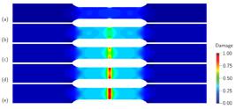
Damage evolution in the specimen under sinusoidal displacement. Results along the time: (a) $t=1s;$ (b) $t=2.3s;$ (c) $t=2.36s;$ (d) $t=2.37s$ and (e) $t=2.38s.$ Values obtained using the semi-implicit scheme and time increment of $\Delta t={10}^{-3}$ .

Conversely to the monotonic displacement, the growth of damage is largely due to fatigue. This can be seen in Figure 6 a, which illustrates the evolution of damage and fatigue along the time interval for the central node. Note that the fatigue grows at an approximately constant rate over the time, reaching large values close to failure. This results in an abruptly growth of the damage close to 2.35s, characterizing again the stiff behavior of the damage equation. In absence of fatigue, the damage grows only due the contribution of the elastic energy and their value is limited by $\approx 0.1$ . Figure 6 b shows the effective and softened stress levels evaluated at the central node of the specimen. The effective stress does not exhibit remarkable growth in magnitude over time when compared to the case A, except near failure.

Figure 6
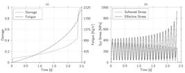
(a) Damage and fatigue. (b) Softened and effective stress levels. Results along the time at the central node of the specimen under sinusoidal prescribed displacement.

6 CONCLUSIONS

This work proposed the use of semi and fully-implicit schemes to perform the time integration of the phase field equations of damage and fatigue presented in Boldrini et al. (2016) . The explicit Runge-Kutta methods showed to be unfeasible for 2D examples, presenting instability with time increments as small as $\Delta t={10}^{-8}$ . An alternative to avoid the use of small time steps maintaining stability is to use implicit methods. The fully-implicit method presented quadratic convergence and lower errors when compared to the semi-implicit procedures. However, the fully-implicit scheme has some drawbacks:

• The Jacobian of Newton’s method is hard to obtain and becomes particular to the problem;

  • This model deals with phenomena from micro to macro-scale, then the resulting iterative system of the Newton’s method is poorly conditioned, even with the use of preconditioners;

• The Jacobian matrix is non-symmetric;

• There is a high computational cost and memory demand, since it is necessary to solve a large system in each Newton’s iteration;

The semi-implicit procedure overcomes these difficulties. In this scheme, the equations are decoupled and solved separately by suited implicit time integration procedures. Different alternatives were used for the damage equation and the TR-BDF2 method showed better accuracy with no significant additional cost. This method is L-stable and therefore suitable to solve a stiff problem as the damage equation. For the fatigue evolution equation, the trapezoidal and backward Euler methods performed similarly. For the equation of motion, only the standard Newmark procedure was used. The convergence rates for the semi-implicit scheme were below ranging close to the linear rate in most of the equations. Accurate responses (error below $5\%$ ) for displacement, damage and fatigue are possible to obtain by using time increments of $\Delta t=5\times {10}^{-4}$ . Although the velocity has high errors, this fact did not affect the displacement solution and consequently the damage and fatigue variables.

Although not applied in this work, an iteration of correction in the semi-implicit procedure would reduce errors. In particular, the prediction/correction Adams-Bashforth/Moulton methods can be used to improve accuracy. Further study on this subject will be carried out in the future.

In general, the numerical results for the I-shaped specimen for tensile and fatigue tests show the expected behavior qualitatively. The model proposed in Boldrini et al. (2016) makes possible to represent the evolution of the damage under cyclic loads due to the fatigue. This feature provides the identification of regions of initiation and propagation of cracks efficiently with a reasonable computational cost.

As the next step, we will adjust this model quantitatively with experimental tests.

7 ACKNOWLEDGEMENTS

Authors would like to thank the São Paulo Research Foundation (FAPESP) under grants 2013/50238-3, 2015/10310-2 and 2015/20188-0, the Coordination for the Improvement of Higher Education Personnel (CAPES) under grant 33003017, and also the National Council for Research and Development (CNPq) under grant 306182/2014-9.

• http://dx.doi.org/10.1590/1679-78254383

References

• Allen, S.M., Cahn, J.W., (1972). Ground state structures in ordered binary alloys with second neighbor interactions. Acta Metallurgica, 20(3):423–433.
• Ambati, M., Gerasimov, T., de Lorenzis, L., (2015a). A review on phase-field models of brittle fracture and a new fast hybrid formulation. Journal of Computational Mechanics, 55(2):383–405.
• Ambati, M., Gerasimov, T., de Lorenzis, L., (2015b). Phase-field modeling of ductile fracture. Journal of Computational Mechanics, 55(5):1017–1040. doi:10.1007/s00466-015-1151-4.
  » https://doi.org/10.1007/s00466-015-1151-4
• Amendola, G., Fabrizio, M., (2014). Thermomechanics of damage and fatigue by a phase field model. arXiv preprint arXiv:1410.7042.
• Bittencourt, M.L., (2014). Computational solid mechanics: Variational formulation and high order approximation. CRC Press.
• Boldrini, J.L., de Moraes, E.A.B., Chiarelli, L.R., Fumes, F.G., Bittencourt, M.L., (2016). A non-isothermal thermodynamically consistent phase field framework for structural damage and fatigue. Computer Methods in Applied Mechanics and Engineering, 312(395–427).
• Borden, M.J., Hughes, T.J.R., Landis, C.M., Verhoosel, C.V., (2014). A higher-order phase-field model for brittle fracture: Formulation and analysis within the isogeometric analysis framework. Computer Methods in Applied Mechanics and Engineering, 273:100–118.
• Borden, M.J., Hughes, T.J.R., Landis, C.M., Anvari, A., Lee, I.J., (2016). A phase-field formulation for fracture in ductile materials: Finite deformation, balance law derivation, plastic degradation, and stress triaxiality effects. Computer Methods in Applied Mechanics and Engineering, 312:130–166.
• Cahn, J.W., Hilliard, J.E., (1958). Free energy of a nonuniform system. I. Interfacial free energy. The Journal of chemical physics, 28(2):258–267.
• Caputo, M., Fabrizio, M., (2015). Damage and fatigue described by a fractional derivative model. Journal of Computational Physics, 293:400–408.
• Chiarelli, L.R., Fumes, F.G., de Moraes, E.A.B., Haveroth, G.A., Boldrini, J.L., Bittencourt, M.L., (2017). Comparison of high order finite element and discontinuous Galerkin methods applied to phase field equations: Application to structural damage. Computers & Mathematics with Applications, http://dx.doi.org/10.1016/j.camwa.2017.05.003.
  » http://dx.doi.org/10.1016/j.camwa.2017.05.003
• Du, Q., Li, M., Liu, C., (2007). Analysis of a phase field Navier-Stokes vesicle-fluid interaction model. Discrete and Continuous Dynamical Systems Series B, 8(3):539.
• Duda, F. P., Ciarbonetti, A. Sánchez, P. J. Huespe, A. E., (2015). A phase-field/gradient damage model for brittle fracture in elastic-plastic solids. International Journal of Plasticity, 65:269-296
• Fabrizio, M., Giorgi, C., Morro, A., (2006). A thermodynamic approach to non-isothermal phase-field evolution in continuum physics. Physica D: Nonlinear Phenomena, 214(2):144–156.
• Lemaitre, J., Desmorat, R., (2005). Engineering damage mechanics: ductile, creep, fatigue and brittle failures. Springer Science & Business Media.
• LeVeque, R.J., (2007). Finite difference methods for ordinary and partial differential equations: steady-state and time-dependent problems, Society for Industrial and Applied Mathematics.
• Miehe, C., Hofacker, M., Welschinger, F., (2010a). A phase field model for rate-independent crack propagation: Robust algorithmic implementation based on operator splits. Computer Methods in Applied Mechanics and Engineering, 199(45):2765–2778.
• Miehe, C., Welschinger, F., Hofacker, M., (2010b). Thermodynamically consistent phase-field models of fracture: Variational principles and multi-field FE implementations. International Journal for Numerical Methods in Engineering, 83(10):1273–1311.
• Newmark, N.M., (1952). Computation of dynamic structural response in the range approaching failure. Department of Civil Engineering, United States.
• Silva, S.P.L.D.d., (2009). Phase-field models for tumor growth in the avascular phase. Ms. Thesis. University of Coimbra, Portugal.
• Sun, P., Xu, J., Zhang, L., (2014). Full Eulerian finite element method of a phase field model for fluid–structure interaction problem.” Computers & Fluids, 90:1–8.

Publication Dates

• Publication in this collection
  14 June 2018
• Date of issue
  2018

History

• Received
  09 Aug 2017
• Reviewed
  07 Mar 2018
• Accepted
  23 Mar 2018