The dispersion curve applied in guided wave propagation in prismatic rods.

Abstract

The early detection of failures in structures is a subject of great interest in engineering; several of these techniques are linked with the elastic wave propagation, using guided waves is one of these alternatives. Several structures of interest in engineering are laminar arrangements; the wave propagation in this type of structures depends not only on the material properties, but also on the geometric parameters, such as the plate thickness. Tubular structures, pressure vessels, tanks and also parts of ships hulls could be considered laminar. The elastic wave propagation in laminar structures could be considered as a sum of modal shapes that have its wave length and frequencies defined. These mode families are characteristics of each structure and could be represented through the dispersion curves. The definition of these dispersion curves is of crucial importance to understand the propagation of guided waves in the structure studied. In the present work the dispersion curves were generated using three different methodologies, specific for metallic rectangular stems that compound the strengthening armor in flexible riser duct. Each approach presented in the analysis were carried out using standard finite element commercial packages and an experimental verification, as well. The premise is to present the topics in the simplest way, not only to understand how the dispersion curves are built but also how these curves must be interpreted.

Keywords
Dispersion curves; guided waves; nondestructive test; laminar structures; Finite Element Methods

1 INTRODUCTION

There are different ways to detect defects in metallic structures. They are always of great potential in engineering, especially in structures, where a failure is linked to catastrophic scenarios like pressurized structures for example. In this context, the guided waves are presented as a non-destructive technique (NDT).

In the present work different numerical approaches are shown to compute the dispersion curves which permit characterizing the wave propagation in the geometry studied, i. e., focused in rectangular metallic rods. This geometry could be employed as a component in different composite structures, for instance, in the study of the structural layer of flexible pipes (riser) used commonly in the offshore oil industry (see Fig 1.a ). The original motivation of the present work is to develop a NDT based on wave propagation that allows detecting damage in a critical region of the riser close to the platform connection (see Fig 1.b ). When a rectilinear rectangular wave guide was analyzed as an armor rise element, some important characteristics were simplified: its transversal shape, that is not perfectly rectangular, and the influence of the helicoidal shape in the longitudinal direction. Nevertheless the above mentioned characteristics could be included in the model, after this first approximation . Details about the application of the NDT based on guided waves in this kind of structures can be seen in Costa et. al. (2003) and Li et. al. (2014) .

Figure 1
(a) The different layers of the riser, (b) The region of the riser (connection at platform) that could be monitored using techniques based on guided wave propagation. Adapted from 4subsea (2018)

The original point of the work is focused in the fact that all numerical approaches presented were implemented in commercial finite element packages ( ANSYS(2009) , LS-DYNA(2003) , COMSOL(2012) ), and a special care was taken to present the theoretical topics in the simplest way, not only to understand how the dispersion curves are built, but also how these curves must be interpreted. In Åberg & Gudmundson (1997) a comparison of results obtained with standard commercial Finite Element Packages was also presented, but in that case, the focus is the computation of dispersion relations in periodic microstructures. Here an experimental test is also shown, with the aim to verify the consistency of the theoretical results obtained.

2 BIBLIOGRAPHY REVIEW

Here theoretical topics and a literature review are presented. They will be useful to understand the applications presented in the following sections.

As presented in Rose (2014) , all laminar structures, characterized by having one dimension smaller than the others, is naturally a wave guide. In a continuum media a punctual perturbation will propagate through a laminar structure according to particular patterns related to each analyzed geometry and mechanical properties. The particular patterns of each guide can be interpreted with the help of the dispersion curves.

The elastic waves that propagate in the laminar structures can be considered as a linear collection of wave modes characterized by two parameters: the wave length and its frequency. These wave modes are specific of each structure and can be represented by mean of the dispersion curves.

Each particular kind of laminar structure has its set associated with dispersion curves. It is worth mentioning that the dispersion curves are a tool to understand the wave propagation in the studied geometry. These curves are like a map that contains all the possible wave modes that can be propagated in a specific guided wave for each combination of frequency and wave number.

For this reason dispersion curves are a tool that could be used to characterize a propagation of guided waves in its application in non destructive techniques.

The success of the guided wave technique is based on the selection of the best wave mode that could be excited related with each specific application as indicated in Wilcox et. al. (2003) . Thus, the dispersion curve computation is the first step in implementing this kind of technique.

The dispersion curves are a set of curves that represent the propagation of wave modes that are found in a specific geometry. The dispersion curves could be presented in different domains: frequency vs wave number; wave length vs frequency; phase velocity vs frequency; and group velocity vs frequency. These curves allows to observe the dispersion associated with each wave mode.

The first work in which a harmonic solution was used to solve the problem linked with propagation was published by Pochhammer (1876) . In this paper the author solves the propagation problem of a cylindrical wave guide, generating the first dispersion related to mechanical stress waves. The same solution was obtained independently by Chree (1889) .

In a chronologic sequence, Lamb (1916) presented the dispersion curve concept when the harmonic solution was used in the problem studied by Rayleigh, who carried out a simplification of the Navier´s equation applied to plates. These equations are known as the Rayleigh–Lamb equations and will be presented in section 3.3.

Nowadays, there are new versions of the Rayleigh–Lamb equations that are adapted to other boundary conditions. As an example of this it is possible to refer to the work of Banerjee & Kundu (2006) where the dispersion curves are computed for corrugated plates in an analytical way using as a base the Rayleigh-Lamb equations.

A strategy that allows the dispersion curve computation with more flexibility, when non conventional geometries or boundary conditions are used, is the one called semi-analytical finite element method (SAFE). This strategy combines the spatial-time discretization using a finite element method and analytical methodologies to determine the wave modes that propagate in geometries with one or two infinite dimensions.

The earlier works that present this hybrid nature (combining numerical and analytical approaches) were published by Lagasse (1973) who developed theoretically and validated experimentally a SAFE method for wave guides. In this method, the domain of the transversal section is discretized by triangular finite element methods and in the wave propagation a harmonic series is assumed to interpolate the displacement fields. In this method, four types of boundary conditions (free, symmetry, antisymmetric and fixed) were implemented to simulate the different wave modes. Aalami (1973) proposed a SAFE method that used a finite element with triangular prisms whose height were oriented in the direction of the wave propagation. In this case, harmonic functions defined the displacement field in the guided wave direction. Using this strategy, an eigenvalue problem is reached, where the eigenvalues are associated with the mode wave frequencies and the model length, fixed a priori, is linked with the wave length. With this method it is possible to model guided waves with arbitrary transversal section, built with homogenous orthotropic material.

In the following decade Huang & Dong(1984) presented a SAFE method using the same approach proposed by Alami in (1973), but applied to anisotropic cylinder. In this version of SAFE the evanescent modes (associated to complex wavenumbers) are also computed. In the same line of work, Gavric (1994 , 1995 ) developed a similar method applied in rail profiles.

In the last years new SAFE methods were proposed to supply new engineering demands and to model more complex structures used in different fields of Engineering. As example, it is possible to mention tubes with different material covers, or multilayered tubes. These structures demand a non destructive testing in the structural health monitoring context.

Among the works developed using SAFE methods in the last decade, it is possible to cite the following works: Wilcox et. al (2002) that presents an alternative way to represent the guided wave infinite dimension considering a ring, with big radius, concerning the transversal section of the wave guide. In this model, an axial symmetry was assumed and the Finite Element commercial Package to compute the modal analysis in axisymmetric model, fixing the mode length in the circumferential direction, was improved, being the first to use a non-specialized FEM commercial Package to develop a SAFE method; Cegla (2008) used the same method in the propagation of metallic rectangular bars; Bartoli et. al. (2006) improved the proposal previously presented by Lagasse (1973) and Aalami (1973) . In this proposal a SAFE method was presented in which it discretizes only the wave guide transversal section and, in the propagation direction, the displacements are conveniently described using harmonic exponential functions. This approach generates a computational economy, because the finite element method applied is 2D and simple polynomial functions are used in the longitudinal domain. In this model, it is possible to simulate wave propagation with small length without extra computational cost. Other great contribution, in the use of the hybrid methods, is the possibility to simulate the material viscoelastic effect. This effect considers the elastic modulus as a complex number; methodologies based on SAFE for the case of multilayered tubes with viscoelastic properties are presented in Simonetti and Cawley (2003) , Castaings & Bacon (2006) and Predoi (2014) ; Zuo et. al. (2016) present a SAFE method combined with non-linear methods that obtain a set of more complete dispersion curves.

If a longitudinal wave with a convenient frequency is applied in a bar aiming to detect a defect inside (50KHz was used in the guided wave analyzed in the present paper), the kind of mode wave in which the reflected wave is decomposed indicates the type and severity of defect, due to the reflexion, giving information for the defect characterization. In Demma et. al.(2004) , Duan & Kirby (2015) and Glushkov et al. (2017) this kind of analysis, in the case of defects in pipes, is carried out. In Ramatlo et. al. (2016) these techniques to determine defect are applied in rails.

Also it is important to mention researches that combine wave propagation in non linear elasticity material where a specific strain field is applied allowing to modify the wave propagation conditions in the studied domain. This topic opens several possibilities of applications in Engineering and can be found in Shearer et al (2015) , Golgoon et al (2016) , Barnwell et. al. (2016) , Barnwell et. al. (2017) and Golgoon & Yavari (2017) , Golgoon & Yavari (2018) .

In the present work, a review of recent SAFE methods that use standard FE packages in their implementation was performed. The three methods implemented are explained in Predoi et. al.(2007) , Cegla(2008) and Sorohan et. al. (2011) . The dispersion curves for the prismatic bars are presented. Then, the simulation of wave propagation, when Tune Burst perturbation is applied, was performed. The analysis about how this perturbation is decomposed in the wave modes, characterized by the dispersion curves, is made. Finally, an experimental verification to show the consistency of the simulations is carried out.

3 THEORETICAL FOUNDATIONS

In the present section, first the fundamental characteristics of the wave propagation in the continuum are pointed out, then a plate as guide wave with only one finite dimension in the domain is considered. Initially, the simplest case where the wave propagate in a fluid closed between two boundaries (only dilatational waves appears) is studied. Then, a solid plate, considering also the distortional waves appearance, is analyzed. Finally, the wave guide with two finite dimensions is discussed.

3.1 Wave propagation in a rod

The expression that describes the displacement (in the unidirectional case), during the wave propagation is:

$u\left(x,t\right)=f\left(x-ct\right)$ , (1)

where u represents the displacement, t the time, x the position, c the wave propagation velocity and f a function that represents the initial excitation shape. The eq. 1 is verified as the dynamic equilibrium equation presented as follows:

$\frac{{\partial }^{2}u}{\partial x^2}=\frac{1}{c}\frac{{\partial }^{2}u}{\partial t^2}.$ (2)

In this way, the Exp. (1) is validated as displacement solution. This solution is known as the D’Alambert solution. In Fig. 2 it is illustrated how the function of u, presented in the Exp. (1) is modified in two different times. The Exp. (2) also shows that the function represented by Exp. (1) moves in space at c wave propagation velocity, this parameter is a material property of the solid.

Figure 2
One-dimensional wave propagation, without distortion and losses. t₀<t ₁.

The propagation wave velocity in the solid is constant and can be computed using Exp. (3) ,

$c=\Delta x/\Delta t$ , (3)

where $\Delta x$ and $\Delta t$ represent the intervals of space and time of the movement, respectively.

If we consider that the excitation will be a harmonic function, it is possible to write the Exp. (1) as follows:

$u\left(x,t\right)=Acos\left(\omega t-kx\right),$ (4)

where $\omega$ is the angular frequency and $k$ is the wave number, $T\left[\text{s}\right]$ represents the wave period and $\lambda \left[\text{m}\right]$ the wave length, in this way:

$\omega =2\pi /T\text{,}k=2\pi /\lambda$ . (5)

The link between the general solution presented in Exp. (1) and Exp. (4) is obtained using the relation $\lambda =cT$ , based on the Exp. (3) . The ratio between the frequency and the wave number is the so called phase velocity:

$c=\omega /k$ . (6)

This expression is useful because it enables to compute the harmonic wave propagation velocity.

Also the definition of group velocity as the derivative of frequency with respect to the wave number is used, that is

$$C_g=dw/dk$$ (7)

Using the Fourier series it is possible to represent every periodic function as a linear combination of harmonic functions, therefore knowing the harmonic wave propagation is fundamental in the study of the elastic wave propagation.

3.2. Propagation of the inclined excitation in a flysheet of fluid.

As a simple application of waveguide propagation, the case of a perturbation in a flysheet of fluid, was considered. In this case, only dilatational waves happen, because the fluid medium does not present shear strength. In the reflection analysis on the flysheet boundaries, total reflection were considered.

According to Royer & Dieulesaint (1996) , considering an infinite plate of fluid the perturbation that focuses obliquely on one of the boundaries propagates as indicated in Fig. 3 . The perpendicular lines on the wave vector k represents the wave front. These lines represent the particles that move together, oscillating around the equilibrium position. In the lamina of fluid it is only possible to have harmonic perturbation of extension and contraction, which are parallel to the wave number vector. In this case the reflection is symmetric in relation to the perpendicular line of the boundary in the wave incident point. The boundary reflection is more complex in solids, this topic will be treated ahead.

Figure 3
Guided waves propagation in a flysheet of fluid with thickness L, and with boundaries perfectly reflexive. Royer & Dieulesaint (1996) .

It is possible to carry out a decomposition of the wave vector k into two components across the spatial coordinates, indicated in the Fig. 3 , $x_1$ and $x_2$ . Notice that the wave number in the direction $x_2$ , k_2, must be an integer multiple of $\pi /L$ for a resonance condition to happen. In this direction the plate works as a resonator in which a stationary wave remains between the plate boundaries. For values of wave numbers k ₂ that are not integer, when multiplied by $\pi /L$ , the respective mode will be evanescent (propagation mode that tends to disappear), according to these premises it is possible to obtain the followings equations:

$k=k_1+k_2$ , (8)

${\beta }^2=k^2-k_2{}^2=k^2-{\left(\frac{n\pi }{L}\right)}^2$ , (9)

$C_f=\frac{\omega }{k}$ , (10)

$\omega =C_f{\left[{\beta }^2+{\left(\frac{n\pi }{L}\right)}^2\right]}^{\raisebox{1ex}{$1$}\!\left/ \!\raisebox{-1ex}{$2$}\right.}$ . (11)

It is possible to observe, in the formulation presented above, that each propagation mode is linked to an integer number n in which odd values of n generate asymmetric modes and pair values of n generate symmetric modes. The graphic presented in Fig. 4 shows five propagating modes associated to five integer values n. In this particular case $C_f$ and $L$ are being considered unitary. In a real situation the reference velocity $C_f$ is one of the medium wave propagation velocities and can be obtained using the material properties, as it will be showed ahead in Exps.( 17 - 18 ).

Figure 4
Dispersion curves of a fluid flysheet of unitary thickness

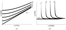
The Dispersion curve presented in Fig. 4 (a) shows a set of modal waves that depends on the angular frequency $\omega$ and the wave number $\beta$ . In Fig. 4 (b) the same information is presented in terms of the phase velocity $C_f$ , (defined in Exp. (10) ) versus the angular frequency $\omega$ .

In Fig 4 (b) notice that when the graphics lines became vertical the cut-off frequencies, are the limit frequencies for the existence of the respective modes in the analyzed structure. This characteristic of the dispersion curves is also mentioned by Rose (2014) .

In this section, the case of the flysheet fluid was considered to illustrate the shape that these curves take in this situation, without an additional complication that happens when the shear waves also interact.

Next a solid plate is considered. Its geometry simplifies the dispersion curve calculus. The plate was the first geometry completely studied in the wave propagation point of view, as cited in Auld (1973) .

3.3 The wave propagation in isotropic elastic plates.

When the wave propagates in an infinite solid plate, the interaction between the longitudinal and shear waves introduce a bigger complexity on the studied problem. This interaction is governed by the Snell law as illustrated in Fig. 4 . Lamb’s equations must be solved simultaneously and the possible solutions could be presented as a set of dispersion curves. This problem is treated in classical books of elastodynamic as in Auld (1973) and Graff (1975) .

Snell’s Law: When the wave propagates in a solid medium and reflects at its boundary, it will be separated in two waves, longitudinal and transversal . The Snell-Descartes law was developed initially for the wave light, but can be applied in other types of waves, as in the present case, the elastic waves.

This law governs the wave reflection and refraction in the interface where the propagation media changed. Considering a free boundary, the wave arrives at it and will be totally reflected.

Considering an incident pure shear wave, the incidence angle is ${\theta }_i$ . The Exp. (12) defines the exit angle ${\theta }_{rl}$ of the longitudinal wave generated by the reflection, where $c_1$ and $c_2$ are the longitudinal and transversal wave speeds in the medium.

$\frac{sin{\theta }_{rl}}{c_1}=\frac{sin{\theta }_i}{c_2}$ . (12)

Fig. 5 , illustrated the explained example

Figure 5
Free border reflection according to the Snell-Descartes law. Moore, Miller & Hill (2005) .

Notice also that the transversal reflected wave will be normal in relation to the transversal incident wave, verifying the relation, ${\theta }_{rt}+{\theta }_i={90}^o$ . There is a similar version of the Exp. (12) for the case in which the incident wave will be longitudinal.

Rayleigh-Lamb equation: Expressions 13 and 14 present the Rayleigh-Lamb equations that govern the propagation of oblique waves in a plate with thickness b, present in Auld (1973) , for a transversal incident wave. Similar expressions could be presented for the longitudinal incident wave.

$\frac{\text{tan}\left(k_{ts}b/2\right)}{\text{tan}\left(k_{tl}b/2\right)}=-\frac{{\left(k_{ts}{}^2-{\beta }^2\right)}^2}{4{\beta }^2{k}_{tl}{k}_{ts}},$ (13)

$\frac{\text{tan}\left(k_{ts}b/2\right)}{\text{tan}\left(k_{tl}b/2\right)}=-\frac{4{\beta }^2{k}_{tl}{k}_{ts}}{{\left(k_{ts}{}^2-{\beta }^2\right)}^2},$ (14)

where

$k_{tl}{}^2={\left(\frac{\omega }{c_1}\right)}^2-{\beta }^2,$ (15)

$k_{ts}{}^2={\left(\frac{\omega }{c_2}\right)}^2-{\beta }^2$ , (16)

$c_2=\sqrt{\frac{\mu }{\rho }},$ (17)

$c_1=\sqrt{\frac{\widehat{\lambda }+2\mu }{\rho }}.$ (18)

The Exps. (13) and (14) presents the relation between the wave number in the propagation direction $\beta$ and the frequency $\omega$ for the symmetric and antisymmetric modes, respectively. These expressions are written in terms of plate density $\rho$ , the Lamé constants, $\mu$ and $\widehat{\lambda }$ , and the plate thickness $b$ . Finally, $k_{ts}$ and $k_{tl}$ represents the wave numbers for the transversal and longitudinal waves in the transversal direction according to the propagate direction. $c_1$ and $c_2$ are the propagation speeds of the dilatational and equivolumial waves that were also used in the Exp. (12) .

The set of possible waves obtained from the combination of $\beta$ and $\omega$ that verifies the Rayleigh-Lamb Exps. (13) and (14) could be plotted as curve families that are presented in Fig. 6.a. In Fig. 6 (b) the same results are presented in terms of the propagation velocity (also called the phase velocity)C_f vs. the frequency $\omega$ . The Figs 6.a and b were computed for titanium plate with 10mm of thickness (Longitudinal Elastic Modulus of 120 [GPa], and Transversal Elastic Modulus of 44 [GPa]). Also the letters S and A indicate the symmetric and antisymmetric wave modes. The S wave modes are symmetric in relation to the axis $x_1$ and are antisymmetric in relation to the axis $x_2$ , the A wave modes are symmetric in relation to the axis $x_2$ and are antisymmetric in relation to the axis $x_1$ , as indicated by Rose (2014) .

Figure 6
Dispersion curves of Titanium plate with 10 mm of thickness.

Notice the similarity between the Exps.( 13 – 16 )for the solid plate and the Exps. ( 8 – 11 ) for the fluid plate. The last ones present only the longitudinal waves. Also, there is another propagation mode in plates called SH that develops into $x_3$ direction; this wave mode could be represented with dispersion curves as it is explained in Auld(1973) .

The superposition of the dispersion curves related to a plate with thickness $b_1$ and to a plate with thickness $b_2$ results in the dispersion curves associated to the rectangular bar with transversal section $b_1$ x $b_2$ . But, as observed by Cegla(2008) , the set of curves obtained in this way is not complete.

3.4 Dispersion curves of isotropic and elastic structures with finite dimension

In the case of laminar elastic structures as a duct or rail profile, the dispersion curves determination are more complex because there are not theoretical solutions, for this reason the alternative is to use numerical techniques. The finite element method combined with special boundary conditions or with analytical solution are widely used ways to reach this aim. Methods based on the combination between numerical techniques and analytical solutions are called Hybrid Methods and in the specialized literature are called by the initials SAFE(Semi Analytical Finite Element Method), Rose (2014) .

3.5 Wave propagation in isotropic elastic beam with infinite length.

Working in low frequencies there are fundamental wave modes of propagation in beams (two of bending, one longitudinal and one torsional). The wave propagation velocity c _L presented in the Exp. (19) , solves the equilibrium equation of a beam model. Its deduction is presented in Graff(1975) . This is one of the few theoretical solutions in elastodynamic. It is also possible to obtain the analytical solution of the wave propagation for the torsion wave mode. The speed of the this wave propagation is presented in Exp. (19) called c_T.

$c_L=\sqrt{\frac{E}{\rho }},c_T=\sqrt{\frac{GJ}{\rho I_0}},$ (19)

where $E$ is the elastic modulus,, $G{I}_0$ represents the torsion stiffness, $I_0$ represents the polar moment inertia and $\rho$ the density. Both exprs. presented above are obtained from several simplifications. The most relevant one is to neglect the lateral inertia effect, linked with the Poisson effect. This is related to the propagation velocity of the wave modes in beams, Graff (1975) .

As follows, hybrid methodologies to obtain the dispersion curves will be addressed.

4 SAFE METHODS APPLICABLE TO RECTANGULAR GUIDED WAVES

Three methodologies to build the dispersion curves in structures with two finite dimensions will be used as follows. In the first methodology a selective extraction is computed to obtain the vibration modes using an harmonic axisymmetric Finite Element Model. In the second methodology a modal analysis is done using a 3D Finite Element Method with periodic boundary conditions in the wave propagation direction. Finally, the third methodology consists on a Finite Element Method that uses a polynomial interpolation in the transversal area of the guided wave and harmonic functions in the wave propagating direction.

4.1 Determination of Dispersion Curves through modal analysis using an Axisymmetric Finite Element Model (Method 1).

The present methodology consists in using an axisymmetric model (a ring) with the transversal section of the guided wave. The radius of the axisymmetric model (R) must be much higher than the transversal section dimensions. In this case, Exp. (20) can be used to compose the dispersion curves:

$\lambda =\frac{2\pi R}{C_{order}}$ (20)

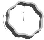
In Exp. (20) , $C_{order}$ represents how many times the wave length (𝜆) enters in a circumference perimeter of radius R . The tangential direction is the infinite direction in which the wave propagates in the analyzed structure. Notice that the relation between the wave number and the wave length is presented in the Exp. (5) . With the aim to illustrate the meaning of the Exp. (20) in Fig. 7 the ring with a $C_{order}$ = 8 is presented.

Figure 7
Axisymmetric model with $C_{order}=8$ .

To obtain the dispersion curves using the present methodology a scan of the band of the wave lengths of interest must be done. If we want to increment the value of the wave number k, the value of $C_{order}$ must be increased by decreasing the wave length $\text{λ}$ . For each value of $C_{order}$ the modal analysis computes the natural frequencies so that each one belongs to one propagating mode of the guided wave, in other words, it is a dispersion curve.

The possibility to compute the natural frequencies in axisymmetric models for a selected wave length is usually found in commercial codes of Finite Element Method, for example ANSYS, ( Ansys 2009 ) and ABAQUS,( Abaqus (2001) ).

In the present work, the commercial package based on FEM, ANSYS (2009) was used, applying the MODE command to define the parameter $C_{order}$ . More details about the way to determine points in the dispersion curve, using this methodology, can be found in Cegla(2008) . In section 5 of the present work the dispersion curve computation using this method for a rectangular bar will be presented.

4.2 The Computation of Dispersion Curves using a FEM tridimensional (Method 2).

In this circumstance, the methodology consists in carrying out the modal analysis using a FE tridimensional model applying periodic boundary conditions in the frontiers located in the wave direction (face A and B in the detail of Fig. 8 ). The periodic boundary conditions applied have the property to transform the tridimensional model in a portion of the guided wave, because the boundary conditions enforce that the two frontiers have the same displacement in magnitude and directions but in the opposite way. The wave length $\text{λ}$ could be expressed as it is indicated in Exp. (21) .

$\lambda =\frac{L}{p},$ (21)

where L is the model length (an arbitrary value that could be appropriately selected according to the range of interest in terms of wave length in the dispersion curve domain) and p is the quantity of spatial cycles that enter into de length FEM model. In practice, the determination of the number p depends on a visual analysis for each mode computed. In this way, it is possible to determine the points of the dispersion curves in the guided waves of interest. The aim of the method consists in enforcing the model through the boundary conditions applied to emulate a wave guide when mechanical waves cross the model.

Figure 8
Rectangular stem portion, detail about how the boundary conditions were applied.

The greatest advantage of this methodology consists in the possibility to visualize the propagation mode in a tridimensional model. The disadvantage is the difficulty to automatize the process of computing the dispersion curves points ( $\omega ,k$ ), due to the fact that the p constant must be determined by visual inspection.

More details about this methodology are found in Sorohan et. al. (2011) . In the present work the computational implementation of this method in the commercial FEM Package ANSYS, (2009) is built. The Exp. (22) , shows the kind of periodic boundary condition that must be imposed between the A and B model faces (see Fig. 8 ). CE is a ANSYS command that allows the application of this kind of boundary conditions.

${\displaystyle \sum }_{i=1}^n\left(u_{Aj}^i{C}_A+u_{Bj}^i{C}_B\right)=0.$ (22)

In the Exp. (22) , ${\text{u}}_{\text{Aj}}^{\text{i}}$ e ${\text{u}}_{\text{Bj}}^{\text{i}}$ are the displacements in the faces A and B. ${\text{C}}_{\text{A}}$ and ${\text{C}}_{\text{B}}$ are the scalar coefficients that determine the characteristics of this restriction. Fig. 8 also shows how the restrictions are imposed.

4.3 The determination of the dispersion curves using the Finite Element Method in the transversal section domain and the harmonic function in the wave guide direction (Method 3).

The present methodology consists in proposing a solution for the displacement field u, using the following Exp. (23)

$u=U\left(x_2,x_3\right)e^{\sqrt{-i^2}\left(k{x}_1-\omega t\right)},$ (23)

where $u$ represents the displacement vector, $k$ is the wave number, $\omega$ the circular frequency, $x$ the spatial coordinate, $t$ the time and $U$ represents the displacement amplitude in the transverse direction of the guided wave. Exp. (24) represents the Cauchy equation, that governs the static equilibrium in the $\Omega$ domain.

$C_{ijkl}\frac{{\partial }^2{u}_j}{\partial x_k\partial x_l}+\rho {\omega }^2{u}_i=0in\Omega$ , (24)

${\sigma }_i=C_{ijkl}\frac{\partial u_j}{\partial x_l}{n}_{k}on\Gamma$ , (25)

with $i,j,k,l=\mathrm{1,2,3.}$

The second term of Exp. (24) , in its original form, represents the body forces, but this version of the equation considers the product between the displacement vector and the square of the frequency. This form allows applying the methodology here described. In Exp. (25) the stress ${\sigma }_i$ over the boundary $\Gamma$ (mechanical boundary conditions) are shown, $n_k$ represents the components of the normal vectors to the body frontiers. Substituting the Exp. (23) in (24) and (25) it is obtained an equation system that could be solved as a quadratic eigenvalues problem.

It is possible to apply the present method in commercial FEM package that has the capacity to solve generalized eigenvalues problems. In the present work the software COMSOL(2012) was used. This software solves the equation

$-\lambda d_a\overline{U}+\nabla \left(-c\nabla \overline{U}+\alpha \overline{U}\right)-{\beta }_1\nabla \overline{U}-a\overline{U}=f$ , (26)

where $d_a,c,a,f,\alpha ,{\beta }_1$ represents a matrix of coefficients that permit the adaptation of the eigenvalue general problem to the specific problem associated to the Exp. (26) . 𝜆 represents the vector of eigenvalues, $\overline{U}$ represents the eigenvector matrix associated to the respective eigenvalue and $\nabla$ represents the Nabla differential operator. In the boundaries the Neumann condition is applied:

$-n\left(c\nabla \overline{U}+\alpha \overline{U}\right)=0$ , (27)

where $n$ represents the vector normal to the boundary, in each point of it. The expression (26) is solved for different values of $\omega$ , in this case the eigenvalues found will be wave numbers associated at the frequencies $\omega$ selected. In this way the curve of dispersion is made for the studied geometry. Details about the methodology here described are found in Predoi et. al. (2007) . The $d_a,c,a,f,\alpha ,{\beta }_1$ matrix of coefficients can be found in the appendixt C of Groth (2016) , for the isotropic case.

5-The case studied: The determination of the curves for a rectangular metallic rod.

As was indicated in the introduction, the interest in this particular geometry is linked to the fact that a similar structure is a component of the flexible risers, i.e., flexible piping employed to connect oil wells in the sea floor to the oil platforms. Through the methods presented in section 4, the dispersion curves are determined for the frequencies range ( $f$ [0, 100000] [Hz]) illustrated in Fig. 9 . The section of the guided wave studied is rectangular with 15x5 mm, with the properties of Carbon Steel ABNT 1020 ( ABNT NBR NM 87, 2000 ), with Young Modulus 200 [GPa], Density 7860 [Kg/m³] and Poisson coefficient 0.3).

Figure 9
Dispersion curve (a) in terms of frequency vs wave number.(b) in terms of the phase velocity vs frequency. The displacement fields associated with the modes in the points ( $a\omega$ , $b\omega$ , $c\omega$ , $d\omega$ ) were presented in Fig. 11 .

The four modes that appear in the bar of frequency indicated in Fig. 6 are: (a) the longitudinal mode (analogous to the mode S0 that appears in plates, illustrated in Fig. 6 (a, b)); (b) Bending Mode around the $x_2$ axis (analogous to the SH0 mode in plates); (c) the torsion mode that does not have the analogous in plates and finally (d) the bending mode around the $x_3$ axis (analogous to the plate mode A0 illustrated in the Fig. 7 (a, b)).

In higher frequencies, the dispersion curves increase in quantities and their drawing becomes complex. Examples of dispersion curves of rectangular bar in wide frequency domain can be found in Cegla (2008) .

In Fig. 9 a. the curves (a) and (c) represent the longitudinal and torsional propagation modes. The propagation velocity of these modes can be computed with Exp. (19) , that for the analyzed rectangular bar are $c_L=5043$ [m/s] and $c_T=1793$ [m/s].

In Fig. 9 b is verified how the dispersion curve associated with the longitudinal wave mode, curve (a) in Fig.9 a, is plotted in terms of the phase velocity vs frequency. This curve appears as a horizontal line that cuts the ordinate axis, in $c_L=5043\left[\text{m}/\text{s}\right]$ . On the other hand, curve (c), in Fig.9 a, correspond to the torsional wave mode and appears as a horizontal line that cuts the ordinate axis in $c_T=1793$ [m/s] in the Fig. 9 b.

This result indicates that a longitudinal perturbation, that propagates at any frequency, will travel in the stem always in the same propagation velocity $c_L$ . In other words, there is no dispersion in the longitudinal waves that propagates in a rectangular stem with this velocity. The same reasoning is possible with the torsional waves.

Notice in Fig. 9 b. that curve (a), strictly speaking, presents a slight declivity in a dispersion curve that could be explained for the lateral inertial effect presented in this kind of structures, Graff (1975) . In the case of the dispersion curve of torsion (curve (c)), in Fig. 9 b, also presents a little dispersion due to the influence of the warping in the transversal section of the guided wave studied. This effect is responsible for the coupling between the bending and torsion in this kind of sections. When the transversal section is tubular, it does not produce warping and for this reason the torsional mode does not present dispersion. Using this characteristic, the torsional waves are used in the inspection of rigid pipping, Rose (2014) . In Fig. 9 also the Curves b and d presented a great dispersion for low frequencies, but this dispersion effect diminished sensibly when the frequencies increase. These curves are linked with the bending modes around the axis 2 and 3.

In Fig. 10 , the same results shown in Fig 9 are presented in other domains. That is, wave length vs frequency, Fig.10 a, and group velocity vs frequency ( Fig.10 b). Notice that the difference between the phase velocity ( Fig.9 b) and the group velocity ( Fig 10 b) is a measure of the dispersion that presents each mode wave in the dispersion curves.

Figure 10
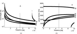
Dispersion curves (a) in terms of wave length vs frequency. (b) of group velocity vs frequency.

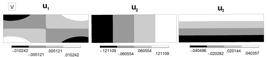
In Fig. 11 the mode shape is presented in the three orthogonal directions for the four wave modes of the dispersion curves a, b, c, and d plotted in Fig.9 and 10 . These fields were determined for the frequency of 50 [kHz], that present the wave modes, which correspond to the points indicated as a$\omega$ , b$\omega$ , c$\omega$ , d$\omega$ in Fig. 9 a.

Figure 11
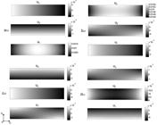
The modal displacement for the wave modes linked with the curves a,b,c,d, at the frequency of 50KHz.(see Fig. 9 ). Here the axis $x_2$ and $x_3$ are in the transversal section of the guided waves considering $x_1$ , in the guide propagation direction. The modal displacements were obtained using the Method 3, described below.

The mode that correspond to the point a $\omega$ over the dispersion curve (a) have a displacement in the longitudinal direction higher than the displacement field in the other orthogonal directions. Also notice that, in analogy with the wave propagation in plates related to the neutral longitudinal plane( $x_{\mathrm{1,}}{x}_3$ ), there is symmetry in the displacements $u_1$ and antisymmetry in the displacement $u_2$ , the same behavior is presented in the characteristic wave mode of S0 in the plates (see Fig. 7 ).The displacement fields linked with the point d$\omega$ are associated with a bending mode related to the $x_3$ axis and presented in Fig.11 . In this situation, the displacement $u_2$ is symmetric and the displacements $u_1$ are antisymmetric related to the horizontal neutral plane ( $x_{\mathrm{1,}}{x}_3$ ). The same characteristics appear in the plate mode A0 (see Fig. 7 ). The fact that the displacements $u_2$ are higher than the other displacement, in this mode, characterizes the bending in respect to the axis $x_3$ . The mode associated with the point c $\omega$ over the dispersion curves presents a typical shape of torsion. The displacement $u_1$ distribution allows to understand the coupling between bending and torsion. In this mode shape the fields increase from the center to the borders of the transversal section.

5.1 Comparison among the methods to compute the dispersion curves:

Following the three methodologies presented in section 4 to determine the dispersion curves of a metallic rectangular stem, curves were computed with the method 3. For the specific wave number (k=50 [1/m]) equivalent to $\lambda =2\pi /k=$ 0.1256 [m] the values of the dispersion curves were computed in a frequency interval of [0,50]kHz. The four points indicated in the Fig. 12 were obtained using the other two methods.

Figure 12
Dispersion curves are indicated by the points ak, bk, ck and dk computed with the first method.

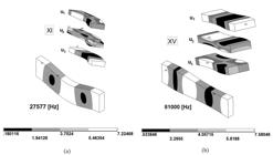
Notice the good agreement among the semi-analytical methods presented in table 1 for the points indicated as ak, bk, ck, dk in Fig. 12 . The torsional wave mode associated with the point ck was computed with the Method 2 and is shown in Fig.13 . Using Method 1 the results in terms of the configuration Mode in Fig. 14 . The figures show the similarity between the modes computed with the different methodologies. The mode in the point cω, presented in Fig. 9 and 10 computed with the Method 3 is shown in Fig. 11 . This mode is over the curve c, close to the point ck and the shape of both modes are similar as it is possible to observe comparing the Figs. 13 and 14 .

Table 1
Comparison among the Methods 1, 2 and 3.

MODES (k=50 [1/m])	Frequency [Hz]
	Method 3	Method 2	Method 1
Dk	2,862	2,957	2,884
Bk	8,333	8,232	8,030
Ck	14,313	14,487	14,197
Ak	41,539	41,210	40,539

Figure 13
Mode associated with the point ck depicted in Fig.12 , computed with Method 2. In the detail the displacement is presented. This modal configuration also corresponds to the point identified as (V) in the Fig.15 . (In this case, p=0.5 is the number of the length wave that enters in the stem portion investigated, that has a length of L=0.0628m).

Figure 14
Mode linked to the point ck, depicted from Fig. 11 , was computed using the Method 1 considering $R=50\left[m\right]\text{and}{C}_{order}=2500$ . Then λ=2πR/C_order=0.1256m, and k=2π/λ=50 m. The modal displacement $u_2$ , according to the results obtained with the others methods, is the highest component. This modal configuration also corresponds with the point identified as (VI) in the Fig.15 .

In Method 1 the domain with 4-nodes axisymmetric quadrilateral elements is used. This element is described in Zienkiewicz(1977) . In the ANSYS environment(ANSYS2009) this element is called PLANE25. The element characteristic size used was 0.2mm. Therefore, the bar rectangular section of 5x15mm was discretized by 25x75 elements.

Method 2 was also implemented in the FE commercial package ANSYS. In this case, 8 node brick element was used, as described in Taylor et al. (1976) and called SOLID45 in the ANSYS environment (ANSYS2009). In this case, the element characteristic size was 0.8mm, so 6x18 elements, to discretize the transversal section, were used. In the longitudinal direction, we consider that the shortest wave length modeled correspond to k=350 (see Fig. 9 and 10 ), so the shortest wave length modeled corresponds to λ=2π /350=22.5mm, therefore, close to 28 elements were used to model the shortest wave length.

In method 3 the spatial domain with three nodal triangular element with largest characteristic size of 0.3mm was used. The description of this element is found in COMSOL 2012. In this case the transversal section was discretized with 18x50 elements. A discussion about the level of discretization used in all the simulations will be presented in the conclusions.

The advantage of Method 2 to understand the mode shape is evident. In the detail of Fig. 13 one can notice where the maximum displacement in each direction happens, and it is possible to perceive that the maximun displacement does not happen in the same transversal section.

In Fig.15 the dispersion curves of the rectangular bar obtained with Method 3 were indicated and over the same curves the points that were computed using the Methods 1 and 2 were identified with roman numbers. The modes configurations obtained in these points are presented in Figs. 16 - 19 . In this way, the three methodologies validation that computed the dispersion curves were done and also illustrate better the information that these curves enable to obtain.

Figure 15
The Dispersion Curves were computed with the Method 3. Over these curves, points where the wave modes were computed, using the Methods 1 and 2, are presented in the Figs. 16 - 19 .

Figure 16
The configuration evolution computed with the Method 2. On the dispersion curve c (torsion). The same L and different values of p.

Figure 17
Three configuration modes on the dispersion curve d (see Figs.9 and 14 ), bending mode around the $x_3$ axis . Configurations computed with the Method 2. Perceive that in mode XIII auxiliary lines indicate that in this case the wave enters 2.25 times in L=0.0628m, that is p=2.25.

Figure 18
(a)The mode configuration on the curve b (see Figs.9 and 15 )(A bending mode around the $x_2$ axis), (b) The mode configuration on the curve a(see Figs. 9 and 15 )(A longitudinal Mode). In both cases it was used the method 2 with k=100m^-1 and p=1.

Figure 19
Displacement fields obtained with the Method 1 adopting $R=50\text{and}{C}_{order}=\mathrm{2,500}$ . (equivalent to k=50 m^-1).

In Fig. 16 4 modal configurations (I, II, III, and IV) are presented, computed with the Method 2, and identified over the dispersion curves presented in Fig. 15 . These configurations present a clear dominant torsion in their shape. Notice that these points are on the curve c in Fig. 9 a and b. It is also observed in these configurations that when the wave number increases the shape of the configuration changes. In the configuration represented in point (I) the wave number will be k=100. As the prism length modeled with Finite Element Method using the Method 2 is L=0.0628m, in this case it enters in such length only one wave length, because in this one (𝝀=2π/k= 2π /100=0.0628m), in this circumstance p=L/ 𝝀 =1. For the other configurations (II, III, IV) there will be higher values of p. Using the same argument in the point (VI) p=0.0628m/0.1256m=0.5.

In Fig. 17 the modal configurations associated with bending around the axis ${\text{x}}_3$ are presented. This mode is analogous to the one presented in a plate, called in this case A0 mode by Auld (1973) . In this situation the configurations (X, XII, XIII and XIV) are presented. Notice that for the configuration XIII the value of p=2.25 corresponds, as shown in Fig. 16 , to the wave number k=225m^-1. In Fig. 17 for configuration XIII we added auxiliary lines to perceive better that the wave length enters 2.25 times in the bar length of L=0.0628m.The four modal configurations presented are on the curve d, (see in Figs. 9 and 15 ). It is also possible to compare the shape of these configurations. See, for example, the configuration IX computed with the Method 1 presented in Fig. 19 , notice that this mode is a bending around the axis x₃ .

Fig. 18 presents the configuration XI computed with the Method 2, this configuration is on the curve b presented in Fig. 9 and is characterized as a bending with respect to axis x2. In Fig. 18 the configuration VIII is presented using the Method 1 and using another wave number. In this configuration mode the bending around the x2 axis appears as dominant.

In Fig. 18 also computed employing the Method 2, the configuration XV is shown. There the longitudinal mode predominates. As it is illustrated in Figs. 9 and 15 , this configuration is on curve a. It is also possible to compare configuration XV with configuration VII computed with the Method 1 presented in the Fig. 19 . It is possible also to observe that the two configurations present similar shapes for the modal displacement fields.

6 Numerical Verification: Analysis of prismatic bar submitted to longitudinal and transversal excitation.

Aiming to verify the dispersion curves presented in previous sections, the simulation of specific wave propagation in a prismatic bar of 1500x15x5mm was used. The simulation was made using the LSDYNA (2003), a FEM commercial package that is characterized by making the integration in time domain of the motion equation that governs the mechanical vibration of this kind of structures, using an explicit scheme of integration. In the LSDYNA environment a hexaedral Solid Element, implemented in the LSDYNA element library, was used. More details about this element could be found in Flanagan and Belytschko (1981) . In this case, the elements used have a characteristic size of 1mm. Then the transversal section was discretized by 5x15elements. In the longitudinal direction, the shortest wavelength that was discretized corresponds to a wave number of 250. Observe in Figs. 9 and 10 that, linked with an excitation frequency used in this simulation (50 kHz), the wave number associated with this frequency is k=220. That is, the shortest wave length needed to be modeled is λ=2π/220=28.5mm, then around 28 elements were used for simulation of the shortest wave length. A discussion about the level of discretization used will be presented in the conclusions.

The model was excited as a Hanning windowed function, also called Tone Burst function, described by Rose (2014) . This function consists in a harmonic function modulated with other harmonic function with lower frequency or other envelopment function such as a Gaussian Function. This function is a perturbation with a defined frequency band. In the model a Tone Burst was applied with 50KHz modulated with another harmonic function with a frequency of 10KHz. In this way only 5 waves enter into the envelopment with the frequency of 50KHz.The excitation is presented in the detail of Fig. 20 .

Figure 20
The numerical analysis of the excitation tone burst of 50KHz and five cycles over a metallic rectangular stem. The black arrow indicates the direction and region where the force was applied. The transversal views show displacement and they are done in the time when the wave passes through the transversal section of the stem. The images were extracted in the simulation in the time instant t = 0.275 [ms].

In Fig. 20 it is also illustrated that the Tone Burst wave used excites the wave modes identified in the dispersion curves. These are presented in Fig. 9 around the points a$\omega$ and d$\omega$ when the excitation has the longitudinal direction and around the points c$\omega$ and b$\omega$ when the excitation has the transversal direction. This fact becomes evident when comparing the displacement map presented in Fig. 20 with the modal configurations presented in Fig. 11 . Fig. 20 illustrates that the component of the excitation linked with the configuration mode a $\omega$ is faster than the displacement component linked with the mode configuration d $\omega$ . This information is consistent with Fig.9.b where the phase velocity associated with the wave mode a$\omega$ presents a higher velocity than the wave mode d$\omega$ .

Similarly, when the transversal excitation is applied, as illustrated in Fig. 20 the wave mode b$\omega$ is faster than the wave mode c $\omega$ (at 50 [kHz]). The way as the excitation applied is decomposed in the mode waves that propagate in different group velocities could help in the damage detection techniques because, in this case, the structure causes a natural decomposition of the applied excitation.

7 Experimental validation

With the objective of validating the numerical results, here presented, experimental tests were carried out. In these tests, the same problem described in section 6 were made. It was considered a metallic rectangular bar with dimension 5x15x1500mm built with Carbon Steel ABNT 1020 ABNT NBR NM 87 (2000) (Young Modulus 200 [GPa], Density 7860 [Kg/m³] and Poisson coefficient 0.3).

The wave modes were excited in the same way it was indicated in section 6, that is, with a Tone Burst force excitation. This type of excitation, as explained in Rose 2014, is built with a Hanning window, with a central frequency of 50KHz. The ceramic vibration excites the body test and this perturbation propagate in the bar as a guided wave. The transductors used in the excitation were two piezoelectric ceramic, Ferroperm (2016) , with dimensions of 1x3x13[mm], stuck in the body test surface with an epoxy resine.

Sensors with different polarizations were used to apply longitudinal and transversal excitatiogons. The excitation is produced applying a potential difference over the transductors by means of a function generator Agilient, 33521A, Keysight (2016) . Also, in the excitation system a tension amplificator Krohn-Hite 7500, Krohn-Hite (2016) is used. The waves travel on the body test and a laser vibrometer registers the velocities in the selected directions, Castellini et al (2005) . The velocities over the different points on the surface body test are collected with two vibrometers model OFV-505, Polytec (2016) . These sensors are linked with the controller and data acquisition system NI PXIe-1062Q, ( National NI, 2016 ). This system digitalizes the measures captured by the vibrometers and saves this information in ASCII text format. The data are processed using a Desktop with the following configuration: PC Lenovo® with a processador of 3.30 GHz Intel ® and 8 GB of RAM Memory using in the software MatLab ® (2016).

The Fig. 21 shows a scheme with the experimental components set up.

Figure 21
Experiment set up scheme.

The velocity of one point on the surface specimen is captured by the vibrometers. The vibrometers lay out is presented in Fig 22 . This system measures the movement in a plane where the ceramic PZT is fixed . Using a configuration of two sensors it is possible to know if the velocity is in or out of the propagation plane by means of the phase analysis of the signals produced by the sensors. If the signals are in phase, then the movement will be out of the propagation plane. If the one signal is positive and the other is negative, that is, the phase is 180^o, then the movement will be in the propagation plane. The Laser vibrometer is an ideal sensor to capture the wave propagation because it gets the signal with high spatial and temporal resolution and the measurement system does not interact with the wave propagation therefore, the propagation is not perturbed by the system ( Barker (1972) ). Using this set up the experimental verification is made.

Figure 22
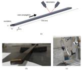
Experimental layout, (a) General scheme where the position of the laser vibrometer is fixed to measure a wave that propagates in the bar b) The ceramic pzt stuck in the specimen and c) The Polytec laser vibrometers.

The end of the specimen on the superior surface is in ideal position to apply a surface excitation, because the PZT ceramic with transversal polarization, that is, in the axis (3) direction, produces a torsion and bending around the axis (2). Using the same logic, the polarization in the longitudinal direction, that is in the axis (1) direction, produces a longitudinal and a bending around the axis (3) waves . With these two configurations of coupling and polarization, the four fundamental modes of a rectangular wave guide are excited, that is: longitudinal, torsional and bending around the axis (2) and (3).

To validate the model with the transversal excitation an acquisition of the instantaneous velocity on one point is done . This point is situated on the surface at 1m from the excitation source was applied. The comparison between the experimental results and the results obtained using the numerical model, presented in the section 6, are shown in the Fig. 23 . The magnitudes of the results were normalized because in the present case the focus is verified if the modes excited during the propagation in the test and in the simulation are similar.

Figure 23
Results in terms of the velocity in the dir 3 due to the transversal excitation applied (a tone burst function with a central frequency of 50KHz). Torsional and bending wave respect with the axis 2 appear in the plot. The point, where the response is measured, is situated at 1meter from the excitation applied. Experimental result in continuous line, Numerical result in discontinuous line.

It is also observed, in Fig. 23 , that the application of transversal Tune Burst excitation with a main frequency of 50KHz excites two wave modes, a flexural mode respect with axis 2 and a torsional wave mode. These two modes propagate with different velocities. Then, the results presented in Fig.23 are coherent with the simulation presented in Fig.20 (a) and with the dispersion curves presented in Figs. 9 and 10 . Also a longitudinal excitation using a piezoelectric transductor was applied, but with different polarization to excite the specimen with a longitudinal wave. In the present case, results, in terms of instantaneous velocity in the dir. 1, are captured on the surface with distance of 1.5m from the position where the excitation was applied. In Fig. 24 the experimental and the numerical results obtained with the model are shown.

Figure 24
Results in terms of the velocity in the dir. 1 due to the longitudinal excitation applied (a tone burst function with a central frequency of 50KHz). Axial and bending wave modes around the axis (3) appear in the plot. The point, where the response is measured, is found at 1.5meter from the excitation applied. Experimental result in continuous line, Numerical result in discontinuous line.

In the second experiment, the longitudinal harmonic excitation applied in the bar surface with main frequency of 50KHz was also observed activating mainly a longitudinal mode (fastest mode) and a bending mode around the axis (3). In this case the velocities of two modes are higher than in the first test, for this reason the highest possible distance between the excitation source and the point, where the measure is carried out, was adopted. So all the length bar (1.5m) was used to avoid that the wave reflection appearing in Fig. 24 .

The experimental propagation velocities, in terms of time and distances, are in accordance with the numerical results obtained in section 6,( Fig 20 (b)). It is also possible to see that the experimental verification is in accordance with the dispersion curves computed in Figs 9 and 10 in Section 5.

8 CONCLUSIONS

In the present work the behavior of a guided wave with a metallic stem with rectangular section was studied. The computation of the dispersion curves was carried out in a frequency interval of [0,100KHz] for the same structure. Three methodologies to compute the dispersion curves were used.

An effort was done to apply the three methodologies to explain physically the guided wave behavior.

The stem response against the Tone Burst excitation was simulated making the link between the dispersion curves, associated with the specific stem geometry, and the process of dispersion of the excitation applied. Finally, also was carried out an experimental verification with the aim to assess the quality of the numerical simulations. During the work it was possible to conclude that:

• It was taken as premise to present the concept related with wave guide in the simplest way possible, to turn the present paper easy to understand for non specialized community in the wave propagation topics.

• The three methodologies applied to compute the dispersion curves in the metallic stem presented coherence .

• In all the Finite elements models used, the level of discretization was enough to obtain good results, according to Marburg & Nolte (2008) . In the cited bibliography, the shortest wavelength discretized is recommended as at least 6 elements. For instance, in the method 2, 18 elements were used for the shortest wave length and in the numerical verification, presented in section 6, 22 elements for the shortest wave length were used. In the transversal section, the criterion to consider that each characteristic length as equivalent to a semi length wave was adopted. Up to this criterion, the minimum dimension was discretized by 25 elements in method 1. In method 2 and 3 by 18 elements and in the verification method the minimum dimension was discretized by 5 elements.

• With the aim to evaluate the performance of the SAFE method, here presented, it is necessary to compare the methods with equivalent level of discretization. In the present work this comparison was not done, only a discretization level to guarantee good results was used in all models. The comparison among them was done taking into account other aspects, for instance: automatization, method facilities, and the mode visualization characteristics.

• The three SAFE Methods presented coherence when applied in the construction of the dispersion curves of a bar with rectangular section guide wave in the frequency interval [0,100KHz]. Method 1 presented the advantage of implementation, simplicity and low computational cost. Method 2 presents the advantage to see the mode in three dimensions. Method 3 has a strong quality that, in this case, is easy to implement the automatic generation of the dispersion curves. The software where method 3 is implemented in COMSOL 2012 that interact with the software Matlab(2016) with extremely facility.

• In the three implementations, commercial finite element packages are accessible to engineers without a specific knowledge in solid wave propagation.

• The displacement fields, obtained by the SAFE methods, were validated using the numerical model, presented in section 6, where the commercial package LSDYNA(2003) was used to represent the propagation of a Tone Burst excitation in the bar and to map which wave mode will be activated. It was possible to verify that the results obtained were coherent with the dispersion curves obtained.

• In the computation of the dispersion curves of the wave guide with one infinite dimension, for a low frequency interval, four basic wave modes always appear: axial, torsional and wave modes related to bending respect with two transversal axis. In the case studied this premise was verified.

• The simulation of the Tone-Burst excitation in the bar also allows to verify the crucial role of the dispersion curves to understand the decomposition of the excitation, in the mode waves.

• In the experimental study the results presented coherence with the numerical verification made and indirectly, the dispersion curves obtained with the three methodologies proposed were validated.

• Finally, notice that the simulation of waves propagation in guided waves, allows to understand better the phenomena studied and help the tests interpretation that could be made in the context of nondestructive techniques, based on the guided waves propagation.

Acknowledgment: We would like to thank CNPq (National Council for research in Brazil) for the financial support.

• http://dx.doi.org/10.1590/1679-78254527

References

• 4subsea <https://www.4subsea.com/solutions/flexible-risers/structural-assessment/>access jan 2018.
  » https://www.4subsea.com/solutions/flexible-risers/structural-assessment/
• Aalami B., (1973) Waves in Prismatic Guides of Arbitrary Cross Section. Jornal of Applied Mechanics. 1067:1072
• Abaqus (2001). User’s Manual. Hibbitt, Karlsson&Sonrenses, Inc. (Boston).
• Åberg, M. and Gudmundson, P.,(1997). “The usage of standard finite element codes for computation of dispersion relations in materials with periodic microstructure”. J. Acoust. Soc. Am. 102 (4), pp. 2007-2013.
• ABNT NBR NM 87(2000). ‘Carbon steel and alloy steel for general engineering purpose - Designation and chemical composition´.
• Ansys.(2009). Structural Analyses Guide, ANSYS, Inc. (Canonsburg).
• Auld B. A., (1973). Acoustic Fields and Waves in Solids, John Wiley and Sons (New York).
• Barker L. M. (1972). Laser Interferometry in Shock-wave Research. Exp Mech 12:209-215 doi: 10.1007/BF02318100
  » https://doi.org/10.1007/BF02318100
• Bartoli I., Marzani A., Matt H., di Scalea F. L., (2006) Modeling wave propagation in damped waveguides with arbitrary cross-section.Proc. Of SPIE 6177: 61770A1-12.
• Banerjee S., Kundu T., (2006). Symetric and anti-symmetric Rayleight-Lamb modes in sinusoidallyconrrugated waveguides: An analytical approach. International Journal of Solids and Structures. 43:6551-6567.
• Barnwell E. G., Parnell W. J., Abrahams I. D. (2016). Antiplane elastic wave propagation in pre-stresses periodic structures; tuning, band gap switching and invariance. Wave Motion, 63:98-110.
• Barnwell E. G., Parnell W. J., Abrahams I. D.(2017). Tunable elastodynamic band gaps. Extreme Mechanics Letters, 12:23-29.
• Castellini P., Martarelli M., Tomasini EP., (2005). Laser Doppler Vibrometry: Development of advanced solutions answering to technology’s needs. Mechanical Systems and Signal Processing. DOI 10.1016/j.ymssp.2005.11.015.
  » https://doi.org/10.1016/j.ymssp.2005.11.015
• Castaings M., Bacon C., (2006).Finite element modeling of torsional wave modes along pipes with absorbing materials.Jornal of Acoustic Society of America 119:3741-3751.
• Cegla F. B., (2008). Energy concentration at the center of large aspect ratio rectangular waveguides at high frequencies. Journal of Acoustic Society of America 123: 4218-4226.
• Comsol (2012). COMSOL Multiphysics User’s guided, COMSOL 4.3.
• Costa, C. H. O., Roitman, N.,Magluta, C., Ellwangwer, G. B., (2003). Caracterização das propriedades mecânicas das Camadas de um RiserFelxível, 2° Congresso Brasileiro de P&D em Petróleo & Gás (Rio de Janeiro).
• Chree, C., (1889) The equation of an isotropic elastic solid in polar and Cylindrical coordinates, their solution and applications. Transactions of the Cambridge Philosophical Society 14: 250-369.
• Demma, A.; Cawley, P.; Lowe, M.; Roosenbrand, A.G.; Pavlakovic, B.(2004); “The reflection of guided waves from notches in pipes: a guide for interpreting corrosion measurements”, NDT&E International 37, p167-180.
• Duan W., Kirby R. (2015). A numerical model for the scattering of elastic waves from a non-axisymmetric defect in a pipe . Finite Elements Analysis and Design 100. 28–40
• Ferroperm,(2016) Piezoceramics catalogue. Available in http://www.ferroperm-piezo.com/files/files/Ferroperm%20Catalogue.pdf found at September 6 2016.
  » http://www.ferroperm-piezo.com/files/files/Ferroperm%20Catalogue.pdf
• Flanagan, D. P. and Belytschko,T. (1981), ‘ A Uniform Strain Hexahedrom and Quadrilateral and Orthogonal Hourglass Control.’Int. J. Numer. Meths. Eng. 17, 679-706.
• Glushkov E., Glushkova N., Fomenko S. (2017) . Wave generation and source energy distribution in cylindrical fluid-filled waveguide structures. Wave Motion Journal. Vol72:70-86.
• Golgoon A.,Yavari A. (2017).On the stress field of a nonlinear elastic solid torus with a toroidal inclusion. Journal of Elasticity, 128(1):115-145.
• Golgoon A., Yavari A.(2018). Nonlinear elastic inclusions in anisotropic solids. Journal of Elasticity, 130 (2):239-269.
• Golgoon A., Sadik S., Yavari A. (2016). Circumferentially-symmetric finite eigenstrains in incompressible isotropic nonlinear elastic wedges. International Journal of Non-Linear Mechanics, 84:116-129.
• Graff K. F., (1975). Wave Motion in Elastic Solids, Dover Publications (New York).
• Gavric L., (1994). Finite element computation of dispersion properties of thin walled waveguides. Journal of Sound and Vibration, 173 (1), pp. 113-124.
• Gavric L., (1995). Computation of propagative waves in free rail using a finite element technique. Journal of Sound and Vibration, 185 (3), pp. 531-543
• Groth E. B. (2016). Propagação de ondas de tensão em hastes retangulares no intervalo de frequência de (0;100 [kHz]). Master dissertation. UFRGS. http://www.lume.ufrgs.br/handle/10183/142694.
  » http://www.lume.ufrgs.br/handle/10183/142694
• Huang K. H. & Dong S. B. (1984). Propagation waves and edge vibration in anisitropic composite cylinders . Journal of Sound and Vibration. 96(3): 363-379.
• Lagasse P. E., (1973) Higher-order finite-element analysis of topographic guides supporting elastic surface waves. Journal of Acoustic Society of America 4:1116-1122.
• Keysight. 33521A Waveform Generator. (2016) Available in http://literature.cdn.keysight.com/litweb/pdf/5990-5914EN.pdf?id=1919803 found at September 12, 2016.
  » http://literature.cdn.keysight.com/litweb/pdf/5990-5914EN.pdf?id=1919803
• Krohn-Hite Model 7500 wideband power amplifier manual.(2016). Available in http://www.krohn-hite.com/htm/amps/PDF/7500%20Manual.pdf found at September 12.
  » http://www.krohn-hite.com/htm/amps/PDF/7500%20Manual.pdf
• Lamb H., (1916). On Waves in an Elastic Plate.Proceedings of the Royal Society of London. 93:114 – 128 (London)
• Li J. Y., Qiu Z. X., Ju J. S., (2014). Numerical Modeling and Mechanical Analyses of Flexible Risers.Mathematical Problems in Engineering.
• Ls-Dyna (2003). Theory Manual, Livermore Software Technology Corporation (California).
• Marburg, S., Nolte,B. (Eds.). (2008). ´Computational Acoustics of Noise Propagation in Fluids- Finite and Boundary Elements Methods., 578p. Springer Verlag. ISBN: 978-3-540-77447-1.
• MatLab, Getting Started(2016), Available in https://www.mathworks.com/help/pdf_doc/matlab/getstart.pdf found at September 6.
  » https://www.mathworks.com/help/pdf_doc/matlab/getstart.pdf
• Moore P. O., Miller R. K., Hill E. v.K. (2005). Acoustic emission testing, Nondestructive testing handbook, American Society for Nondestructive Testing.
• National NI PXIe-1062Q User manual (2016). Available in http://www.ni.com/pdf/manuals/371843d.pdf found at September 6, 2016.
  » http://www.ni.com/pdf/manuals/371843d.pdf
• Predoi M. V., (2014). Guided waves dispersion equations for orthotropic multilayered pipes solved using standard finite elements code. Ultrasonics 54:1825-1831.
• Predoi M. V., Castaings M., Hosten B., Bacon C., (2007). Wave propagation along transversely periodic structures. Journal of Acoustic Society of America 121: 1935-1944.
• Pochhammer L., (1876). Ueber die FortpflanzungsgeschwindigkeitenkleinerSchwingungen in einemunberenztenisotropenKreiscylinder. Journalfür die reine undangewandte Mathematik 81: 324-336. (Germany).
• Polytec, Vibrometer Controller datasheet. (2016) Available in http://www.polytec.com/fileadmin/user_uploads/Products/Vibrometers/OFV-5000/Documents/EN/OM_DS_OFV-5000_E_42346.pdf. found at September 6, 2016.
  » http://www.polytec.com/fileadmin/user_uploads/Products/Vibrometers/OFV-5000/Documents/EN/OM_DS_OFV-5000_E_42346.pdf
• Ramatlo D., Long C., Loveday P., Wilke D.(2016). SAFE-3D Analysis of a Piezoelectric Transducer to ExciteGuided Waves in a Rail Web. 42nd Annual Review of Progress in Quantitative Nondestructive Evaluation. AIP Conf. Proc. 1706, 020005-1–020005-10; doi: 10.1063/1.4940451. AIP Publishing
  » https://doi.org/10.1063/1.4940451
• Rose J.L. (2014) Ultrasonic guided waves in solid media. Cambridge University Press, New York.
• Royer D., Dieulesaint E., (1996). Elastic Waves in Solids I, Free and Guided Propagation, Springer (Paris).
• Simonetti F., Cawley P., (2003). A guided wave tchnique for the characterization of highly attenuative viscolastic materials. Journal of Acoustic Society of America 114: 158-165.
• Shearer T., Parnell W. J., Abrahams I. D. (2015). Antiplane wave scattering from a cylindrical cavity inpre-stressed nonlinear elastic media. Proc. R. Soc. A, 471(2182):20150450.
• Sorohan S., Constatin N., Gavan M., Anghel V., (2011). Extration of dispersion curves for waves propagating in free complex waveguides by standard finite element codes. Ultrasonics 51: 503:515.
• Taylor R. L., Beresford P. J., Wilson E. L. .(1976). “A Non-Conforming Element for Stress Analysis”. International Journal for Numerical Methods in Engineering. Vol. 10. 1211-1219.
• Wilcox P., Evans M., Pavlakovic B., Alleyene D., Cawley P., Lowe M., (2003). Guided wave testing of rail. NDT & E Insights Vol 45: 413-420.
• Wilcox P., Evans M., Diligent O., Lowe M., Cawley P. (2002). Dispersion and excitability of guided acoustic waves in isotropic beams with arbitrary cross section. API Review of Nondestructive Evaluation Vol. 21. 203-210
• Zienkiewicz O. C. (1977). The Finite Element Method. McGraw-Hill Company. London.
• Zuo P., Zhou Y., Fan Z.(2016) Numerical studies of nonlinear ultrasonic guided waves in uniform waveguides with arbitrary cross sections. AIP Advances 6, 075207; doi: 10.1063/1.4959005.
  » https://doi.org/10.1063/1.4959005

Publication Dates

• Publication in this collection
  02 July 2018
• Date of issue
  2018

History

• Received
  21 Sept 2017
• Reviewed
  26 Mar 2018
• Accepted
  31 Mar 2018