A mixed 3D-1D finite element formulation for analysis of geomaterial structures with embedded curvilinear inclusions: application to load transfer in mooring anchor systems

Abstract

A finite element model for structural analysis of media with embedded inclusions is presented. The “embedded element concept” is adopted to model the contact interaction of two medium components along the contact interface considering a mixed 3D-1D formulation. The Mohr-Coulomb interface model is employed to define the bond-stress and bond-slip relation and strains associated with bond-slip are assumed to remain infinitesimal along the interface. Nonlinear analysis is performed with a corotational kinematics description introduced in the context of embedded approach. The problem of load transfer in mooring anchor systems was investigated and reasonable results were obtained using the present model.

Keywords
embedded inclusion; bond-slip model interface; finite element modeling; embedded model; corotational kinematics

1 INTRODUCTION

Many problems of structural engineering as well as geotechnical and petroleum engineering involve linear or curvilinear inclusions embedded in a solid material matrix. Reinforced concrete is the most common example with reinforcing steel bars modeled as cable elements and incorporated into the finite elements referring to the concrete material (see for instance Manzoli et al. (2008), Oliver et al. (2008) or Figueiredo et al. (2013), to cite some recent references among the numerous contributions in the field). Similar approaches, such as those implemented by Zhou et al. (2009) or Maghous et al. (2012), may also be used in geotechnical applications, especially for load evaluations in anchoring systems employed in offshore oil platforms, where soil-mooring line interaction can be characterized using a mixed 3D-1D finite element formulation. In this case, the kinematic and constitutive descriptions of the interface phenomena play a key role.

It is underlined that when the medium consists in a homogeneous matrix reinforced by several linear inclusions that are arranged periodically, the homogenization method or multiphase modelling appear as alternatives to handling the matrix/inclusion interaction problem (see for instance Bernaud et al. (1995), de Buhan and Sudret (1999), Sudret and de Buhan (2001), Bennis and de Buhan (2003), Hassen and de Buhan (2006), de Buhan et al. (2008), Bernaud et al. (2009), Hassen et al. (2013), to cite a few).

Mooring systems are utilized in the offshore petroleum industry to maintain floating platforms attached to the exploitation site. A mooring system is basically composed by mooring lines and anchors, which is submitted to hydrodynamic and aerodynamic loads applied on the floating structure and transferred to the mooring lines through fairlead points located on the platform. Owing to friction forces developed along the mooring line, the load applied on the anchoring device is not the same as that observed on the platform. Taking into account that the mooring system depends totally on the strength of the anchor, dissipation produced by friction forces acting on the soil-cable interface along the buried segment of the mooring lines must be determined in order to properly evaluate the load applied on the anchoring device, considering that the friction forces acting along the line segment immersed in the sea water are determined. Previous works on this subject may be found in Degenkamp and Dutta (1989), Neubecker and Randolph (1995), Yu and Tan (2006) or Wang et al. (2010a, 2010b).

The structural response of one-dimensional structures immersed in a three-dimensional solid medium requires a special system. Although a numerical model based on contact mechanics for multibody systems can be adopted for the analysis (Wriggers, 2006; Laursen, 2010), the use of the so-called “embedded element concept” is much more efficient, considering that the diameter of the embedded one-dimensional structure is significantly smaller than the typical size of the surrounding solid. The embedded formulation was introduced by Phillips and Zienckiewicz (1976) to analyze concrete structures. Since then, improvements have been made regarding the description of mechanical behavior and search algorithms for localization of the reinforcement within the solid matrix. Chang et al. (1987) modified the original formulation in order to allow straight reinforcement elements embedded in arbitrary direction with respect to the local axes of the solid matrix element. Balakrishnan and Murray (1986) presented an embedded formulation with bond-slip interface, while Elwi and Hrudey (1989) extended the two-dimensional embedded formulation by using reinforcements with curved shape. Barzegar and Manddipudi (1994) proposed a general model for spatial modeling of straight segments of embedded reinforcement using inverse mapping and a search algorithm for intersection points between reinforcement and solid elements. Owing to the use of straight elements, a refined mesh is necessary in the matrix solid field in order to define reinforcements with curved shape. Ranjbaran (1996) proposed a numerical formulation for embedded reinforcements in 3D brick elements, where full bond between the solid matrix and reinforcement are assumed. Gomes and Awruch (2001) extended the search algorithm proposed by Barzegar and Manddipudi (1994) to account for curved elements embedded in hexahedral finite elements with quadratic interpolation functions. More recent works have improved the description of the solid-structure system including flexural rigidity in order to represent the one-dimensional structure using beam models, which can be utilized to simulate soil-structure interaction problems involving piles (e.g., Sadek and Shahrour; 2004; Ninic et al., 2014).

In the context of mixed 3D-1D formulation, special emphasis must be given to properly describe the interface phenomena. A Mohr-Coulomb interface model can be adopted to define the constitutive relationship between bond-stress and bond-slip, where an elastic-plastic formulation is utilized in order to define the bond-stress evolution based on the slip motion along the tangential direction of the interface, which may be reversible or irreversible. Unlike matrix and embedded inclusion, which may undergo large strains, the bond-slip is assumed to remain infinitesimal along matrix/inclusion interface. This assumption may be viewed as first approach to assessing the kinematical description of the relative motion on the interface. Clearly enough, a more comprehensive modeling is still to be developed in order to properly take into account large relative displacements along the interface.

In this context, it is noted that the objective of this contribution is to formulate a mixed 3D-1D finite element method for analyzing solid-structure interactions in geomaterials with embedded curvilinear inclusions. In terms of engineering application, the proposed finite element modeling is applied to evaluate the load attenuation at the anchoring point of a typical mooring line utilized in anchoring systems of offshore platforms, considering the solid-structure interaction occurring along the buried segment of the mooring line.

2 FUNDAMENTALS OF THE EMBEDDED FORMULATION IN THE INFINITESIMAL FRAMEWORK

This section is intended to provide the basic elements of the 3D-1D mixed formulation used for implementation of the so-called “embedded model”.

2.1 Geometric and kinematic setting

A basic assumption to be defined in embedded formulations is related to the strain field of the material involving a one-dimensional structure. Let us assume that the motion of any material point located on the contact surface between a curvilinear body, such as a bar or a cable, and the surrounding solid medium can be described using a local coordinate system attached to that curvilinear structure. In this system, the tangent direction is aligned with the longitudinal axis of the cable and the normal direction is related to any radial direction defined on the plane of its cross section (see Fig. 1). Depending on the physical problem, one can also assume that the contact along the normal direction is permanent and the normal component of relative displacement between the solid matrix and the cable is null, while the relative displacement in the tangential direction is not. This condition is called bond-slip and is valid when the surrounding material is sufficiently compact such that only tangential movements are permitted on the contact interface. A limit condition can be also adopted when no slip is allowed and the immersed curvilinear body adheres perfectly to the surrounding material. In the case of perfect adherence between reinforcement and the solid medium, the axial strain in the immersed cable ε_c can be obtained according to the following compatibility condition:

${\epsilon }_c={{\rm T}}_{\epsilon }{\epsilon }_m$ (1)

where:

$\begin{array}{l}{\epsilon }_m^{{\rm T}}=\left\{\begin{array}{cccccc}{\epsilon }_{\text{11m}}& {\epsilon }_{\text{22m}}& {\epsilon }_{\text{33m}}& {\epsilon }_{\text{12m}}& {\epsilon }_{\text{23m}}& {\epsilon }_{\text{13m}}\end{array}\right\}\\ T_{\epsilon }=\left[\begin{array}{cccccc}{l}_1^2& l_2^2& l_3^2& 2.l_1.l_2& 2.l_2.l_3& 2.l_1.l_3\end{array}\right]\end{array}$ (2)

Figure 1
Global and local coordinate systems.

Tensor ε _m is composed by strain components associated with the strain field of the surrounding material and evaluated at the solid/cable interface. Notice that the curvilinear structural elements are modeled as flexible inclusions (shear forces and bending moments are disregarded). Accordingly, compatibility condition (1) is simply expressing that the cable elements are endowed with the same kinematics as the embedding solid medium following axial direction. The row matrix T _ε is obtained from the second-order transformation matrix T usually adopted during rotation of components of stress and strain tensors, which is given in the general case by:

$T=\left[\begin{array}{cccccc}{l}_1^2& l_2^2& l_3^2& 2l_1.l_2& 2l_2.l_3& 2l_1.l_3\\ m_1^2& m_2^2& m_3^2& 2m_1.m_2& 2m_2.m_3& 2m_1.m_3\\ n_1^2& n_2^2& n_3^2& 2n_1.n_2& 2n_2.n_3& 2n_1.n_3\\ l_1.m_1& l_2.m_2& l_3.m_3& l_1.m_2+l_2.m_1& l_2.m_3+l_3.m_2& l_3.m_1+l_1.m_3\\ m_1.n_1& m_2.n_2& m_3.n_3& m_1.n_2+m_2.n_1& m_2.n_3+m_3.n_2& m_3.n_1+m_1.n_3\\ l_1.n_1& l_2.n_2& l_3.n_3& n_1.l_2+n_2.l_1& n_2.l_3+n_3.l_2& n_3.l_1+n_1.l_3\end{array}\right]$ (3)

where l_i, m_i and n_i represent the direction cosines referring to the cable local axes (l, m, n) with respect to the global coordinate system (X₁, X₂, X₃).

When relative movement between the immersed cable and the surrounding material is considered, the displacement field in the solid matrix domain must be described using a composition of solid matrix displacements and relative displacements at material points located on the solid/cable interface. In the present work, this composition is only valid along the tangential direction of the immersed cable, whereas full bond between matrix and cable is assumed along the normal direction. Denoting by u _c the cable displacement and by u _m that of the solid matrix, the displacement jump along the matrix-cable interface may be expressed as:

$u_s=\left(u_{\text{c}}-u_m\right)\cdot l=u_c-u_{\text{m}}$ (4)

with:

$u_c=\left\{\begin{array}{ccc}{l}_1& l_2& l_3\end{array}\right\}.{\left\{\begin{array}{ccc}{u}_{\text{c}\text{,1}}& u_{\text{c}\text{,2}}& u_{\text{c}\text{,3}}\end{array}\right\}}^T,u_{\text{m}}=\left\{\begin{array}{ccc}{l}_1& l_2& l_3\end{array}\right\}.{\left\{\begin{array}{ccc}{u}_{\text{m}\text{,1}}& u_{\text{m}\text{,2}}& u_{\text{m}\text{,3}}\end{array}\right\}}^T$ (5)

It is recalled that continuity of normal component of displacement is assumed along the interface, that is $\left(u_{\text{c}}-u_m\right)=u_{s}l$ ($l$being the unit vector along inclusion direction).

In infinitesimal framework, the weak form of the equilibrium condition applied to the mechanical system constituted by the solid matrix and embedded inclusions, takes the form:

$\begin{array}{l}{\displaystyle \underset{{\Omega }_m}{\int }\delta \Delta {\epsilon }_m^{{\rm T}}.\left({\sigma }_m+\Delta {\sigma }_m\right)\text{d}{\Omega }_m}+{\displaystyle \underset{{\Omega }_c}{\int }\delta \Delta {\epsilon }_c\left({\sigma }_c+\Delta {\sigma }_c\right)\text{d}{\Omega }_c}+{\displaystyle \underset{{\text{L}}_c}{\int }\delta \Delta u_s\left({\tau }_{\mathrm{int}}+\Delta {\tau }_{\mathrm{int}}\right)P_c{\text{dL}}_c}=\\ {\displaystyle \underset{{\Gamma }_m}{\int }\delta \Delta u_m^T.}{\overline{t}}_m\text{d}{\Gamma }_m+{\displaystyle \underset{{\Omega }_m}{\int }\delta \Delta u_m^T.b_m\text{d}{\Omega }_m}+{\displaystyle \underset{{\Gamma }_c}{\int }\delta \Delta u_c}{\overline{t}}_c\text{d}{\Gamma }_c+{\displaystyle \underset{{\text{L}}_c}{\int }\delta \Delta u_c}{b}_c{A}_c{\text{dL}}_c\end{array}$ (6)

Subscripts m, c and int respectively refer to matrix, embedded cable and contact interface regions of the mechanical system. Accordingly, Ω_m and Γ_m define volume and boundary surfaces related to the spatial domain of the matrix material, Ω_c and Γ_c define volume and external surface related to the spatial domain of the cable, such that Ω_c = A_c.L_c and Γ_c = P_c.L_c, where A_c, P_c and L_c are the cross-section area, cross-section perimeter and length of the immersed cable. The body forces acting on the system are denoted by vectors b _m and b _c, which generally reduce to gravity. Stresses in the different components of mechanical system are denoted respectively by σ _m for matrix, σ _c for embedded inclusion and by τ _int for interface. The traction vector acting along Γ_m is denoted by ${\overline{t}}_m$, while ${\overline{t}}_c$ stands for the traction in axial direction of the embedded inclusion. In order to avoid volume superposition between matrix and embedded cable when rigidity and geometrical characteristics are locally similar, integration of terms referring to the volume of the matrix material may be performed considering the following spatial domain:

$d{\Omega }_{\text{m}}^{\ast }=d{\Omega }_{\text{m}}-d{\Omega }_c$ (7)

2.2 Constitutive equations for matrix and embedded inclusion

Relations between stress and strain are first presented to describe the constitutive equations of the matrix material considered in the present formulation. The state equation for the soil matrix phase is formulated within the framework of finite plasticity. Explicit rate-form expression involving the Jaumman derivative of the stress tensor as well as the associated corotational description is detailed in section 3.1. For the sake of clarity, the main features of the soil matrix constitutive behavior are provided in this section, restricting the description to the context of infinitesimal plasticity.

In the elastic range, the Cauchy stress tensor σ _m and the small strain tensor ε _m referring to the matrix material are related according to the following equation:

${\sigma }_{\text{m}}=D^e\text{.}{\epsilon }_m$ (8)

where D ^e is the fourth-order elastic constitutive tensor for an isotropic material, which may be described as:

$D_{ijkl}^e=2G{\delta }_{ik}{\delta }_{jl}+\left(K-\frac{2}{3}G\right){\delta }_{ij}{\delta }_{kl}$ (9)

where δ_ij denotes the components of the Kroenecker delta and K and G are the bulk and shear moduli, respectively. The incremental form of Eq. (8) is given as: $\Delta {\sigma }_{\text{m}}=D^e\text{.}\Delta {\epsilon }_m$.

In the elastoplastic range, the constitutive equation referring to the matrix material is described in the incremental form as follows:

$\Delta {\sigma }_{\text{m}}=D^{ep}\Delta {\epsilon }_{\text{m}}$ (10)

with:

$D^{ep}=D^e-\frac{D^e{a}_g{a}_f^T{D}^e}{\kappa +a_f^T{D}^e{a}_g}$ (11)

and:

$a_f=\frac{\partial f_m}{\partial {\sigma }_{\text{m}}};a_g=\frac{\partial g_m}{\partial {\sigma }_{\text{m}}}$ (12)

where κ is the hardening parameter, $f_m$ is the yield function and $g_m$ is the plastic potential. The total strain rate is decomposed into elastic and plastic parts using the additive decomposition, that is:

$\Delta {\epsilon }_{\text{m}}=\Delta {\epsilon }_{\text{m}}^{\text{e}}+\Delta {\epsilon }_{\text{m}}^{\text{p}}$ (13)

The flow rule is written as:

$\Delta {\epsilon }_{\text{m}}^{\text{p}}=\Delta \lambda \frac{\partial g_m}{\partial {\sigma }_{\text{m}}}$ (14)

where $\Delta \lambda$ is a positive scalar representing the plastic multiplier. The complete description of the elastoplastic formulation requires the yield function $f_m$, the plastic potential $g_m$ and a hardening law to be prescribed. In the present work, the generalized formulation presented in references (Nayak and Zienkiewicz 1972; Owen and Hinton, 1980; Souza Neto et al., 2008) is adopted to describe the material models utilized here for the matrix material.

As regards the embedded inclusions, an elastic behavior is considered in the analysis, with account for geometric nonlinearities. The specific state equation for inclusions will be described in section 3.2. Meanwhile, it takes the following form in the context of infinitesimal elasticity:

${\sigma }_{\text{c}}={\text{Ε}}_{\text{c}}{\epsilon }_{\text{c}}$ (15)

where σ_c and ε_c are the axial components of the Cauchy stress and small strain tensors, respectively, and E_c is the Young modulus of the constitutive material. The incremental form of Eq. (15) may be expressed as $\Delta {\sigma }_{\text{c}}={\text{Ε}}_{\text{c}}\Delta {\epsilon }_{\text{c}}$.

2.3 Constitutive behavior for interface material

We address hereafter the elastoplastic constitutive formulation referring to the contact interface. The differential form of the total relative displacement on the interface is decomposed into reversible and irreversible parts, which are described according to the local coordinate system defined in terms of tangential and normal components, that is:

$d{u}_s^{}=d{u}_s^{el}+d{u}_s^{ir}$ (16)

$d{u}_n^{}=d{u}_n^{el}+d{u}_n^{ir}=0$ (17)

where superscripts el and ir indicate the reversible and irreversible parts of the corresponding jump displacement components. Notice that the total relative displacement in the normal direction is zero owing to the assumption of bond-slip contact at the interface.

Figure 2
Illustration of the plastic criterion and plastic potential used for interface.

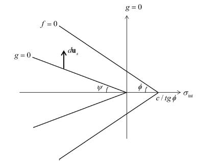
In order to define the interval of stress states that correspond to reversible relative displacements, a yield criterion must be defined. In the present work, the Mohr-Coulomb yield criterion is adopted (see Fig. 2):

$\text{f}=\left|{\tau }_{\mathrm{int}}\right|+\mu {\sigma }_{\mathrm{int}}-c$ (18)

where c is the cohesion and μ is the friction coefficient of the material interface. Coefficient μ is usually defined from the internal friction angle ϕ: $\mu =tg\varphi$ . The stress vector acting upon a current point of the interface is defined in terms of the tangential (τ_int) and normal (σ_int) stress components. The tangential stress component is updated according to the elastic-plastic formulation, where the yield criterion described above indicates if the stress increment associated with the relative displacement on the interface is obtained using an elastic constitutive equation or an elastic-plastic constitutive equation.

We deal now with the crucial issue related to how the normal vector $v$ to cylindrical interface can be defined in the plane of inclusion cross-section (see Fig. 3). It is emphasized that this key point is inherent to the mixed 3D-1D formulation when the interface behavior is accounted for. The underlying question is: how interaction forces between a 1D structural element and the surrounding 3D continuous body are possibly modeled from a rigorous mechanical viewpoint? An approximate approach to deal with this challenging issue has been proposed in Figueiredo et al. (2013). In the subsequent analysis, we develop a heuristic approach in which interaction efforts are defined from minimization of the shear component of the stress vector generated on all the facets of the soil/inclusion interface by the stress tensor in the soil. The stress vector acting along the interface is first computed from the stress tensor σ _m in the solid matrix:

$t={\sigma }_{\text{m}}.v$ (19)

The normal stress is simply the projection of $t$on the normal direction:

${\sigma }_{\mathrm{int}}=t.v$ (20)

From a computational viewpoint, tensor σm is evaluated at macroscopic points of the matrix element containing the inclusion element, coinciding with the integration points of the inclusion element. Unit normal vector v is defined in the global coordinate system (X1, X2, X3) by its orientation θ in the inclusion cross-section plane and the direction cosines li, mi and ni of the local frame (l, m, n):

$v=\left[\begin{array}{ccc}{l}_1& l_2& l_3\\ m_1& m_2& m_3\\ n_1& n_2& n_3\end{array}\right].\left\{\begin{array}{c}0\\ \cos \theta \\ \sin \theta \end{array}\right\}$ (21)

Figure 3
Stress vector acting at matrix/inclusion interface and corresponding normal component.

The inclusion is geometrically described by a curvilinear structure in the 3D-1D mixed formulation, where the orientation $\theta$ of the normal vector v is arbitrary. To resolve this indetermination, the subsequent analysis considers the orientation $\theta$ that minimizes the value of shear stress $c-\mu {\sigma }_{\mathrm{int}}$ complying with the yield criterion (18). This arbitrary definition implicitly assumes a constant stress state when moving around the soil/inclusion interface, which could reveal questionable in some situations. It is readily shown that condition dσ_int/dθ = 0 yields:

$tg2\theta =\frac{{\rm B}}{{\rm A}-\text{C}}$ (22)

with:

${\rm A}={\sigma }_{11\text{m}}{l}_2^2+{\sigma }_{22\text{m}}{m}_2^2+{\sigma }_{33\text{m}}{n}_2^2+2{\sigma }_{12\text{m}}{l}_2{m}_2+2{\sigma }_{13\text{m}}{l}_2{n}_2+2{\sigma }_{23\text{m}}{m}_2{n}_2$ (23)

$\begin{array}{l}B=2{\sigma }_{11\text{m}}{l}_2{l}_3+2{\sigma }_{22\text{m}}{m}_2{m}_3+2{\sigma }_{33\text{m}}{n}_2{n}_3+\\ 2{\sigma }_{12\text{m}}\left(l_2{m}_3+l_3{m}_2\right)+2{\sigma }_{13\text{m}}\left(l_2{n}_3+l_3{n}_2\right)+2{\sigma }_{23\text{m}}\left(m_2{n}_3+m_3{n}_2\right)\end{array}$ (24)

$C={\sigma }_{11\text{m}}{l}_3^2+{\sigma }_{22\text{m}}{m}_3^2+{\sigma }_{33\text{m}}{n}_3^2+2{\sigma }_{12\text{m}}{l}_3{m}_3+2{\sigma }_{13\text{m}}{l}_3{n}_3+2{\sigma }_{23\text{m}}{m}_3{n}_3$ (25)

The solution to Equation (22) that leads to higher value of ${\sigma }_{\mathrm{int}}$ is hence retained.

The direction of relative plastic displacement is derived from the flow rule given as follows:

$d{u}_s^{ir}=d{\lambda }^{\prime }\frac{\partial g}{\partial {\tau }_{\mathrm{int}}}$ (26)

$d{u}_n^{ir}=d{\lambda }^{\prime }\frac{\partial g}{\partial {\sigma }_{\mathrm{int}}}$ (27)

where $d{\lambda }^{\prime }$ is the plastic multiplier and g is the plastic potential. The latter is assumed under form:

$\text{g}=\left|{\tau }_{\mathrm{int}}\right|+\text{tg}\psi {\sigma }_{\mathrm{int}}$ (28)

where $\psi \le \varphi$ is the dilatancy angle.

The consistency condition employed in the present formulation may be expressed as:

$\frac{\partial \text{f}}{\partial {\tau }_{\mathrm{int}}}d{\tau }_{\mathrm{int}}+\frac{\partial \text{f}}{\partial {\sigma }_{\mathrm{int}}}d{\sigma }_{\mathrm{int}}+\frac{\partial \text{f}}{\partial \text{c}}d\text{c}=0$ (29)

The last term of the equation above is related to material hardening when this feature is considered in the mechanical description of the material. A linear isotropic strain hardening model is assumed here to describe the cohesion evolution after yielding, which may be expressed as follows:

$d\text{c}=hd{u}_s^{ir}$ (30)

where h is the hardening modulus. Notice that the cohesion evolution does not explicitly depend on the normal component of the stress state along the interface.

Recalling that the normal component of the total relative displacement $d{u}_n^{}$ is zero, one obtains:

$d{u}_n^{el}+d{u}_n^{ir}=0\Rightarrow d{u}_n^{el}=-d{\lambda }^{\prime }\frac{\partial g}{\partial {\sigma }_{\mathrm{int}}}$ (31)

The elastic constitutive equation describing the behavior of interface written in terms of differential stress components and differential relative displacements reads:

$\{\begin{array}{l}d{\sigma }_{\mathrm{int}}=k_{n}d{u}_n^{el}\\ d{\tau }_{\mathrm{int}}=k_s\text{}d{u}_s^{el}\end{array}$ (32)

in which k_n and k_s refer to normal and tangential stiffness moduli. It is observed that these quantities are expressed in units of force per cubic length [Pa/m].

By substituting Eq. (31) into the constitutive equation corresponding to the normal stress component, the plastic multiplier can be obtained as follows:

$d{\lambda }^{\prime }=-\frac{d{\sigma }_{\mathrm{int}}}{k_n\text{tg}\psi }$ (33)

On the other hand, making use of the consistency equation together with constitutive equations (32) leads to:

$d{\sigma }_{\mathrm{int}}=sign(\tau )\frac{hd\lambda ´-d{\tau }_{\mathrm{int}}}{tg\varphi }$ (34)

Finally, the plastic multiplier may be rewritten as follows:

$d{\lambda }^{\prime }=\frac{sign({\tau }_{\mathrm{int}})}{k_n\text{}tg\varphi tg\psi +hsign({\tau }_{\mathrm{int}})}d{\tau }_{\mathrm{int}}$ (35)

It stems from the constitutive equation of the interface following the tangential direction that:

$d{\tau }_{\mathrm{int}}=k_s\left(d{u}_s-d{u}_s^{ir}\right)=k_s\left(d{u}_s-d{\lambda }^{\prime }\frac{\partial g}{\partial {\tau }_{\mathrm{int}}}\right)$ (36)

Taking into account the particular form (28) of potential $g$ and expression (35) of plastic multiplier, the elastoplastic constitutive equation of the matrix-reinforcement interface is given as follows:

$d{\tau }_{\mathrm{int}}=\frac{k_s}{1+\frac{k_s}{k_n\text{}tg\varphi tg\psi +hsign({\tau }_{\mathrm{int}})}}d{u}_s$ (37)

Therefore, the incremental form of the constitutive equations referring to the contact interface reads:

$\Delta {\tau }_{\mathrm{int}}=k_s\Delta u_s$ (38)

in the elastic range, and:

$\Delta {\tau }_{\mathrm{int}}=\frac{k_s}{1+\frac{k_s}{k_n\text{}tg\varphi tg\psi +hsign({\tau }_{\mathrm{int}})}}\Delta u_s$ (39)

in the plastic range. When $\psi \to 0$ (no dilation), condition $d{u}_n^{}=0$ can be ensured by choosing $k_n\text{}/k_s~1/tg\psi$.

3 FINITE STRAIN APPROACH

Nonlinear problems are usually analyzed employing the incremental approach, where strain increments are evaluated based on the last incremental displacement field obtained from the solution of the equilibrium equations. At each iterative step, the respective stress updates are obtained according to the material behavior. When large strains are involved, the latter can be described in the corotational coordinate system adopting objective stress rate.

Although the matrix and the inclusions may undergo large strains, a fundamental assumption of the present modeling is that the strains along matrix/inclusions interface remain infinitesimal.

3.1 Corotational description of matrix particles motion

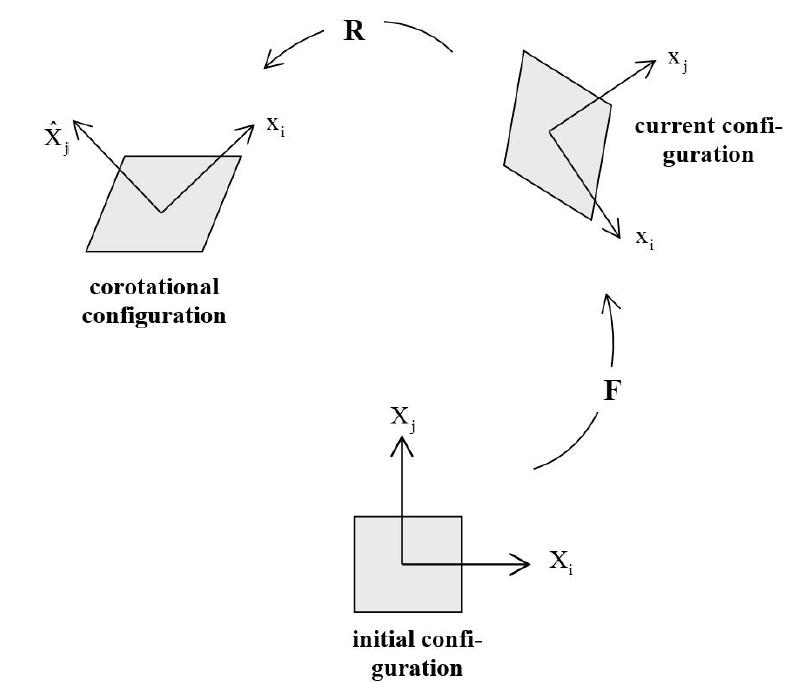
A basic issue to the corotational description of the motion of a continuum body is the decomposition of the reference frame into base and corotated configurations (Felippa and Haugen, 2005a, 2005b). The base configuration usually refers to the undeformed configuration, while the corotated one is obtained through a rigid body motion from the base configuration. The coordinate system of the corotated configuration follows the material motion and can be easily related to the global coordinate system through rotation operations. In the finite element approach, each element possesses its own set of coordinate systems located at the respective quadrature points.

Figure 4
Quadrature-attached frame.

The starting point of the analysis is the decomposition of geometric transformation of matrix into a rigid body motion and pure deformation performed at the element level in the corotational coordinate system. Such a corotational description maintains orthogonality of the attached reference frame as illustrated in Figure 4, thus providing an effective setting for rate form formulation of the constitutive equations in the context of large strains. Note that rotation $R$ transforming the current configuration into corotational configuration can be defined from the rotation component in polar decomposition of deformation gradient (Espath et al., 2014).

Assuming that all kinematical variables are known at the previous configuration t = t _n of the matrix, the displacement field at the end of the current load step can be obtained from integration of the strain rate tensor along time interval [t _n, t _n+1]. The whole steps of the reasoning are performed in the corotational coordinate system, where notation $\widehat{\mathcal{Q}}$ shall be used to express any field $\mathcal{Q}$ in the corotational frame. The strain rate tensor in the corotational system is defined as:

${\widehat{d}}_{\text{m}}=\frac{1}{2}\left[\frac{\partial {\widehat{v}}_m^{def}}{\partial {\widehat{x}}_{}}+{\left(\frac{\partial {\widehat{v}}_m^{def}}{\partial {\widehat{x}}_{}}\right)}^T\right]$ (40)

where ${\widehat{v}}_m^{def}$ represents the velocity field associated with the deformation part of the motion expressed in the corotational system. The strain increment is computed using the mid-point integration proposed in Hughes and Winget (1980). In this procedure the velocity is assumed to be constant within the time interval and the reference configuration is attached to the intermediate configuration at t = t _n+1/2 in the corotational system. Accordingly:

${\displaystyle \underset{t_n}{\overset{t_{n+1}}{\int }}{\widehat{d}}_{\text{m}}d\tau }\cong \frac{1}{2}\left[\frac{\partial \Delta {\widehat{u}}_m^{def}}{\partial {\widehat{x}}_{n+1/2}}+{\left(\frac{\partial \Delta {\widehat{u}}_m^{def}}{\partial {\widehat{x}}_{n+1/2}}\right)}^T\right]=\Delta {\widehat{\epsilon }}_{\text{m}}$ (41)

where $\Delta {\widehat{u}}_m^{def}$ is referred to the deformation part of the total displacement increment $\Delta {\widehat{u}}_{\text{m}}$ in the corotational system and ${\widehat{x}}_{n+1/2}$ is the intermediate geometric configuration of the matrix element in the corotational system, which can be computed as:

${\widehat{x}}_{n+1/2}=R_{n+1/2}\cdot x_{n+1/2}=\frac{1}{2}{R}_{n+1/2}\cdot \left(x_n+x_{n+1}\right)$ (42)

where $R_{n+1/2}$ is the orthogonal transformation tensor performing rotation from the global coordinate system to the corotational coordinate system defined locally at the intermediate configuration $t_{n+1/2}$ of the matrix element. The displacement increment $\Delta u_{\text{m}}$ referring to time interval [t _n, t _n+1] is decomposed at element level according to:

$\Delta u_{\text{m}}=\Delta u_m^{def}+\Delta u_m^{rot}$ (43)

In the above local relationship, $\Delta u_m^{def}$ and $\Delta u_m^{rot}$ denote respectively the deformation and rotation parts of the displacement increment defined in the global coordinate system.

The increment of deformation displacements expressed in the corotational system is defined by:

$\Delta {\widehat{u}}_m^{def}={\widehat{x}}_{n+1}-{\widehat{x}}_n=R_{n+1/2}\cdot \Delta u_m^{def}$ (44)

since the strain rate tensor is evaluated at the intermediate configuration $t_{n+1/2}$. Coordinates ${\widehat{x}}_n$ and ${\widehat{x}}_{n+1}$corresponding to geometric configurations in the corotational system at $t=t_n$ and $t=t_{n+1}$ are obtained from the following transformations:

${\widehat{x}}_n=R_n\cdot x_n\text{and}{\widehat{x}}_{n+1}=R_{n+1}\cdot x_{n+1}$ (45)

where $R_n$ and $R_{n+1}$are orthogonal transformation tensors performing rotations from the global coordinate system to the corotational coordinate system defined locally at $t=t_n$ and $t=t_{n+1}$, respectively. Vectors $x_n$ and $x_{n+1}$ refer to geometric configurations defined in the global coordinate system. Omitting subscripts $\left\{n,n+1/\mathrm{2,}n+1\right\}$ referring to considered time, the components of the transformation $R$are given by:

$R_{1j}=\frac{r_{1j}}{r_1^T{r}_1};R_{2j}=\frac{(r_{2j}+r_{cj})}{{(r_{2j}+r_{cj})}^T(r_{2j}+r_{cj})};R_{3j}=\frac{r_{3j}}{r_3^T{r}_3}(j=\mathrm{1,2,3})$ (46)

with:

$r_{1j}={\xi }^T{x}_j;r_{2j}={\eta }^T{x}_j;r_{cj}=-\frac{r_{1j}^T{r}_{2j}}{r_{1j}^T{r}_{1j}}{r}_{1j};r_{3j}=r_{1j}\times (r_{2j}+r_{cj})$ (47)

$\left(\xi ,\eta ,\zeta \right)$ and $x$ are vectors containing local nodal coordinates and global nodal coordinates associated with the considered finite element, respectively (Duarte Filho and Awruch, 2004).

The Cauchy stress tensor in the global system is obtained from objective tensor transformation as follows:

${\sigma }_{\text{m}}=R^T{\widehat{\sigma }}_{\text{m}}R$ (48)

where ${\sigma }_{\text{m}}$ and ${\widehat{\sigma }}_{\text{m}}$ are the Cauchy stress tensors evaluated in the global and corotational system, respectively. To formulate the constitutive behavior of matrix constitutive material, a set of assumptions are stated. First, the elastic part of the deformation gradient of matrix particles is assumed to remain infinitesimal, meaning that large strains are of irreversible (plastic) nature. In addition, the constitutive material is considered as elastically isotropic and that elastic properties are not affected by the plastic strains. Under these conditions, it can be shown that the state equation formulated in rate form relates a rotational time derivative of stress tensor (Jaumman derivative) and the strain rate tensor (see for instance Dormieux and Maghous, 1999; Bernaud et al., 2002; Bernaud et al., 2006) through:

${\dot{\widehat{\sigma }}}_{\text{m}}^J={\widehat{D}}^e\cdot \left({\widehat{d}}_{\text{m}}-{\widehat{d}}_{\text{m}}^{\text{p}}\right)with{\dot{\widehat{\sigma }}}_{\text{m}}^J={\dot{\widehat{\sigma }}}_{\text{m}}+{\widehat{\sigma }}_{\text{m}}\cdot {\widehat{\Omega }}_{\text{m}}-{\widehat{\Omega }}_{\text{m}}\cdot {\widehat{\sigma }}_{\text{m}}$ (49)

where ${\widehat{d}}_{\text{m}}^{\text{p}}$ denotes the plastic strain rate and ${\widehat{\Omega }}_{\text{m}}$is the spin tensor defined in the corotational system. The above equation is used for stress updates in the corotational system in the context of large strains. It is observed that the corotational spin tensor has also to be integrated over the time interval $[t_n,t_{n+1}]$ following the same mid-point rule adopted in (41).

3.2 Description of deformation in embedded inclusion

As adopted for surrounding matrix, the kinematics of the embedded inclusion is described referring to configuration $t_n$. With respect to this configuration, the Green-Lagrange axial strain writes:

$E_{\text{c}}=\frac{\partial u_c}{\partial x_t}+\frac{1}{2}{\left[\frac{\partial u_c}{\partial x_t}\right]}^{{\rm T}}\left[\frac{\partial u_c}{\partial x_t}\right]\text{with}{u}_c=u_{\text{c}}\cdot l$ (50)

where $u_{\text{c}}$ is the displacement vector at any point along the embedded inclusion. Derivations are taken with respect to coordinate $x_t=x_l$ along the tangential direction, as illustrated in Figure 5.

It is recalled that the displacement jump at the surrounding matrix/inclusion interface is purely tangential (see section 2.1):

$u_{\text{c}}-u_m=u_{s}l$ (51)

where $l$ is the unit vector along the cable. Accordingly, the components of $u_{\text{c}}$ in the local coordinate system may be expressed from $u_s$and the displacement components in the global coordinate system umT = (um,1, um,2, um,3) of the geometrically coinciding matrix particle:

$u_c=u_{s}l+R^{\ast }.u_m=\left\{\begin{array}{c}{u}_s\\ 0\\ 0\end{array}\right\}+\left[\begin{array}{ccc}{l}_1& l_2& l_3\\ m_1& m_2& m_3\\ n_1& n_2& n_3\end{array}\right].\left\{\begin{array}{c}{u}_{\text{m}\text{,1}}\\ u_{\text{m}\text{,2}}\\ u_{\text{m}\text{,3}}\end{array}\right\}$ (52)

Figure 5
Displacements of an element of embedded inclusion.

As defined in Figure 1, li, mi and ni are the direction cosines of inclusion local axes $(l,m,n)$ with respect to the global coordinate system$(X_1,X_2,X_3)$. Matrix $R^{\ast }$ is the coordinate rotation transformation between local and global frames.

The axial strain $E_{\text{c}}$ is computed using the matrix notation (52):

$\frac{\partial u_c}{\partial x_t}\equiv \left\{\begin{array}{c}\partial u_c/\partial x_t\\ \partial v_c/\partial x_t\\ \partial w_c/\partial x_t\end{array}\right\}=\left\{\begin{array}{c}\partial u_s/\partial x_t\\ 0\\ 0\end{array}\right\}+R^{\ast }.\left[\begin{array}{ccc}\partial u_m/\partial x& \partial u_m/\partial y& \partial u_m/\partial z\\ \partial v_m/\partial x& \partial v_m/\partial y& \partial v_m/\partial z\\ \partial w_m/\partial x& \partial w_m/\partial y& \partial w_m/\partial z\end{array}\right]\left\{\begin{array}{c}{l}_1\\ l_2\\ l_3\end{array}\right\}$ (53)

The embedded curvilinear inclusion is discretized by means of succession of linear elements. Each element is embedded within a brick element (parent element) associated with a constant tangent vector $l$ and a constant matrix transfer R*. When perfect bonding is considered at the interface solid matrix/inclusion, the first term in the right hand-side of (53) should be removed (i.e., $\partial u_s/\partial x_t=0$).

Keeping in mind that the approach is based on the updated Lagrangian scheme, the axial strain $E_{\text{c}}$ is defined referring to the last equilibrated configuration of the embedded inclusion. The latter configuration is defined in the corotational coordinate system referring to the embedding matrix element (parent element) as sketched in Figure 6.

Figure 6
Updated Lagrangian scheme and corotational configuration in the context of embedded approach.

Assuming an elastic behavior for the inclusion constitutive material, the stress increment during time interval $[t_n,t_{n+1}]$ is related to axial strain by means of the uniaxial linear relationship:

$\Delta \pi =E_c{E}_{\text{c}}$ (54)

$\pi$ is the second Piola-Kirchhoff stress tensor and $E_c$ is the elastic stiffness of the inclusion constitutive material.

3.3 Finite element discretization

In the subsequent analysis the eight-node hexahedral finite element formulation with one-point quadrature is adopted to discretize the displacements of matrix particles. At the element level, the displacement vector of matrix particles between $t_n$ and $t_{n+1}$ is approximated, using Voigt notation, as follows:

$u_m=x_m^{t_{n+1}}-x_m^{t_n}=N_m{u}_m^{\ast }\text{with}{N}_m=\left[\begin{array}{ccc}N& 0& 0\\ 0& N& 0\\ 0& 0& N\end{array}\right]$ (55)

where $u_m^{\ast }$ is the vector of nodal displacements referring to eight-node hexahedral element and $N_m$is the $3\times 24$ matrix defined by sub-matrix $N=\left[{\text{N}}_1,\dots ,{\text{N}}_8\right]$ that contains the associated shape functions. In the context of geometrically nonlinear analysis, these quantities are evaluated considering the current configuration of the element in the corotational coordinate system (${\widehat{u}}_m^{\ast }$and ${\widehat{N}}_m$, respectively). At element level, the strain increment is thus computed according to:

$\Delta {\epsilon }_m=B_m{u}_m^{\ast }$ (56)

$B_m$ being the $3\times 24$ matrix aimed to generate the symmetric part of the displacement gradient at element level (see Eq. (41)). It is should be observed that matrix $B_m$ must be also evaluated considering the differential operator in the corotational coordinate system, that is operating with ${\widehat{B}}_m$. Finally, similar procedures are used for the finite element approximation of strain rate tensor and spin tensor.

Regarding the embedded inclusions, their geometry is discretized into piecewise linear elements. Instead of nodal displacements of the inclusion elements, the approach operates with nodal displacements jump. Along each two-node element, the tangential relative displacement between matrix and inclusion particles defined in (4) is approximated from the nodal values:

$u_s=\Phi u_s^{\ast }$ (57)

where $u_s^{\ast }$ is the tangential displacement jump vector related to the linear finite element nodes of the embedded inclusion. Matrix Φ, whose dimension is $1\times 2$, contains the shape functions of the two-node linear element.

Recalling that $u_c=u_{s}l+R^{\ast }.u_m$ (see equations (51) and (52)), the discretized expression of axial Green-Lagrange strain between $t_n$ and $t_{n+1}$ reads in each inclusion element:

$E_{\text{c}}={{\rm B}}_{\text{s}}{u}_s^{\ast }+{{\rm T}}_{\epsilon }{{\rm B}}_m{u}_m^{\ast }+\frac{1}{2}{d}^{\ast T}{G}^{T}G\text{}{d}^{\ast }$ (58)

where $B_s=\frac{d\Phi }{d{x}_t}$ is the $1\times 2$matrix containing the derivatives of shape functions with respect to tangential coordinate along the inclusion element, $T_{\epsilon }$is the $1\times 6$matrix introduced in (2). Matrix $G\text{}$, whose dimensions are $3\times 26$, is defined by:

$G=\left[\begin{array}{cccc}\frac{\partial N}{\partial x_j}{l}_1{l}_j& \frac{\partial N}{\partial x_j}{l}_2{l}_j& \frac{\partial N}{\partial x_j}{l}_3{l}_j& \frac{\partial \Phi }{\partial x_t}\\ \frac{\partial N}{\partial x_j}{m}_1{l}_j& \frac{\partial N}{\partial x_j}{m}_2{l}_j& \frac{\partial N}{\partial x_j}{m}_3{l}_j& 0\\ \frac{\partial N}{\partial x_j}{n}_1{l}_j& \frac{\partial N}{\partial x_j}{n}_2{l}_j& \frac{\partial N}{\partial x_j}{n}_3{l}_j& 0\end{array}\right]$ (59)

Vector $d^{\ast }$contains 26 components of nodal displacements associated with the matrix element (brick element) and embedded linear inclusion element:

$d^{\ast }=\left\{\begin{array}{c}{u}_m^{\ast }\\ u_s^{\ast }\end{array}\right\}$ (60)

Rearranging (58) yields:

$E_{\text{c}}=\left[\begin{array}{cc}{{\rm T}}_{\epsilon }{{\rm B}}_m& {{\rm B}}_{\text{s}}\end{array}\right]\text{}{d}^{\ast }+\frac{1}{2}{d}^{\ast T}{G}^{T}G\text{}{d}^{\ast }$ (61)

It is observed that $\left[\begin{array}{cc}{{\rm T}}_{\epsilon }{{\rm B}}_m& {{\rm B}}_{\text{s}}\end{array}\right]$is a $1\times 26$matrix defined from sub-matrices ${{\rm T}}_{\epsilon }{{\rm B}}_m$ and ${{\rm B}}_{\text{s}}$.

If perfect bonding is considered at the matrix/inclusion interface, the latter expression reduces to

$E_{\text{c}}={{\rm T}}_{\epsilon }{{\rm B}}_m{u}_m^{\ast }+\frac{1}{2}{u}_m^{\ast T}{\tilde{G}}^T\tilde{G}\text{}{u}_m^{\ast }$ (62)

where matrix $\tilde{G}\text{}$ is obtained from matrix $G$ by removing its last two columns.

The subsequent developments deal with the finite element formulation of the equations governing the response of the mechanical system to a prescribed external loading. It is recalled that the mechanical system refers to the solid matrix and embedded inclusions in mutual interaction. Discretization of the weak form of balance momentum expressed at current configuration of the mechanical system results in a set of nonlinear equations. These equilibrium equations must be iteratively satisfied using the incremental approach (see Bathe, 1996), since both the stiffness matrices and the internal force vectors are functions of the current element configuration. A linearization procedure based on Newton-Raphson method and Taylor series expansion of the general internal force vector within the time interval $[t_n,t_{n+1}]$ leads to the following global system:

$K_{n+\mathrm{1,}i-1}^{\tan }(U)U_{n+1,i}=F_{n+1}^{ext}-F_{n+\mathrm{1,}i-1}^{\mathrm{int}}(U)$ (63)

where subscript $n+1$ denotes the current position in the time marching, while subscripts $i$ and $i-1$ refer respectively to current and previous iterative steps in the Newton-Raphson procedure applied over the time interval $[t_n,t_{n+1}]$. $K_{}^{\tan }$ is the tangent stiffness matrix, $F_{}^{ext}$ and $F_{}^{\mathrm{int}}$ are the external and internal force vectors, respectively. $U$ represents the global vector whose components are node values of the matrix displacement and the interface relative displacement between $t_n$ and $t_{n+1}$. Vector $U$ is obtained by assembling procedure to incorporate the contribution of all element nodal displacements $u_m^{\ast }$ or $d^{\ast }$.

At each iterative step, the stiffness matrix and the internal force vector are evaluated in the corotational coordinate system. In particular, the terms related to the elementary contribution of matrix (matrix element without embedded inclusion) take the following expressions:

${\widehat{k}}_m^{tan}={\displaystyle \underset{{\widehat{\Omega }}_m^e}{\int }{\widehat{B}}_m^T\left({\widehat{D}}^{ep}+{\widehat{D}}^{geo}\right)}{\widehat{B}}_{m}d{\widehat{\Omega }}_m^e;{\widehat{f}}_m^{\mathrm{int}}={\displaystyle \underset{{\widehat{\Omega }}_m^e}{\int }{\widehat{B}}_m^T}{\widehat{\sigma }}_{\text{m}}d{\widehat{\Omega }}_m^e$ (64)

where ${\widehat{\Omega }}_m^e$ stands for the current configuration of the matrix element volume in the corotational system. ${\widehat{D}}^{ep}$ is the stress-strain constitutive matrix defined in (49), ${\widehat{D}}^{geo}$ is the geometric stiffness matrix associated with the Jaumann rate terms ${\widehat{\sigma }}_{\text{m}}\cdot {\widehat{\Omega }}_{\text{m}}-{\widehat{\Omega }}_{\text{m}}\cdot {\widehat{\sigma }}_{\text{m}}$, and ${\widehat{\sigma }}_{\text{m}}$ is the corotational Cauchy stress tensor (see Braun and Awruch, 2008; Duarte Filho and Awruch, 2004 for further details). In order to solve the equilibrium equation, the tangent stiffness matrix and the internal force vector are brought back to the global coordinate system using the following objective transformations:

$k_m^{tan}=R^T{\widehat{k}}_m^{tan}R;f_m^{int}=R^T{\widehat{f}}_m^{int}$ (65)

where $R$ is the rotation transformation matrix defined in Eqs. (45) and (46).

The finite element formulation is based on reduced integration, where hourglass control techniques are employed in order to avoid numerical instabilities, such as volumetric locking and/or shear locking. Detailed description of the stabilization procedures adopted in this work may be found in Braun and Awruch (2008, 2013).

As regards the contribution of embedded inclusions to tangent stiffness matrix and force vector, the work performed by the internal axial force $\pi$ in any virtual elastic evolution $\delta E_{\text{c}}$ should be analyzed. Denoting by ${\widehat{\Omega }}_c^e$ the last equilibrated configuration of the inclusion element with respect to the corotational system of the surrounding matrix element (parent element), the internal force vector related to inclusion element is defined as:

${\widehat{f}}_c^{\mathrm{int}}={\displaystyle \underset{{\widehat{\Omega }}_c^e}{\int }{\left[\begin{array}{cc}{{\rm T}}_{\epsilon }.{\widehat{{\rm B}}}_m& {\widehat{{\rm B}}}_{\text{s}}\end{array}\right]}^T\pi d{\widehat{\Omega }}_c^e}+{\displaystyle \underset{{\widehat{\Omega }}_c^e}{\int }{\widehat{G}}^T\widehat{G}{d}^{\ast }{\pi }_{}d{\widehat{\Omega }}_c^e}$ (66)

The elementary tangent stiffness matrix due to inclusion contribution is obtained by linearizing the above expression of internal force vector with respect to generalized displacement vector $d={\left[u_m^{},u_s^{}\right]}^{\text{}\text{T}}$ (see Eq. (60)):

${\widehat{k}}_c^{tan}={\displaystyle \underset{{\widehat{\Omega }}_c^e}{\int }{\left[\begin{array}{cc}{{\rm T}}_{\epsilon }.{\widehat{{\rm B}}}_m& {\widehat{{\rm B}}}_{\text{s}}\end{array}\right]}^T{E}_c}\left[\begin{array}{cc}{{\rm T}}_{\epsilon }.{\widehat{{\rm B}}}_m& {\widehat{{\rm B}}}_{\text{s}}\end{array}\right]d{\widehat{\Omega }}_c^e+{\displaystyle \underset{{\widehat{\Omega }}_c^e}{\int }{\widehat{G}}^T\widehat{G}{\sigma }_{c}d{\widehat{\Omega }}_c^e}$ (67)

where $E_c$is the longitudinal elastic stiffness of inclusion material and ${\sigma }_c$ is the axial Cauchy stress tensor along the inclusion element.

For a single element with embedded inclusion segment, the discretized weak form of equilibrium equation writes

${\left(\left[\begin{array}{cc}{k}_{mm}+k_{mm,cc}& k_{mc}\\ k_{cm}& k_{cc}+k_{ss}\end{array}\right]+\left[k_G\right]\right)}_{n+\mathrm{1,}i-1}{\left\{\begin{array}{c}{u}_m^{\ast }\\ u_s^{\ast }\end{array}\right\}}_{n+\mathrm{1,}i}={\left\{\begin{array}{c}{f}_m^{ext}+f_{m,c}^{ext}\\ f_s^{ext}\end{array}\right\}}_{n+1}-{\left\{\begin{array}{c}{f}_m^{int}+f_{m,c}^{int}\\ f_s^{int}+f_{s,c}^{int}\end{array}\right\}}_{n+\mathrm{1,}i-1}$ (68)

where:

$k_{mm}=R^T{\widehat{k}}_{mm}R\text{with}{\widehat{k}}_{mm}={\displaystyle \underset{{\widehat{\Omega }}_m^e}{\int }{\widehat{B}}_m^T\left({\widehat{D}}^{ep}+{\widehat{D}}^{geo}\right)}{\widehat{B}}_{m}d{\widehat{\Omega }}_m^e$ (69)

$k_{mm,cc}=R^T{\widehat{k}}_{mm,cc}R\text{with}{\widehat{k}}_{mm,cc}={\displaystyle \underset{{\widehat{L}}_c^e}{\int }{\left[{{\rm T}}_{\epsilon }{\widehat{{\rm B}}}_m\right]}^T{E}_c{A}_c}\left[{{\rm T}}_{\epsilon }{\widehat{{\rm B}}}_m\right]d{\widehat{L}}_c^e$ (70)

$k_{cc}=R^T{\widehat{k}}_{cc}R\text{with}{\widehat{k}}_{cc}={\displaystyle \underset{{\widehat{L}}_c^e}{\int }{\widehat{{\rm B}}}_{\text{s}}{}^T{E}_c}{A}_c{\widehat{{\rm B}}}_{\text{s}}d{\widehat{L}}_c^e$ (71)

$k_{mc}=R^T{\widehat{k}}_{mc}R\text{with}{\widehat{k}}_{mc}={\displaystyle \underset{{\widehat{L}}_c^e}{\int }{\left[{{\rm T}}_{\epsilon }.{\widehat{{\rm B}}}_m\right]}^T{E}_c{A}_c}{\widehat{{\rm B}}}_{\text{s}}d{\widehat{L}}_c^e$ (72)

$k_{cm}=R^T{\widehat{k}}_{cm}R\text{with}{\widehat{k}}_{cm}={\displaystyle \underset{{\widehat{L}}_c^e}{\int }{\widehat{{\rm B}}}_{\text{s}}{}^T{E}_c{A}_c}\left[{{\rm T}}_{\epsilon }{\widehat{{\rm B}}}_m\right]d{\widehat{L}}_c^e$ (73)

$k_{ss}=R^T{\widehat{k}}_{ss}R\text{with}{\widehat{k}}_{ss}={\displaystyle \underset{{\widehat{L}}_c^e}{\int }{\Phi }^{{\rm T}}{K}_{\text{b},\text{t}}\Phi {\text{P}}_{\text{c}}d{\widehat{L}}_c^e}$ (74)

$k_G={\displaystyle \underset{{\widehat{\Omega }}_c^e}{\int }{\widehat{G}}^T\widehat{G}{\sigma }_{c}d{\widehat{\Omega }}_c^e}$ (75)

$f_m^{int}=R^T{\widehat{f}}_m^{int}\text{with}{\widehat{f}}_m^{int}={\displaystyle \underset{{\widehat{\Omega }}_m^e}{\int }{\widehat{B}}_m^T{\widehat{\sigma }}_{m}d{\widehat{\Omega }}_m^e}$ (76)

$f_{m,c}^{int}=R^T{\widehat{f}}_{m,c}^{int}\text{with}{\widehat{f}}_{m,c}^{int}={\displaystyle \underset{{\widehat{L}}_c^e}{\int }{\left[{{\rm T}}_{\epsilon }.{\widehat{{\rm B}}}_m\right]}^T{\sigma }_c{\text{A}}_{\text{c}}d{\widehat{L}}_c^e}$ (77)

$f_s^{int}=R^T{\widehat{f}}_s^{int}\text{with}{\widehat{f}}_s^{int}={\displaystyle \underset{{\widehat{L}}_c^e}{\int }{\Phi }^{{\rm T}}{\tau }_{\mathrm{int}}{P}_{\text{c}}\text{d}{\widehat{L}}_c^e}$ (78)

$f_{s,c}^{int}=R^T{\widehat{f}}_{s,c}^{int}\text{with}{\widehat{f}}_{s,c}^{int}={\displaystyle \underset{{\widehat{L}}_c^e}{\int }{\widehat{{\rm B}}}_{\text{s}}{}^T{\sigma }_c{\text{A}}_{\text{c}}\text{d}{\widehat{L}}_c^e}$ (79)

$f_m^{ext}={\displaystyle \underset{{\widehat{\Omega }}_m^e\cap {\Gamma }_m}{\int }{N}_m^T{\overline{t}}_m\text{d}{\Gamma }_m}+{\displaystyle \underset{{\widehat{\Omega }}_m^e}{\int }{N}_m^T{b}_m\text{d}{\widehat{\Omega }}_m^e}$ (80)

$f_{m,c}^{ext}={\displaystyle \underset{{\widehat{\Omega }}_c^e\cap {\Gamma }_c}{\int }{N}_m^T{\overline{t}}_c\text{d}{\Gamma }_c}+{\displaystyle \underset{{\widehat{L}}_c^e}{\int }{N}_m^T{b}_c{\text{A}}_{\text{c}}\text{d}{\widehat{L}}_c^e}$ (81)

$f_s^{ext}={\displaystyle \underset{{\widehat{\Omega }}_c^e\cap {\Gamma }_c}{\int }{\Phi }_{}^T\left({\overline{t}}_c\cdot l\right)\text{d}{\Gamma }_c}+{\displaystyle \underset{{\widehat{L}}_c^e{}_c}{\int }{\Phi }_{}^T\left(b_c\cdot l\right)}{\text{A}}_{\text{c}}\text{d}{\widehat{L}}_c^e$ (82)

For a matrix element without embedded inclusion, (68) reduces to:

${\left[k_{mm}\right]}^{n+\mathrm{1,}i-1}{\left\{u_m^{\ast }\right\}}^{n+\mathrm{1,}i}={\left\{f_m^{ext}\right\}}^{n+1}-{\left\{f_m^{int}\right\}}^{n+\mathrm{1,}i-1}$ (83)

After assembling all the elements, the global system takes the form given by Eq. (63), which is solved iteratively with implementation of Generalized Displacement Control Method (e.g. Yang and Shieh, 1990).

4 VERIFICATION TEST OF NUMERICAL PROCEDURE

In order to check the finite element implementation of the proposed model as well as related accuracy, the numerical simulation of a kind of inclusion pull-out test is analyzed in the sequel. The structure sketched in Fig. 7 consists of a reinforced cantilever beam with length L and rectangular b x h cross-section. The loading is defined by the following conditions:

• body forces are neglected;

• both matrix and inclusion are clamped along the plane x = 0;

• a force $P{\underset{\_}{e}}_x$ is applied at the free end of the reinforcing inclusion, while the matrix is free of stresses along the plane x = L.

The matrix constituent material is elastic perfectly plastic with a von Mises condition for plastic yielding. A Mohr-Coulomb elastoplastic constitutive law with a non associated plastic flow is considered for the matrix/inclusion interface. The corresponding model data are given in Table 1. The finite element grid used for the simulation is shown in Fig. 7 and consisted of 110x20x20 hexahedral eight-node elements, resulting from a preliminary mesh sensitivity (convergence) analysis. The influence of interface properties on the structure response is investigated by varying the value of two typical parameters, namely the interface elastic stiffness $k_s$ and the interface cohesion $c$.

Figure 7
Geometry and finite element mesh of inclusion pull-out test.

Table 1
Material properties for the inclusion pull-out test.

Properties		Values
Matrix	Elastic modulus $E$	$\text{25000 MPa}$
	Poisson ratio $\nu$	$0.2$
	Yield strength ${\sigma }_y$	$\text{2}\text{.2 MPa}$
Inclusion	Cross-section area $A_c$	$\text{1}.0\times \text{1}{0}^{-4}{\text{m}}^{\text{2}}$
	Elastic modulus $E_c$	$210000\text{MPa}$
Soil-cable interface	Tangential stiffness modulus $k_s$	$\text{2}.0\times \text{1}{0}^1-\text{2}.0\times \text{1}{0}^{11}\text{Pa}/\text{m}$
	Normal stiffness modulus $k_n$	$\text{1}{0}^6\times k_s$
	Cohesion $c$	$0.25-1.0\text{kPa}$
	Internal friction angle $\varphi$	${30}^{\circ }$
	Dilatancy angle $\psi$	$0^{\circ }$

Table 2 summarizes the numerical predictions derived from the formulation implemented in this paper, together with the finite element solutions obtained from ANSYS software. The latter has been used considering hexahedral 20-node elements (SOLID 95) for both the matrix and inclusion domains, while quadrilateral 8-node elements (CONTA 174 and TARGE 170) have been used for the contact interface. The structural response is evaluated by computing the axial displacement $u_c^{\max }=u_c(x=L)$ at the free end of the inclusion (loaded point), the relative tangential displacement $u_s^{\max }=u_s(x=L)$ at the same point, and the reaction force $R$ applied to the inclusion at its fixed (clamped) end ($x=0$). As it can be observed from this comparison, a good agreement is obtained from the two distinct numerical approaches, thus providing a first validation of the proposed numerical formulation. The accuracy of the latter can be illustrated by evaluating the maximum relative difference observed between the two approaches considering the 36 simulations that are reported in Table 2: displacement at inclusion free end $\left|\Delta u_c^{\max }\right|/u_c^{\max }\le 3.5\%$; relative displacement at inclusion fixed end $\left|\Delta u_s^{\max }\right|/u_s^{\max }\le 11.5\%$; reaction force at inclusion fixed end $\left|\Delta R\right|/R\le 6.5\%$. Interestingly, the maximum relative differences between the two approaches are observed for the higher values of interface stiffness and cohesion.

Table 2
Results obtained from numerical simulations of the inclusion pull-out test.

c (MPa)	Ks (Pa/m)	$u_s^{\max }$ (m)	$u_s^{\max }$ - ANSYS (m)	$u_c^{\max }$ (m)	$u_c^{\max }$ - ANSYS (m)	R (KN)	R - ANSYS (KN)
0.25	2.0x101	4.00x10-3	4.00x10-3	4.00x10-3	4.00x10-3	84	84
	2.0x103	4.00x10-3	4.00x10-3	4.00x10-3	4.00x10-3	84	84
	2.0x105	4.00x10-3	4.00x10-3	4.00x10-3	4.00x10-3	84	84
	2.0x106	3.99x10-3	4.00x10-3	4.00x10-3	4.00x10-3	83.9	83.9
	2.0x107	3.95x10-3	3.96x10-3	3.95x10-3	3.96x10-3	82.5	82.7
	2.0x108	3.78x10-3	3.80x10-3	3.80x10-3	3.82x10-3	76.6	77.1
	2.0x109	3.77x10-3	3.79x10-3	3.78x10-3	3.81x10-3	75.1	76.1
	2.0x1010	3.71x10-3	3.79x10-3	3.73x10-3	3.81x10-3	73.4	76
	2.0x1011	3.71x10-3	3.79x10-3	3.73x10-3	3.81x10-3	73.4	76
0.5	2.0x101	4.00x10-3	4.00x10-3	4.00x10-3	4.00x10-3	84	84
	2.0x103	4.00x10-3	4.00x10-3	4.00x10-3	4.00x10-3	84	84
	2.0x105	4.00x10-3	4.00x10-3	4.00x10-3	4.00x10-3	84	84
	2.0x106	3.99x10-3	4.00x10-3	4.00x10-3	4.00x10-3	83.9	83.9
	2.0x107	3.95x10-3	3.96x10-3	3.95x10-3	3.96x10-3	82.5	82.7
	2.0x108	3.62x10-3	3.66x10-3	3.65x10-3	3.68x10-3	72.4	73.3
	2.0x109	3.54x10-3	3.59x10-3	3.57x10-3	3.62x10-3	66.8	68.3
	2.0x1010	3.48x10-3	3.59x10-3	3.52x10-3	3.62x10-3	64.6	68
	2.0x1011	3.45x10-3	3.59x10-3	3.49x10-3	3.62x10-3	63.6	68
0.75	2.0x101	4.00x10-3	4.00x10-3	4.00x10-3	4.00x10-3	84	84
	2.0x103	4.00x10-3	4.00x10-3	4.00x10-3	4.00x10-3	84	84
	2.0x105	4.00x10-3	4.00x10-3	4.00x10-3	4.00x10-3	84	84
	2.0x106	3.99x10-3	4.00x10-3	4.00x10-3	4.00x10-3	83.9	83.9
	2.0x107	3.95x10-3	3.96x10-3	3.95x10-3	3.96x10-3	82.5	82.7
	2.0x108	3.56x10-3	3.61x10-3	3.59x10-3	3.64x10-3	71.2	72.3
	2.0x109	3.03x10-3	3.24x10-3	3.39x10-3	3.44x10-3	61.4	61.3
	2.0x1010	2.73x10-3	2.99x10-3	3.37x10-3	3.44x10-3	60.7	60
	2.0x1011	2.64x10-3	2.99x10-3	3.35x10-3	3.44x10-3	59.6	59.7
1.0	2.0x101	4.00x10-3	4.00x10-3	4.00x10-3	4.00x10-3	84	84
	2.0x103	4.00x10-3	4.00x10-3	4.00x10-3	4.00x10-3	84	84
	2.0x105	4.00x10-3	4.00x10-3	4.00x10-3	4.00x10-3	84	84
	2.0x106	3.99x10-3	4.00x10-3	4.00x10-3	4.00x10-3	83.9	83.9
	2.0x107	3.95x10-3	3.96x10-3	3.95x10-3	3.96x10-3	82.5	82.7
	2.0x108	3.56x10-3	3.61x10-3	3.59x10-3	3.64x10-3	71.2	72.3
	2.0x109	2.39x10-3	2.55x10-3	3.28x10-3	3.33x10-3	61.4	61.4
	2.0x1010	2.09x10-3	2.34x10-3	3.27x10-3	3.33x10-3	60.5	59.9
	2.0x1011	2.04x10-3	2.31x10-3	3.27x10-3	3.33x10-3	60.3	59.2

Figure 8 shows the relative displacements at the matrix/inclusion interface along the beam longitudinal axis. The curves $u_s^{}=u_s(x)$ are displayed for each value of the interface cohesion$c\in \left\{0.25\text{MPa},0.5\text{MPa},0.75\text{MPa},1.0\text{MPa}\right\}$, the tangential elastic stiffness being kept constant equal to $k_s=\text{2}.0\times \text{1}{0}^9\text{Pa}/\text{m}$. Although the predictions obtained from the proposed formulation and from ANSYS software exhibit similar trends, some discrepancy is observed for the highest values of interface cohesion.

Figure 8
Numerical predictions of relative displacement profiles along the matrix/inclusion interface

Figures 9a and 9b display the load-strain curves characterizing the response of the reinforced beam under pull-out test. Fixing the value of interface tangential elastic stiffness to $k_s=\text{2}.0\times \text{1}{0}^9\text{Pa}/\text{m}$, the plots of applied force $P$ versus normalized axial displacement $u_c^{\max }/L$ (Fig. 9a) and versus normalized tangential relative displacement $u_s^{\max }/L$ (Fig. 9b) at the free end are shown for the different values of interface cohesion. Comparisons of the numerical model with the analysis using ANSYS corroborate the previous comments referring to the validity of the numerical procedure.

Figure 9
Load-strain curves for the inclusion pull-out test: (a) applied force versus $u_c^{\max }/L$; (b) applied force versus $u_s^{\max }/L$.

The impact of interface stiffness on the structural response of reinforced beam is illustrated in Figure 10 in terms of inclusion free end displacement $u_c^{\max }$versus interface tangential elastic stiffness $k_s$. It is observed that there exists a range of stiffness range, say $k_s\le \text{1}{0}^7\text{Pa}/\text{m}$, for which the displacement at the inclusion free end and corresponding relative displacement remain coincident (i.e., $u_c^{\max }\approx u_s^{\max }$). These results are suggesting that the reinforced beam exhibits a free slip-like behavior within this range of interface stiffness.

Figure 10
Influence of interface tangential stiffness and cohesion on structural response in the inclusion pull-out test

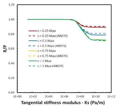
Finally, the effects of interface parameters $(k_s,c)$ on the load attenuation induced by friction along the inclusion are investigated. The load attenuation level can be defined by ratio $R/P$, that is the ratio between axial load at the inclusion fixed end and applied load at the inclusion free end. Figure 11 displays for each value of interface cohesion variations of load attenuation as a function of interface stiffness. The good agreement of the model predictions with ANSYS finite element solutions should first be emphasized. Corroborating the comments formulated previously, some qualitative features regarding the structural response can be also underlined:

• The interface condition slightly affects the attenuation load as long as $k_s\le \text{1}{0}^7\text{Pa}/\text{m}$.

• There exists a threshold value for interface cohesion beyond which the load attenuation remains unchanged, as suggested by the perfect identity observed for the $c=0.75\text{MPa}$ predicted curve and the $c=1.0\text{MPa}$ predicted curve.

Figure 11
Influence of interface tangential stiffness and cohesion on load attenuation.

5 NUMERICAL APPLICATIONS

The numerical model is applied to analyze loads transfer in undrained conditions along a mooring line embedded in soil and used in petroleum exploitation units.

5.1 Problem description

Mooring systems are basically composed by mooring lines and anchors, which are responsible for maintaining floating platforms attached to the exploitation site. Special anchorage devices, such as the torpedo anchor (see Wodehouse et al. (2007) and Souza et al. (2011) for a more detailed information), have been developed for oil extraction in deep waters, where fixed anchoring points are utilized to connect the mooring lines to the anchors. In catenary mooring configuration, the suspended length of mooring line in the seawater assumes the typical shape of a free hanging line, reaching the touchdown point on the seabed surface horizontally. The final segment of the mooring lines lies embedded in the soil, comprehending the touchdown point and the anchoring point located at some position on the anchorage device. This embedded segment is usually represented considering an inverse catenary curve.

From a mechanical viewpoint, load transfer in anchorage system may be summarized as follows. As the platform drifts horizontally with the wind action and ocean current, loads are induced to the mooring system and finally transferred to the anchor (Fig. 12). Although many anchoring devices are available, torpedo anchors have proved to be a very attractive alternative for deep water anchorage. Torpedo anchors are introduced into the seabed by free fall from a previously determined altitude immersed in the seawater. The anchorage depth is determined by soil conditions and drop height, which usually varies from 30 m to 150 m. The holding capacity of a typical torpedo anchor is basically defined by the penetration depth and soil properties.

Figure 12
Schematic representation of load transfer along mooring line (a); equivalent bar modeling the buried part of mooring line (b).

The present investigation shall be restricted to load action along a mooring line segment defined between the touchdown point located on the seabed surface and the anchoring point located at the top of a torpedo anchor. Aerodynamic and hydrodynamic loads, denoted symbolically by $F_p$, acting on the floating structure are transferred to the mooring system through fairlead points located on the platform. However, the anchor is subjected to lower loads owing to friction forces acting throughout the length of the mooring line. Therefore, the main objective of the present study is to determine the load $f_t$ applied to the anchor after dissipation produced by friction forces acting on the soil-cable interface along the buried segment of the mooring line, considering that dissipation produced in the seawater results in a load $f_{\text{b}}$ at the touchdown point (see Fig. 12), which is lower than that applied at the platform level, i.e., $f_{\text{b}}<F_p$. It should be emphasized that evaluating the load $f_t$ acting on the torpedo anchor is an important issue in design of such anchors, since its value is directly related to the undrained load capacity.

5.2 Geometry discretization aspects

The geometry model is shown in Figure 13. It typically consists of a parallelepiped volume of soil whose upper face lies on the seabed plane $y=0$. The finite element discretization is defined by means of hexahedral finite elements. The shape of the mooring line segment utilized in the present analyses is defined according to an inverse catenary curve, which corresponds to the geometrical form usually observed from field measurements and numerical predictions. The final form of the curve depends on the anchoring depth. An equivalent bar with circular cross-section is adopted here to represent mooring lines made up of chains (Fig. 12b). The inverse catenary curve, located on the vertical mid-plane as shown in Fig. 13a, is approximated using Lagrange polynomial interpolation, taking into account that a minimum number of points to define the embedded leg of the mooring line is available. As the mooring line is modeled using linear cable elements, all intersections between the discretized mooring line and the finite element mesh referring to the soil material must be obtained employing a numerical algorithm for intersection detection. The numerical scheme adopted in this work to define the cable elements may be summarized as follows:

• A specific number of points is chosen along the cable line, which are obtained using the shape of the mooring line determined from field measurements or numerical predictions. Then, Lagrange polynomials are adopted to approximate the shape of the mooring line, where the polynomial degree is specified according to the number of interpolation points initially chosen. Now, a large number of points must be created in order to discretize the interpolation curve using small straight line segments. These segments are employed to define all the intersections between the interpolation curve and element faces corresponding to the matrix material, whereas the embedded cable and matrix material are discretized using linear finite elements.

• Once the points on the interpolated curve representing the embedded cable are defined, the elements of the matrix material containing the end points of the mooring line segment are to be determined. The intersection search between the interpolation curve and the faces of matrix elements begins with that matrix element containing the first point of the interpolation curve.

• Taking into account the element containing the first point of the discretized curve, the subsequent points are covered in order to find the intersection between the interpolated curve and some face of the current matrix element. The subsequent points are tested to define whether the point is contained or not in the present element of the matrix material. The first point outside the spatial domain of the matrix element and that point immediately before are chosen to construct a straight line from which the intersection point can be obtained.

• After the first intersection point is obtained, the procedure described above is repeated considering the element of the matrix material in contact with the element face of the preceding element where the intersection occurs. The first point of the straight segment representing a cable segment is now considered as the last intersection point. The points initially defined on the interpolation curve are again covered from the point subsequent to the point outside the previous matrix element. The first point outside the present element is chosen as the last point of the straight line representing a cable segment. After all the points on the interpolation curve are covered, all the straight segments representing the mooring line will be defined.

Figure 13
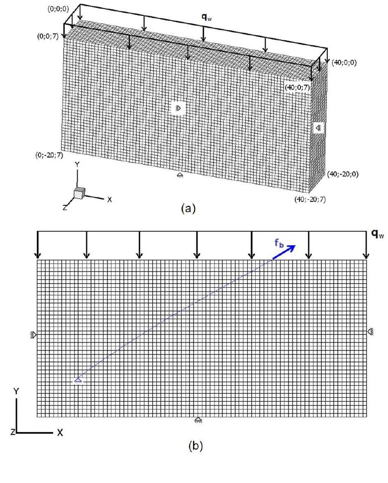
Finite element model referring to the anchoring point at 15 m depth: computational domain (a); intermediate plane containing the embedded segment of the mooring line (b).

In order to investigate the effect of the anchoring depth on the numerical predictions, three different situations have been considered, corresponding to the following anchoring depths: 15 m, 20 m and 25 m. Figure 13 illustrates the finite element discretization referring to the anchoring point at h=15 m depth, where the spatial domain related to the surrounding soil material and the discretized mooring line segment can be identified. The computational domain extends over a hexahedral volume with 20 m height, 40 m length and 7 m width. These dimensions were chosen in order to avoid the influence of boundary effects over the present results. The finite element mesh consists of 44800 eight-node hexahedral elements, which are uniformly distributed over the computational domain. Similar characteristics have been considered for the finite element meshes referring to the anchoring points at h=20 m and h=25 m using 72000 and 109200 eight-node hexahedral elements, respectively. Smooth-wall boundary conditions are imposed on the bottom and lateral surfaces of the domain geometry. On the upper surface, a hydrostatic load $q_w$ that stands for the seawater pressure acting at the seabed level (depth H=2135 m from sea level) is applied.

As mentioned previously, the curvilinear bar representing the embedded segment of the mooring line is located on the intermediate vertical plane (z = 3.5 m) of the computational domain. The anchoring point at the end of the embedded mooring line segment is modeled considering that the anchor is a rigid body with all degrees-of-freedom restricted. Hence, the anchor and the soil-anchor interface are not considered in the present approach. The lower end of the cable is positioned according to the anchoring depths analyzed here, where all the displacement degrees-of-freedom are restrained to simulate the connection between the mooring line and the torpedo anchor. On the other hand, the upper end is located on the seabed surface, where an axial load is applied representing the aerodynamic and hydrodynamic forces acting on the floating platform, and transmitted from the fairlead to the touchdown point through the immersed segment of the mooring line in the seawater. The inverse catenary shapes referring to the different anchoring depths analyzed in this work can be approximated with the following polynomial functions, according to the anchoring depth h:

$y(x)=-15+0.7939x-0.0117x^2+0.0003x^3-2\text{x}{10}^{-6}{x}^4\text{for}\text{h=15 m}$ (84)

$y(x)=-20+0.9791x-0.019x^2+0.0004x^3-4\text{x}{10}^{-6}{x}^4\text{for}\text{h=20 m}$ (85)

$y(x)=-25+1.2323x-0.0304x^2+0.0007x^3-7\text{x}{10}^{-6}{x}^4\text{for}\text{h=25 m}$ (86)

These functions are obtained from least square fitting applied on typical data obtained from mooring systems installed in Brazilian offshore fields.

5.3 Model data

A main purpose of the analysis is to investigate the mechanical response of soil/mooring cable system under undrained loading conditions. In the context of total stress constitutive behavior, the soil is assumed to be elastic perfectly plastic with isotropic physical properties evolving with depth. A Tresca-like plasticity model is adopted for plasticity with undrained shear strength profile:

$S_u\left(y\right)=\alpha \left|y\right|$ (87)

which means that $S_u$ linearly increases with depth. Parameter $\alpha$ [Pa/m] can be evaluated from field tests like Cone Penetration Test. As regards the soil elastic properties, the Young modulus is considered to evolve with depth according to:

$E(y)=\beta S_u\left(y\right)$ (88)

$\beta$ being a dimensionless parameter (stiffness ratio) whose typical value ranges from 100 to 500 for normally consolidated soils.

The behaviors of mooring cable and related soil contact interface have been described in sections 2.2 and 2.3. The equivalent bar with circular cross-section, which is adopted in the present analysis to model the mooring line (see Fig. 12b), is considered as elastic with axial rigidity defined by the product $E_c\times A_c$. The elastic-plastic behavior of the soil/inclusion interface is defined by normal and tangential stiffness moduli $k_n$ and $k_s$, together with cohesion $c$, friction angle $\varphi$ and dilatancy angle $\psi$.

Table 3 summarizes the reference values adopted here to define the mechanical properties for the seabed soil material, the soil-cable interface and the cable model representing the embedded mooring line segment.

Table 3
Reference mechanical properties used in the numerical model.

Properties		Values
Soil	Undrained shear strength $S_u\left(y\right)=\alpha \left|y\right|$	$\alpha =1.4\text{kPa/m}$
	Elastic modulus $E(y)=\beta S_u\left(y\right)$	$\beta =300$
	Poisson ratio	$\nu =0.495$
	Saturated specific weight	$\gamma =15.1{\text{kN/m}}^{\text{3}}$
Mooring cable	Equivalent bar diameter	$d_c=0.24\text{m}$
	Axial rigidity	$E_c{A}_c=\text{1}.\text{1}\times \text{1}{0}^{\text{6}}\text{kN}$
Soil-cable interface	Tangential stiffness modulus	$k_s=\text{2}.\text{43}\times \text{1}{0}^3\text{kPa}/\text{m}$
	Normal stiffness modulus	$k_n=\text{1}{0}^6\times k_s$
	Cohesion	$c=0\text{kPa}$
	Internal friction angle	$\varphi ={30}^{\circ }$
	Dilatancy angle	$\psi =0^{\circ }$

Apart from gravity, further loading components shall be detailed in the sequel. The deep seawater pressure acting at the seabed level is fixed to $q_w=2.135\times {10}^4\text{kPa}$, corresponding to a seabed depth of about $H=2135\text{m}$.

An important aspect of the analysis is related to the initial stress distribution in the soil, i.e., the stress state prior to the application of structural load applied by the floating structure and transferred to anchor through the buried mooring cable. A comprehensive approach would theoretically rely on the analysis of whole torpedo anchor penetration process in the soil, which falls beyond the scope of the present investigation. Instead, it is assumed that the structure is loaded by the soil stress state undisturbed by the anchor installation process. More precisely, the following simplified expression for initial stress distribution is considered:

${\sigma }_v^0=\gamma y-q_w;{\sigma }_h^0=K_0{\sigma }_v^0$ (89)

where ${\sigma }_v^0={\sigma }_{yy}$and ${\sigma }_h^0={\sigma }_{xx}={\sigma }_{zz}$ are the horizontal and vertical stress components of the initial stress state. Parameter $K_0$ is similar to the coefficient of lateral earth pressure at rest, and value $K_0=1$ is considered for most of subsequent numerical simulations.

The last component of loading mode considered in the present analysis is the structural load originating from the floating platform and transferred to the anchor system defined by soil - embedded mooring cable - interface. The load is modeled by means of an axial force $f_{\text{b}}$ applied to the upper extremity of buried mooring cable, which corresponds to the touchdown point located on the seabed surface ($y=0$) (see Fig. 13a). A typical load record referring to mooring lines installed in Brazilian offshore fields shown in Fig. 14a will be considered in the numerical simulations. The corresponding spectral frequency density function is displayed in Fig. 14b, showing that the main frequencies associated with the load record are ranging around $0.002\text{Hz}$. Note also that the mean load value is approximately $f_{\text{b}}{}^{mean}\approx 4000\text{kN}$.

Figure 14
Typical load record (a); and associated spectral density function (b).

5.4 Preliminary numerical simulations

Two series of preliminary numerical calculations were undertaken with the objective to qualitatively: (a) assess whether the inertial effects induced by applied load $f_{\text{b}}$ would significantly affect, or only marginally, the mechanical response of the system constituted by cable, surrounding soil and related contact interface; and (b) provide insight into the role of interface tangential stiffness in load attenuation along embedded cable.

5.4.1 Spectral density of considered mechanical system

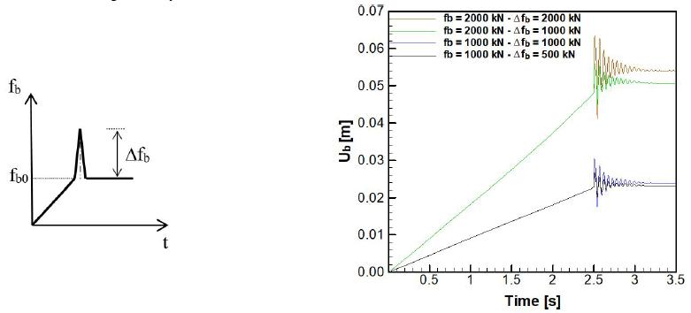
As mentioned above, a dynamic analysis aimed to evaluate the response of the mechanical system under free vibration is first performed. Fixing the anchoring point at $\text{h=15 m}$ depth, which correspond to computational domain displayed in Fig. 13, the loading process consists in applying an initial quasi-static axial load $f_{\text{b}}=f_{\text{b0}}$ at the free end of the mooring cable, followed by impulse loads of magnitude $\Delta f_{\text{b}}=f_{\text{b0}}/2$ or $\Delta f_{\text{b}}=f_{\text{b0}}$ (Fig. 15a). Figure 15b illustrates the structural response in terms of axial displacement obtained at the cable free end (loaded point) for $f_{\text{b0}}=f_{\text{b}}{}^{mean}/4$ and $f_{\text{b0}}=f_{\text{b}}{}^{mean}/2$. The frequency spectral density function can be finally defined considering the structural responses of the cable model over time, which must be compared with the spectral density function obtained from time histories referring to the load applied to the mooring line and shown in Fig. 14.

Figure 15
Schematic representation of applied load and associated structural response in terms of axial displacement.

The spectral density function obtained from the numerical simulations carried out herein is shown in Figure 16. It is observed from this analysis that the main frequencies of the mechanical system are around$20\text{Hz}$, thus indicating that the main frequencies associated with the dynamic load applied to the system are much lower than those of the system cable-surrounding soil-contact interface.

This preliminary analysis suggests that although the mooring system is subjected to dynamic forces, the mechanical response of the system can be evaluated by means of numerical simulations disregarding inertial effects, i.e., considering that loads are applied under quasi-static conditions.

Clearly enough, this conclusion has been drawn in light of calculations performed with a fixed model data. Further simulations based on a parametric study by varying several problem parameters would be necessary to corroborate this result.

Figure 16
Spectral density function obtained from dynamic simulations.

5.4.2 Effects of interface tangential stiffness on load attenuation

One important component of the model is the tangential stiffness $k_s$of the cable/soil interface, since its value is expected to strongly affect the value of load $f_t$ applied to torpedo at the anchoring point. Based on the results of the previous section, the analysis is achieved disregarding the inertial effects (i.e., quasi-static analysis).

Figure 17
Load ratio $f_t/f_{\text{b}}$ as a function of the interface tangential stiffness $k_s$.

More precisely, the investigation aims to determine the effects of cable-soil interface stiffness regarding the load attenuation along the buried mooring line. Considering the reference model data of Table 3 and fixing the anchoring point at $\text{h=15 m}$ depth (see Fig. 13), several simulations were performed varying the value of tangential stiffness values $k_s$. The analysis consisted in applying incrementally an axial load $f_{\text{b}}=f_{\text{b}}{}^{mean}$ at the free end of the cable model and to compute the reaction force $f_t$ at the anchoring point when the total load is reached. Figure 17 presents the load ratio $f_t/f_{\text{b}}$ as a function of the tangential stiffness $k_s$, the load attenuation being defined as $1-f_t/f_{\text{b}}$. It is first observed that, for considered model data, $f_t/f_{\text{b}}$ remains close to unity while $k_s\le \text{1}{0}^2\text{kPa}/\text{m}$, followed by an abrupt drop in load ratio in the interval $\text{1}{0}^2\text{kPa}/\text{m}\le k_s\le \text{1}{0}^4\text{kPa}/\text{m}$. This kind of curve suggests the existence of a stiffness range for which the load attenuation remains small with a free slip-like behavior, and a stiffness range for which the interface acts like a perfect adherent one inducing significant load attenuation. The transition zone is characterized by a high sensitivity of load $f_t$ to stiffness variation, underlying the crucial role of this parameter in the structure response. It should be kept in mind, however, that this parameter is not commonly available from field or experimental measurements.

5.5 Further simulations

Referring to model data of Table 3, simulations with different anchoring point depths are performed to evaluate the load $f_t$ applied to the torpedo anchor, as well as associated load attenuation induced by friction along the soil/cable interface. Three configurations corresponding to anchoring points located at depths $\text{h=15 m}\text{, 20 m and 25 m}$, are investigated. Axial load $f_{\text{b}}$ obtained from spectral filtering applied to the load record presented in Fig. 14a is applied at the free end of the mooring cable. This procedure leads to an equivalent load record with a smaller time interval.

Figures 18 presents for each anchoring point depth the value of load $f_t$ versus time, together with the applied load history $f_{\text{b}}$. Table 4 presents the corresponding load attenuation values obtained from the numerical simulations. As expected, the magnitude of load attenuation increases with anchoring depth.

Figure 18
Applied load history $f_{\text{b}}$ and numerically predicted load $f_{\text{t}}$ at the anchoring point for three different anchoring depths.

Table 4
Load attenuation as function of the anchoring depth.

Anchoring depth	Average attenuation	Attenuation at the load peak
15 m	20.7%	23.5%
20 m	24.6%	26.4%
25 m	26.8%	27.9%

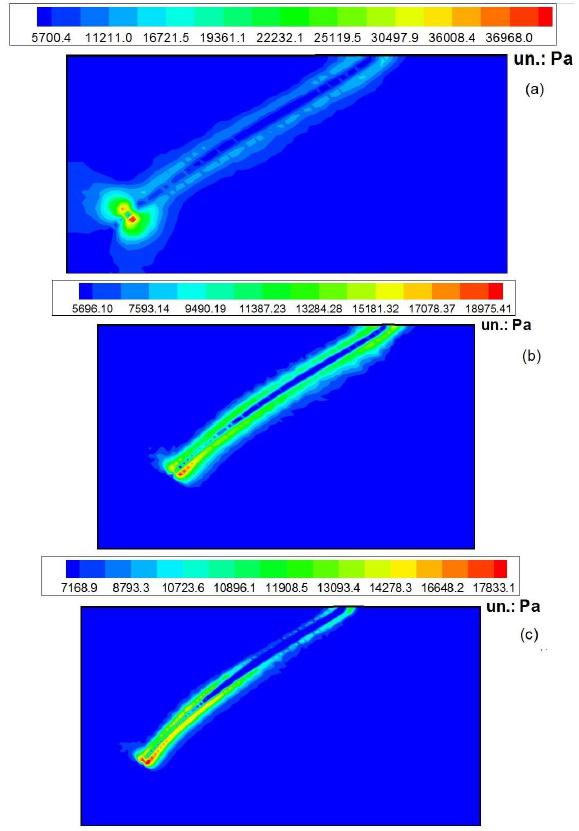
The effect of stress yielding induced by the presence of embedded cable on surrounding soil can be qualitatively assessed by visualization of the von Mises equivalent stress contours (Fig. 19). It is observed from these figures that the higher is the anchoring depth, the lower is the surrounding soil yielding (i.e., decreasing von Mises equivalent stress).

Figure 19
Contours of von Mises equivalent stress: anchoring point at 15 m depth (a); anchoring point at 20 m depth (b); anchoring point at 25 m depth (c).

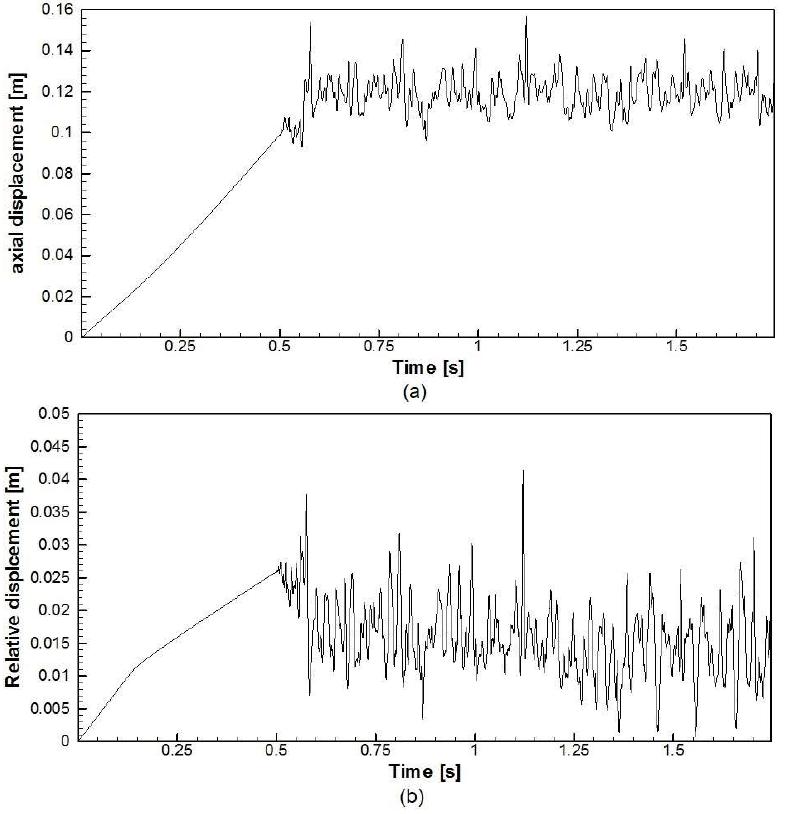
The structural response is also evaluated through axial displacement and soil/cable relative displacement at the free end of the cable. For illustrative purposes, Figures 20a and 20b show the evolution in time of these quantities in the particular case of anchoring point at $\text{h=15 m}$. Some statistical values referring to the structural response obtained in the present analysis are summarized in Table 5.

Figure 20
Structural response evaluated at the free end of the cable: axial displacement (a); relative displacement (b).

Table 5
Statistical results referring to the structural response of the cable model.

Displacements	Average value	Value at the load peak
Axial displacement	0.119 m	0.157 m
Relative displacement	0.0159 m	0.0414 m

The last series of simulations investigate the effects of soil stiffness on the load attenuation evaluated at the anchoring point. Recalling that the Young´s modulus of soil is evaluated from undrained shear strength profile $S_u$ through Eq. (88), two values of stiffness ratio, namely $\beta =300$and $\beta =500$, were considered. The depth of anchoring point is fixed to $\text{h=15 m}$.

Figure 21 shows the results obtained for load $f_t$ acting on anchoring point, together with load $f_b$applied at the free end of the cable. Table 6 gives some statistical results corresponding to the attenuation values obtained from the present load evaluations, showing that the magnitude of load attenuation is moderately affected by the soil stiffness when compared to the influence of interface stiffness.

Figure 21
Applied load history $f_{\text{b}}$ and numerically predicted load $f_t$evaluated at the anchoring point for two different values of soil stiffness.

Table 6
Load attenuation as function of the soil stiffness.

Soil stiffness	Average attenuation	Attenuation at the load peak
E(z) = 300 Su(z)	20.7%	23.5%
E(z) = 500 Su(z)	23.2%	26.9%

6 CONCLUSIONS

A mixed 3D-1D finite element formulation for structural analysis of solids with embedded curvilinear inclusions with account for interface behavior has been presented in the context of elastoplasticity. The analysis focused on the specific situation of a geomaterial surrounding bar-like inclusions that are assumed to take only tensile-compressive forces. The embedded approach together with a corotational kinematics description is adopted for nonlinear analysis of such geo-structures.

The numerical implementation of the model to investigate the problem of load transfer in mooring anchor systems has demonstrated its aptitude to deal with and macroscopically capture essential features of deformation in a complex structure. Although the simulations have mainly concerned quasi-static analyses, the current version of finite element tool can be adopted for dynamic analyses. However, such analyses handled in 3D setting require developing more efficient computational strategies including remeshing procedure and parallel computing.

From both theoretical and numerical viewpoints, several fundamental issues should be foreseen in the future. In particular:

• Development of a mechanically consistent method to properly model the interaction forces at the soil/cable interface, in the spirit of the multiphase approach proposed in Figueiredo et al. (2013).

• Formulation of the interface constitutive behavior in the context of large strains, that is to address large relative displacements between embedded inclusion and surrounding matrix. It is well know that such a task is complex regarding the finite element implementation.

• Extension of the model formulation to the situation of porous media. At the macroscopic scale, the hydromechanical coupling in soils, and more generally in geomaterials, can be account for in the framework of infinitesimal or finite poroplasticity. This is an essential aspect for addressing problems connected with geotechnical or petroleum engineering. This issue is actually the object of current developments.

As mentioned above, dynamic analyses in 3D nonlinear setting involve large computational cost. This includes parallel implementation of the finite element model with specific data structure storage and iterative solver.

Acknowledgements

The authors would like to thank CNPq (Brazilian council of research) for the financial support.

References

• Balakrishnan, S., Murray, D.W. (1986). Finite element prediction of reinforced concrete behavior. Struct. Engrg. Rep. nº 138, University of Alberta, Edmont, Alberta, Canada.
• Barzegar, F., Manddipudi, S. (1994). Generating reinforcement in FE modeling of concrete structures. Journal of Structural Engeneering, ASCE 120(5): 1656-1662.
• Bathe, K.J. (1996). Finite Element Procedures, Prentice Hall, New Jersey.
• Bennis, M., de Buhan, P. (2003). A multiphase constitutive model of reinforced soils accounting for soil-inclusion interaction behaviour. Mathematical and Computer Modelling 37: 469-475.
• Bernaud, D, de Buhan, P, Maghous, S, (1995). Numerical simulation of the convergence of a bolt-supported tunnel through a homogenization method. Int. J. Numer. Anal. Meth. Geomech. 19(4): 267-288.
• Bernaud, D., Deudé, V., Dormieux, L., Maghous, S., Schmitt, D.P. (2002). Evolution of elastic properties in finite poroplasticity and finite element analysis. International Journal for Numerical and Analytical Methods in Geomechanics 26(9): 845-871
• Bernaud, D., Dormieux, L., Maghous, S. (2006). A constitutive and numerical model for mechanical compaction in sedimentary basins. Computers and Geotechnics 33(6-7): 316-329.
• Bernaud, D., Maghous, S., de Buhan, P., Couto, E. (2009). A numerical approach for design of bolt-supported tunnels regarded as homogenized structures. Tunnelling and Underground Space Technology 24(5): 533-546.
• Braun, A.L., Awruch, A.M. (2008). Geometrically non-linear analysis in elastodynamics using the eight-node finite element with one-point quadrature and the generalized-a method. Lat. Am. J. Solids Struct. 5: 17-45.
• Braun, A.L., Awruch, A.M. (2013). An efficient model for numerical simulation of the mechanical behavior of soils. Part 1: theory and numerical algorithm. Soils & Rocks 36: 159-169.
• de Buhan, P., Sudret, B. (1999). A two-phase elastoplastic model for unidirectionally-reinforced materials. Eur. J. Mech. A/Solids 18: 995-1012.
• de Buhan, P., Bourgeois, E., Hassen, G. (2008). Numerical Simulation of bolt-supported tunnels by means of a multiphase model conceived as an improved homogenization procedure. Int. J. Numer. Anal. Meth. Geomech. 13(32): 1597-1615.
• Chang, T.Y., Taniguchi, H., Chen, W.F. (1987). Nonlinear finite element analysis of reinforced concrete panels. Journal of Structural Engineering 113(1): 122-140.
• Degenkamp, G., Dutta, A. (1989). Soil resistances to embedded anchor chain in soft clay. Journal of the Geotechnical Engineering Division 115(10): 1420-143.
• Dormieux, L., Maghous, S. (1999). Poroelasticity and poroplasticity at large strains. Oil&Gas Science and Technology - Revue de l’IFP 54(6): 773-784.
• Duarte Filho, L.A., Awruch, A.M. (2004). Geometrically nonlinear static and dynamic analysis of shells and plates using the eight-node hexahedral element with onepoint quadrature. Finite Elem. Anal. Des. 40: 1297-1315.
• Elwi, A., Hrudey, M. (1989). Finite element model for curved embedding reinforcement. Journal of Engng. Mech. (ASCE) 115(4): 740-757.
• Espath, L.F.R., Braun, A.L., Awruch, A.M., Maghous, S. (2014). NURBS-based three-dimensional analysis of geometrically nonlinear elastic structures. Eur. J. Mech. A/Solids 47: 373-390.
• Felippa, C.A., Haugen, B. (2005a). A unified formulation of small-strain corotational finite elements: I. Theory. Comput. Methods Appl. Mech. Eng. 194: 2285-2336.
• Felippa, C.A., Haugen, B. (2005b). Unified Formulation of Small-strain Corotational Finite Elements: I. Theory. Technical report n° cu-cas-05-02. Center for Aerospace Structures, University of Colorado, Colorado, USA.
• Figueiredo, M.P., Maghous, S., Campos Filho, A. (2013). Three-dimensional finite element analysis of reinforced concrete structural elements regarded as elastoplastic multiphase media. Materials and Structures 46(3): 383-404.
• Gomes, H.M., Awruch, A.M. (2001). Some aspects on three-dimensional numerical modeling of reinforced concrete structures using the finite element method. Advances in Engineering Software 32: 257-277.
• Hassen, G., de Buhan, P. (2006). Elastoplastic multiphase model for simulating the response of piled raft foundations subject to combined loadings. Int. J. Numer. Anal. Meth. in Geomech. 30: 843-864.
• Hassen, G., Gueguin, M., de Buhan, P. (2013). A homogenization approach for assessing the yield strength properties of stone column reinforced soil. Eur. J. Mech. A/Solids 37: 266-280.
• Hughes, T., Winget, J. (1980). Finite rotations effects in numerical integration of rate constructive equations arising in large deformation analysis. Int. J. Numer. Methods Eng. 15: 1862-1867.
• Laursen, T.A. (2010). Computational Contact and Impact Mechanics. Springer-Verlag Berlin Heidelberg.
• Maghous, S., Bernaud, B., Couto, E. (2012). Three-dimensional numerical simulation of rock deformation in bolt-supported tunnels: a homogenization approach. Tunnelling and Underground Space Technology 31: 68-79.
• Manzoli, O.L., Oliver, J., Diaz, G., Huespe, A.E. (2008). Three-dimensional analysis of reinforced concrete members via embedded discontinuity finite elements. Revista Ibracon de Estruturas e Materiais 1: 58-83.
• Nayak, G.C., Zienkiewicz, O.C. (1972). Elasto-plastic stress analysis. A generalization for various constitutive relations including strain softening. International Journal for Numerical Methods in Engineering 5: 113-135.
• Neubecker, S.R., Randolph, M.F. (1995). Profile and frictional capacity of embedded anchor chains. Journal of the Geotechnical Engineering Division 121(11): 797-803.
• Ninic, J., Stascheit, J., Meschke, G. (2014). Beam-solid contact formulation for finite element analysis of pile-soil interaction with arbitrary discretization. International Journal for Numerical and Analytical Methods in Geo mechanics 38: 1453-1476.
• Oliver, J., Diaz, G., Huespe, A.E., Manzoli, O.L. (2008). Two-dimensional modeling of material failure in reinforced concrete by means of a continuum strong discontinuity approach. Comput. Methods Appl. Mech. Engrg. 197: 332-348.
• Owen, D.R.J., Hinton, E. (1980). Finite Elements in Plasticity: Theory and Pratice. Pineridge Press: Swansea, UK.
• Phillips, D.V., Zienckiewicz, O.C. (1976). Finite element non-linear analysis of concrete structures. Proc. Instit. Civ. Engrs., Part 2, 61(3): 59-88.
• Ranjbaran, A. (1996). Mathematical formulation of embedded reinforcements in 3D brick elements. Commun. Num. Methods Engng 12: 897-903.
• Sadek, M., Shahrour, I. (2004). A three dimensional embedded beam element for reinforced geomaterials. Int. J. for Num. Anal. Methods in Geom. 28(9): 931-946.
• Souza, J.R.M., Aguiar, C.S., Ellwanger, G.B., Porto, E.C., Foppa, D., Medeiros Junior, C.J. (2011). Undrained Load Capacity of Torpedo Anchors Embedded in Cohesive Soils. J. Offshore Mech. Arctic Engng. 133(2), 021102, (12 pages).
• Souza Neto, E.A., Peric´, D., Owen, D.R.J. (2008). Computational Methods for Plasticity: Theory and Applications. John Wiley & Sons, Chichester, UK.
• Sudret, B., de Buhan, P. (2001). Multiphase model for inclusion-reinforced geostructures application to rock-bolted tunnels and piled raft foundations. International Journal for Numerical and Analytical Methods in Geomechanics 25: 155-182.
• Wang, L., Guo, Z., Yuan, F. (2010a). Three-dimensional interaction between anchor chain and seabed. Applied Ocean Research 32: 404-413.
• Wang, L., Guo, Z., Yuan, F. (2010b). Quasi-Static ThreeDimensional Analysis of Suction Anchor Mooring System. Ocean Engineering 37: 1127-1138.
• Wodehouse, J., George, B., Luo, Y. (2007). The Development of a FPSO for the Deepwater Gulf of Mexico. Proceedings of the 39th Offshore Technology Conference, Houston, TX, Paper No. 18560.
• Wriggers, P. (2006). Computational Contact Mechanics, 2^nd Edition. Springer-Verlag Berlin Heidelberg.
• Yang, Y-B., Shieh, M-S. (1990). Solution method for nonlinear problems with multiple critical points. AIAA J. 28: 2110-2116.
• Yu, L., Tan, J.H. (2006). Numerical investigation of seabed interaction in time domain analysis of mooring cables. Journal of Hydrodynamics 18(4): 424-30.
• Zhou, Y.D., Cheuk, C.Y., Tham, L.G. (2009). An embedded bond-slip model for finite element modelling of soil-nail interaction. Computers and Geotechnics 36(6): 1090-1097.

• Available Online: June 26, 2018

Publication Dates

• Publication in this collection
  2018

History

• Received
  07 Dec 2017
• Reviewed
  11 Dec 2017
• Accepted
  19 June 2018