Abstract
The constitutive behavior of geomaterials is generally affected by the presence at different scales of discontinuity surfaces with different sizes and orientations. According to their mechanical behavior, such discontinuities can be distinguished as cracks or fractures. Fractures are interfaces that can transfer normal and tangential stresses, whereas cracks are discontinuities without stress transfer. Regarding the formulation of the behavior of materials with isotropic distribution of micro-cracks or fractures, previous works had essentially focused on their instantaneous response induced by structural loading. Few research works have addressed time-dependent (delayed) behavior of such materials. The present contribution describes the formulation and computational implementation of a micromechanics-based modeling for viscoelastic media with an isotropic distribution of micro-fractures. The homogenized viscoelastic properties are assessed by implementing a reasoning based on linear homogenization schemes (Mori-Tanaka) together with the correspondence principle for non-aging viscoelastic materials. It is shown that the homogenized viscoelastic behavior can be described by means of a generalized Maxwell rheological model. The computational implementation is developed within the finite element framework to analyze the delayed behavior of geomaterials with the presence of isotropically distributed micro-fractures under plane strain conditions. Several examples of applications are presented with the aim to illustrate the performance of the finite element modeling. The assessment of the approach accuracy and the corresponding code verification are performed by comparing the numerical predictions with analytical solutions for simple and complex geo-structures.
Keywords:
Fracture; micromechanics; viscoelasticity; finite element
1 INTRODUCTION
One of the most common causes of material degradation in civil engineering structures is the presence of discontinuity surfaces, which can appear with different sizes and orientations. The existence of these small thickness regions increases the risk of mechanical properties deterioration during the service life of structures because of a significative reduction of stiffness, strength, ductility and a serious increase of permeability. From a mechanical behavior perspective, there are two principal types of discontinuities: cracks and fractures. Essentially, cracks have no stress transfer between faces, whereas fractures can transfer normal and tangential stresses. Consequently, a medium can be considered as cracked or fractured depending on the characteristics of its discontinuities.
Geomaterials under long-term loading present two types of response: instantaneous and delayed. The instantaneous response of fractured geomaterials has been object of research over the years (see for instance Budiansky and O’Connell, 1976Budiansky B, O’Connell RJ (1976). Elastic moduli of a cracked solid.International Jounal ofSolids Structures 12: 81-97.). However, less attention has been given to delayed response in fractured mediums. Given the importance of delayed components on stress/strain response of geomaterials, researches focused on time-dependent respose addressing both fracture mechanics and viscoelasticity have been conducted recently. In order to study and characterize that behavior, several mathematical models have been analytically formulated. Among these models, there are those based on a micromechanics framework.
Some important micromechanics-based works that considered delayed behavior were developed by Nguyen et al. (2010Nguyen, S. T., Dormieux, L., Le Pape, Y., Sanhuja, J. (2010). Crack propagation in viscoelastic structures:Theoretical and numerical analyses. Computational Materials Sciences 50: 83-91., 2013) and Nguyen and Dormieux. (2014). These researchers formulated a micromechanics-based model for a viscoelastic medium where the heterogeneities are considered as cracks. However, as mentioned above, there are no stress transfer in this type of discontinuities. Subsequently, Nguyen´s analysis was extended by Aguiar and Maghous (2018Aguiar, C.B., Maghous, S., (2018). Micromechanical approach to effective viscoelastic properties of micro‐fractured geomaterials. International Journal for Numerical and Analytical Methods in Geomechanics 42(16): 2018-2046), who added the fracture behavior studied by Maghous et al. (2011).
In this context, the main objective of the present paper is related to the finite element modeling and implementation within a computational code of the viscoelastic constitutive behavior originally formulated in Aguiar and Maghous (2018Aguiar, C.B., Maghous, S., (2018). Micromechanical approach to effective viscoelastic properties of micro‐fractured geomaterials. International Journal for Numerical and Analytical Methods in Geomechanics 42(16): 2018-2046) for the fractured medium. It is emphasized that the main novelty of the approach lies in the ability of such a computational tool to allow for effective and accurate analysis of the delayed response of structures built in fractured media.
The paper content is organized as follows. Section 2 presents succinctly the theoretical formulation for the homogenized viscoelastic behavior of fractured mediums, considering an isotropic distribution of micro-fractures. Section 3 describes the algorithm used for time discretization of the viscoelastic model. Section 4 aims to verify the implementation code by presenting several examples of application where the accuracy of the numerical responses is assessed through comparison with the corresponding analytical solutions. Finally, section 5 illustrates the predictive capabilities of the computational tool by analyzing the delayed response of a complex geo-structure.
2 FORMULATION OF THE HOMOGENIZED VISCOELASTIC MODEL
As mentioned above, Aguiar and Maghous (2018Aguiar, C.B., Maghous, S., (2018). Micromechanical approach to effective viscoelastic properties of micro‐fractured geomaterials. International Journal for Numerical and Analytical Methods in Geomechanics 42(16): 2018-2046) formulated the homogenized viscoelastic properties for a fractured medium. This approach is based on prior research works developed within the framework of elastic fractured mediums (Maghous et al. 2011, 2014) and the elastic-viscoelastic correspondence principle in the context of non-aging materials. There are two principal steps in order to formulate the macroscopic viscoelastic properties: in first place, it is necessary to formulate the overall elastic properties of the medium taking advantage of linear homogenization schemes. The second step is to associate the elastic-viscoelastic correspondence principle (Le, 2008Le QV. (2008). Modélisation multi‐échelle des matériaux viscoélastiques hétérogènes. Application à l'identification et à l'estimation du fluage propre de béton d'enceintes de centrales nucléaires. Ph. D. Thesis (in French), Université Paris‐Est, France.) with a specific procedure to determinate the inverse Laplace-Carson transform of a function.
Since the paper focus is the study of the computational implementation of the viscoelastic model, only the formulation of the homogenized viscoelastic properties in a medium with isotropically distributed fractures will be shown below in a concise way. The formulation of the elastic properties in a fracture medium, the complete procedure of inverse Laplace-Carson transform and other basic concepts of the theoretical model can be found in Aguiar and Maghous (2018Aguiar, C.B., Maghous, S., (2018). Micromechanical approach to effective viscoelastic properties of micro‐fractured geomaterials. International Journal for Numerical and Analytical Methods in Geomechanics 42(16): 2018-2046).
2.1 Homogenized viscoelastic properties in a medium with isotropic distribution of micro-fractures
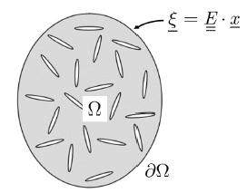
Let denote the representative elementary volume (REV) of a homogeneous material (the matrix phase) cut by a discrete distribution of randomly oriented short fractures (the embedded fractures phase). The REV is chosen so as to be statistically representative of the fractured medium and to comply with scale separation conditions (Zaoui, 2002Zaoui A. (2002). Continuum micromechanics: survey. Journal of Engineering Mechanics ASCE 128(8): 808‐816.). In particular, the characteristic size of fractures is assumed to be small with respect to the dimension of the REV, which in turn should be small when compared to a characteristic dimension of the structure body. For sake of simplicity and without loss of generality, we shall assume that the REV is a Lipschitz domain and its boundary is located in the matrix phase (i.e., does not intersect the fractures phase). As classically considered in micromechanics-based approaches, the loading of the REV can be defined by homogeneous strain type boundary conditions (Zaoui, 2002): , where represents the macroscopic strain (loading parameter), is the displacement filed and is the position vector. Figure 1 provides a schematized representation of the REV and associated loading mode.
From a constitutive viewpoint, the matrix material is assumed to exhibit a non-aging linear viscoelastic behavior defined by the fourth-order relaxation tensor . The fractures are discontinuities that are able to transfer stress and can therefore be regarded as interfaces with a specific non-aging linear viscoelastic behavior.
The formulation of non-aging viscoelastic properties of a homogenized medium involves the determination of the fourth-order relaxation tensor components. This determination relies upon the solution to a viscoelastic concentration problem stated on the REV under applied loading (Aguiar and Maghous, 2018Aguiar, C.B., Maghous, S., (2018). Micromechanical approach to effective viscoelastic properties of micro‐fractured geomaterials. International Journal for Numerical and Analytical Methods in Geomechanics 42(16): 2018-2046). In such conditions, the homogenized constitutive law for a fractured viscoelastic medium can be defined as
where is the macroscopic stress, is the strain concentration tensor associated with the viscoelastic problem defined on the REV. The fourth order tensor represents the link between the local strain at any point of the REV and applied macroscopic strain . In the above relationship, the symbol denotes the Boltzmann operator and the symbol represents the volume average over the matrix. It is pointed out that the time derivative should be understood in the sense of distributions in order to account for possible strain jumps in time. For practical determination of tensor, it is convenient to resort to the elastic-viscoelastic correspondence principle. This principle enables to formulate the time-domain viscoelastic problem in terms of an equivalent elastic problem in the Laplace-Carson domain.
In view of all the above mentioned, it is possible to take advantage of the elastic properties of a fractured medium. It should be taken into account that in the elastic problem, fractures are considered as randomly oriented oblate ellipsoids. This particular feature can be considered as an isotropic distribution of fractures in the REV as shown in Figure 1. It is also important to point out that for the determination of the homogenized stiffness tensor in the elastic problem, it was adopted the Mori-Tanaka linear homogenization scheme. The same scheme will be used for determination of the relaxation tensor in the Laplace-Carson space, which can be denoted by .
After tensor determination in Laplace-Carson domain, it becomes essential to express the relaxation tensor components in the real time domain. This raises the need for a specific inverse Laplace-Carson transform procedure , which was developed by Aguiar and Maghous (2018Aguiar, C.B., Maghous, S., (2018). Micromechanical approach to effective viscoelastic properties of micro‐fractured geomaterials. International Journal for Numerical and Analytical Methods in Geomechanics 42(16): 2018-2046). This procedure was conceived to work with the tensor obtained from a Mori-Tanaka homogenization scheme when used classical rheological models for description of matrix and fractures behavior. What follows is a summary of the main considerations of the procedure. Any non-zero component of relaxation tensor is generically referred to as . This function can be expressed as
where is the common degree of polynomials and . The variable belongs to the Laplace-Carson domain. Scalar and are real coefficients that depend on the rheological viscoelastic models adopted for matrix and fractures. By sake of simnplicity, the following steps deal with , which corresponds to function changed to the laplace domain:
The inverse Laplace transform of can be named as and the corresponding expression is
where represents the non-zero component of tensor , represent the Heaviside function at origin and the scalar is the kth root of the polynomial . In the context of macroscopic isotropy, the generic function refers to either bulk or shear relaxation moduli. The definition of the relaxation tensor in the case of randomly oriented fractures within an isotropic viscoelastic matrix and its corresponding moduli are presented in (5).
where the subscripts and indicate that the parameters and are referring to the relaxation behavior in bulk and relaxation behavior in shear, respectively. The fourth-order tensors and are the spherical and deviatoric tensors, respectively. These tensors can be defined as and , where is the fourth-order unitary tensor.
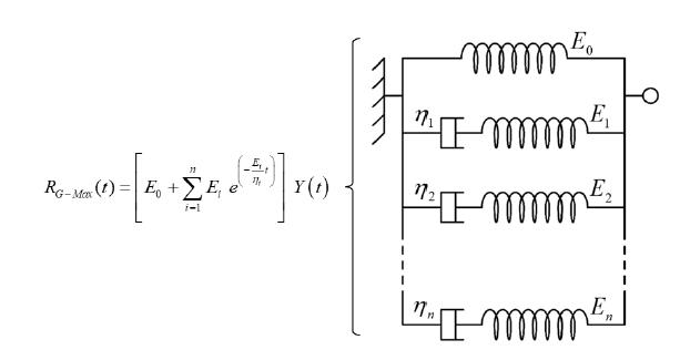
Comparing Eq. (4) with the relaxation function of a Generalized Maxwell rheological model in Figure 2, it is noticed that exist a mathematical equivalence between them. From this equivalence, it can be stated that the mentioned rheological model represents the delayed behavior of non-aging linear viscoelastic materials and, therefore, it can be considered as the exact viscoelastic model. It should be emphasized that such a mechanical analogy results from direct application of the homogenization procedure (Aguiar and Maghous, 2018Aguiar, C.B., Maghous, S., (2018). Micromechanical approach to effective viscoelastic properties of micro‐fractured geomaterials. International Journal for Numerical and Analytical Methods in Geomechanics 42(16): 2018-2046), without any a priori simplifying assumption that would be introduced to lead this analogy.
Generalized Maxwell model and its relaxation function (excerpt from Aguiar and Maghous, 2018Aguiar, C.B., Maghous, S., (2018). Micromechanical approach to effective viscoelastic properties of micro‐fractured geomaterials. International Journal for Numerical and Analytical Methods in Geomechanics 42(16): 2018-2046)
In the case of macroscopic isotropy, it is deduced that the bulk and shear viscoelastic behavior in (5) can also be exactly represented by a Generalized Maxwell rheological model, as displayed in Figure 3.
Generalized Maxwell model for viscoelastic moduli and (excerpt from Aguiar and Maghous, 2018Aguiar, C.B., Maghous, S., (2018). Micromechanical approach to effective viscoelastic properties of micro‐fractured geomaterials. International Journal for Numerical and Analytical Methods in Geomechanics 42(16): 2018-2046)
As seen in Eq. (5), for an isotropic distribution of randomly oriented fractures, tensor depends on the moduli and . In this way, taking advantage of the elastic-viscoelastic correspondence principle, viscoelastic moduli and in Laplace-Carson domain must be obtained in order to apply subsequently the inverse Laplace-Carson transform. The expressions for these viscoelastic moduli in Laplace-Carson domain are shown in (6).
where is the fracture density parameter, is the number of fractures per unit volume and is the radius of the oblate fracture. The dimensionless functions and are defined as
where parameters and depend on the rheological model adopted for the viscoelastic behavior of the constituents (matrix and fractures). As mentioned above, having defined the moduli and , it only remains to apply the inverse Laplace-Carson transform procedure in order to obtain the moduli in time domain: and .
3 ALGORITHM FOR TIME DISCRETIZATION OF THE VISCOELASTIC MODEL
In the previous section, it was defined the theoretical formulation of the homogenized viscoelastic model for geomaterials with isotropically distributed micro-fractures. Now, it is necessary to develop a numerical programming scheme which considers a time discretization in the finite element framework. Essentially, what needs to be implemented is the viscoelastic constitutive law that describes the material behavior when applied a homogeneous strain boundary condition.
Based on the conditions mentioned above, subroutines to be generated will be responsible for the calculation of homogenized stresses at Gauss points in finite element mesh of the analyzed structure. It is important to emphasize that the finite element approach is performed at the macroscopic scale in which the fractured medium is replaced by the homogenized viscoelastic material determined from previous micromechanical reasoning. In other words, the finite element discretization refers to the structure regarded as a homogenized structure. In this respect, the Greek letters used for denote stress and strain macroscopic tensors will be and , respectively.
The relaxation tensor for an isotropic distribution of microfractures, as well as the corresponding viscoelastic moduli and were defined in (5). It must be emphasized that numerical expressions for the viscoelastic moduli are previously obtained by any calculus software. Thus, these moduli are considered as input data for the program. In this way, the relaxation tensor can be expressed in matrix form as
Once the relaxation tensor is computed, the macroscopic stress tensor can be determined, according to the constitutive law, as follows
where is the instantaneous strain tensor that appears right in the moment of load application.
Regarding the code development, it will be considered time steps with the same size and . For the time step, the corresponding time can be defined as
An incremental procedure is applied in the integral equation in (9). Thus, the stress tensor at time , is
A linear variation is assumed for the strain in the interval where the variable of integration . This assumption allows to express the derivative as
In order to update the stress tensor equation, (12) is replaced in (11). In a summarized form, the stress tensor can be expressed as
where and are fourth-order tensors defined as
At this point, it must be remembered that the relaxation function for a Generalized Maxwell rheological model have mathematical equivalence with the relaxation tensor components and it can be expressed in a generic way as
where stands for the stiffness of spring model. and are, respectively, the elastic spring stiffness and dashpot viscosity of branch and is the total number of branches. Since tensors and depend on tensor , their components can be conveniently expressed as
It is known that in an isotropic distribution of fractures, for the non-zero components of tensor , the following applies
The same equalities shown in (17) applies also to tensors and . Now, considering (5), it can be determined the expressions for non-zero components of tensor
Similarly, for tensor , the corresponding non-zero components are
where corresponds to the bulk relaxation modulus and to the shear relaxation modulus.
The precedent expressions make possible the stress calculation at Gauss point for all the considered step times. According to the way the stress tensor was formulated in (13), it is proposed to define the stress tensor components for three different time steps: TS = 1, TS = 2 and TS ≥ 3.
For TS = 1, where and , the stress tensor can be defined as:
where and is the homogenized relaxation tensor evaluated at TS = 1. It is known that is the instantaneous strain tensor. The matrix form of tensor is found in (25).
For TS = 2, where and , the stress tensor can be defined as
where and is the homogenized relaxation tensor evaluated at TS = 2. is the tensor evaluated at TS=1 (). The matrix form of tensor is found in (27).
For TS ≥ 3, where , and , the stress tensor can be defined as:
The matrix form of tensor for TS ≥ 3 is presented in (29).
where SAE11, SAE22, SAE33 and SAE12 are defines as
Finally, expressions (25), (27) and (29) can be considered as the basis for the implementation code.
4 VERIFICATION OF THE IMPLEMENTATION CODE
This section is focused on the verification of the implementation code through the analysis of two examples of application under plane strain conditions. Each one of them presents a time-dependent analytical solution that will be compared with the corresponding numerical responses. The correspondence between the delayed responses will serve to verify the developed code.
The same specimen will be used for the two examples. With respect to the specimen dimensions, it is a square with a size of 1.00 m. As regards the discretized geometry model, it is composed of four square finite elements, even though it is possible to use just one finite element since stress and strain fields are homogeneous for all these examples. Figure 4 displays the finite elements, nodes and dimensions of the geometric model.
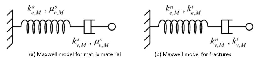
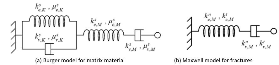
With regard to viscoelastic characteristics of the material, the related parameters depend on the rheological model chosen to describe matrix and fractures behaviors at microscopic scale. The general case considers a Burger rheological model for representation of the matrix and fractures delayed behavior. However, for the examples in this paper, it will be analyzed two particular cases of viscoelastic behavior. These two cases combine rheological models adopted by the material constituents. In the first case, matrix and fractures adopt a Maxwell rheological model, while in the second case, matrix adopt a Burger rheological model and fractures adopt a Maxwell rheological model.
Figures 5 and 6 display, respectively, the rheological model elements and their corresponding parameters for case 1 and 2. Tables 1 and 2 show, respectively, the mechanical parameters used for matrix and fractures. These parameters were reported in Le (2008Le QV. (2008). Modélisation multi‐échelle des matériaux viscoélastiques hétérogènes. Application à l'identification et à l'estimation du fluage propre de béton d'enceintes de centrales nucléaires. Ph. D. Thesis (in French), Université Paris‐Est, France.) for viscoelastic moduli of concrete, in Bart (2000Bart, M. (2000). Contribution à la modélisation du comportement hydromécanique des massifs rocheux avec fractures, Ph.D. Thesis (in French), Université Lille 1, France.) for elastic fracture behavior and the viscosity parameters of fractures were arbitrarily chosen according to Aguiar and Maghous (2018Aguiar, C.B., Maghous, S., (2018). Micromechanical approach to effective viscoelastic properties of micro‐fractured geomaterials. International Journal for Numerical and Analytical Methods in Geomechanics 42(16): 2018-2046). The fracture density parameter is and the number of fractures per unit volume .
Burger model is composed by a Maxwell component (subscript M) connected in series with a Kelvin component (subscript K). With respect to matrix material, elastic parameters associated with a spring in bulk are denoted by and , whereas that associated in shear are and . Viscosity parameters associated to a dashpot in bulk are denoted by and , whereas that associated in shear are and . As regards the fractures behavior, the elastic parameter associated with a spring under normal stress is denoted by , whereas that associated under tangential stress is . The viscosity parameter associated to a dashpot under normal stress is denoted by , whereas that associated under tangential stress is . It is emphasized that the above rheological models used for the viscoelastic behaviors of the constituents (matrix, fractures) refer to the microscopic scale, while the homogenized viscoelastic behavior is still given by (4), which reflects the behavior at macroscopic scale. In particular, the parameters associated at this scale with the generalized Maxwell model (spring stiffness and dashpot viscosity ) are calculated in each case from the viscoelastic properties of the matrix and fractures.
Comparison between analytical solutions and numerical responses for the two examples of application under plane strain conditions is presented in the following subsections.
4.1 Example 1: Plane strain compression test
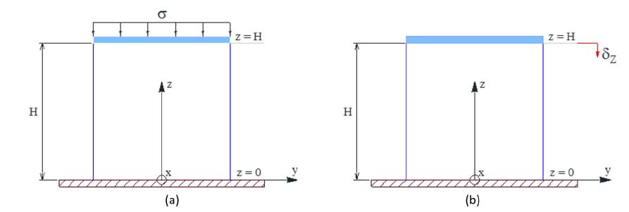
Figure 7 shows a specimen with height H subjected to two different loading cases under plane strain conditions. Figure 7A shows an imposed compressive stress , whereas Figure 7B shows a vertical imposed displacement , where denotes the Heaviside step function at origin. Material will be considered homogeneous, isotropic and linear viscoelastic. The initial stress state is .
The problem solution in both situations involves the calculation of time-dependent stress and displacement fields by using basic concepts of continuum mechanics and viscoelasticity. Once the static and kinematic admissibility of the respective solution fields for the specimen subjected to compressive stress has been determined, the analytical solution tensorial fields are
where stands for viscoelastic bulk modulus and for viscoelastic shear modulus. Variables and refer to the coordinates of position vector . These moduli are defined as
where and are the homogenized bulk and shear moduli in Laplace-Carson domain, respectively. denotes the inverse Laplace-Carson transform. These moduli depend on the rheological models adopted for representation of matrix and fractures behavior. It will be considered a compressive stress for calculations.
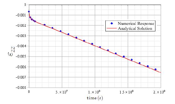
Referring to Maxwell-Maxwell case, Figures (8) and (9) are showing the comparison between the analytical solution defined in (31) and the numerical prediction for vertical strain and horizontal strain .
Similarly, the comparison between analytical solution defined in (31) and numerical response for Burger-Maxwell case are depicted in Figures (10) and (11).
As regard the error analysis, Figure (12a) and Figure (12b) plot the relative error between the analytical and numerical predictions as function of time.
The results observed from the above figures show a good agreement between the analytical and finite element solutions, exhibiting a relative error that remains lower than 6.5% for the time interval of analysis. Consequently, the implementation code has been successfully verified.
In the case of the specimen subjected to a vertical imposed displacement, the analytical solution tensorial fields are
where variables and are coordinates of the position vector . The strain caused by imposed displacement is denoted by . The bulk and shear moduli in time domain are denoted by and , respectively. The numerical expressions of and can be obtained by means of calculus softwares and depend on the rheological models adopted for matrix and fractures. It will be considered an imposed displacement for calculations.
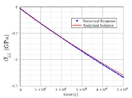
In the Maxwell-Maxwell case, Figures (13) and (14) present the comparison between analytical solution defined in (33) and numerical response for vertical stress and stress perpendicular to YZ-plane.
Similarly, comparisons between analytical solution defined in (33) and numerical response for Burger-Maxwell case are shown in Figures (15) and (16).
The variations in time of the relative error between the analytical and numerical predictions are plotted in Figures (17a) and (17b).
As shown in Figure 17, the analytical and numerical predictions show a good agreement for the early stages of analysis with increasing discrepancy with time due to the very small values of , which leads to irrelevant relative error evaluations. Once again, the implementation code has been successfully verified.
4.2 Example 2: Compression under prescribed displacement rate
Figure 18 shows a specimen with height H subjected to a constant imposed displacement rate under plane strain conditions. The applied displacement is time-dependent and can be defined as
where stands for the vertical displacement imposed at the time and denotes the Heaviside step function at origin.
Material will be considered homogeneous, isotropic and linear viscoelastic. The initial stress state will be considered as and the strain related to displacement can be expressed as
where can be considered as the vertical strain rate and as the instantaneous vertical strain.
As seen in sections 4.1 and 4.2, the problem solution involves the calculation of time-dependent stress and displacement fields by using basic concepts of continuum mechanics and viscoelasticity. Once the static and kinematic admissibility of the respective solution fields has been determined, the analytical solution tensorial fields are
where and are relaxation tensor components. The instantaneous horizontal strain can be obtained from the viscoelastic solution shown in section 4.1 for imposed displacement problem. The horizontal strain rate is:
It will be considered an imposed instantaneous displacement and a displacement rate for calculations. In relation to Maxwell-Maxwell case, Figures (19) and (20) show the comparison between analytical solution defined in (36) and numerical response for vertical stress and stress perpendicular to YZ-plane.
Similarly, comparisons between analytical solution defined in (36) and numerical response for Burger-Maxwell case is illustrated in Figures (21) and (22).
A direct error analysis is illustrated in Figure (23) by depicting the relative error between the analytical and numerical predictions obtained for the stress components along time.
The results shown in the preceding figures indicate a satisfactory agreement with a maximum relative error less than 3% along the time interval of analysis. Consequently, the implementation code has been successfully verified for all the examples presented in this section.
5 ANALYSIS OF DELAYED BEHAVIOR OF DEEP UNDERGROUND GALLERIES
The implementation code was verified in section 4 through several examples using a simple quadrilateral specimen. In addition to that verification, this section is focused on the analysis of geo-structures of greater complexity under plane strain conditions. There exist some geo-structures that allow this type of analysis, such as the deep underground galleries or tunnels. The study of these geo-structures enables to determine a cross-section of interest for carrying out a two-dimensional analysis.
It will be considered two types of cross-section for deep tunnels: circular and horseshoe. Concerning to circular cross-section, two situations will be presented: unlined cross-section and lined cross-section. In both situations related to the circular tunnel, additional verifications of the implementation code performance will be performed by comparing the analytical solution and numerical response for delayed behavior in this type of geo-structures. Subsequently, for a horseshoe cross-section, its delayed response will be analyzed in order to highlight the predictive capabilities of this computational tool when it is not possible to have an analytical solution for viscoelastic behavior.
5.1 Unlined circular cross-section tunnel
The hypotheses considered in this problem are described as follows. The tunnel has radius R and a depth H, where HR. The massif material is homogeneous and isotropic. The excavation process will be regarded as instantaneous. The initial stress (geostatic) , due to self-weight of the massif, will be uniform in the region around the gallery. The variable is defined as , where represents the specific weight of the massif and is the second-order unitary tensor. Due to symmetry determined by the tunnel geometry, only a quarter of the total structure will be used for respective analyses. The discretized geometry model consists of a 2D square domain of side length . Figure 24 displays dimensions for the numerical analysis, as well as displacement and stress boundary conditions.
The analytical solution involving delayed response will be shown in polar coordinates due to the geometric characteristics of the tunnel cross-section. Position vector does not depend on the angular coordinate and can be defined as , where is the radial distance. The problem solution involves calculation of stress and displacement fields by using basic concepts of continuum mechanics and viscoelasticity for , where is considered as the instant right after excavation. The temporal evolution of solution fields is shown as follows
where is the Heaviside function at and the modulus depends on the rheological models adopted by the matrix and fractures. This modulus can be defined as
where is the shear relaxation modulus in Laplace-Carson domain.
The radial convergence is an important parameter related to the displacements in unlined cross-sections and can be expressed as
It will be considered a depth , radius , specific weight for calculations. The lateral and vertical pressure exerted by massif is . Concerning to viscoelastic characteristics of the material, the cases of delayed behavior adopted by matrix and fractures are the same as those used in section 4: Maxwell-Maxwell and Burger-Maxwell. Consequently, mechanical parameters correspond to those specified in Tables 1 and 2, as well as the fracture density parameter and the number of fractures per unit volume . Regarding to the discretized geometric model, Figure 25 shows the finite element mesh used for the analyses. It is composed of 192 finite element and 221 nodes.
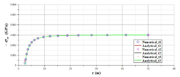
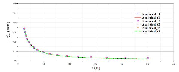
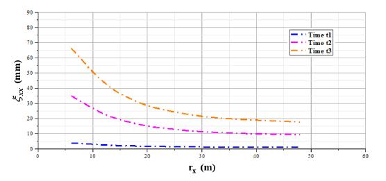
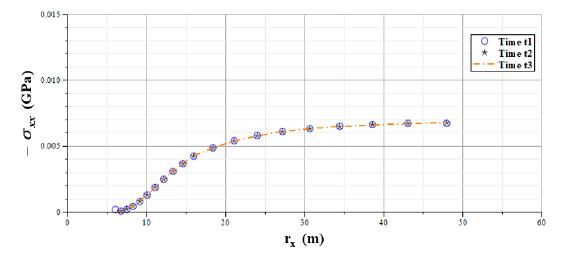
In relation to Maxwell-Maxwell case, the analytical solution, defined in (38) and (40), will be compared with the numerical response for radial convergence , radial displacement and radial stress . Regarding to radial displacements and stresses, the analysis will be performed for three different times: corresponds to the instantaneous elastic response, is an intermediate time and corresponds to a very long time.
Similarly, below is shown the comparison of analytical solution, defined in (38) and (40), with the numerical response for Burger-Maxwell case.
As shown in Figures 26- 31, analytical and numerical curves present a satisfactory correspondence. It can be considered as an additional verification of correct performance of the implementation code. Despite the consistent correspondence between analytical and numerical results, boundary effects related to displacements have been observed in Figures 27 and 30. Since boundary displacements are supposed to be zero in the discretized geometric model, it is necessary to perform future researches focused on discretized model dimensions and finite element mesh refinement in order to reduce these boundary effects.
5.2 Lined circular cross-section tunnel
The hypotheses considered in this section will be the same as those used in section 5.1. In this problem, there will be a perfectly rigid lining in the tunnel cross-section. This lining characteristic enables to obtain a particular analytical solution. Tunnel cross-section surface presents an instantaneous radial displacement after excavation that will be constrained with lining. Due to this displacement constraint, massif will exert a pressure on tunnel lining. Figure 32 shows the displacement conditions in tunnel cross-section surface after excavation and the pressure on the lining.
As in section 5.1, position vector will be considered as in polar coordinates. The problem solution involves calculation of stress and displacement fields for . The temporal evolution of solution fields is
where and represent viscoelastic shear modulus evaluated at times and , respectively. Pressure exerted by massif on tunnel lining is defined as follows
In relation to Maxwell-Maxwell case, the analytical solution, defined in (41) and (42), will be compared with the numerical response for pressure , radial displacement and radial stress .
Similarly, below is shown the comparison of solutions for Burger-Maxwell case.
As shown in Figures 33- 38, analytical and numerical curves present a satisfactory correspondence. This has been also an additional verification of correct performance of the implementation code. As in section 5.1, despite the consistent correspondence between analytical and numerical results, boundary effects related to displacements have been observed in Figures 34 and 37. Therefore, it is necessary to perform future researches focused on discretized model dimensions and finite element mesh refinement in order to reduce these boundary effects.
5.3 Horseshoe cross-section tunnel
This section is focused on showing the predictive capabilities or potentialities of the computational implementation when studied complex geo-structures that don’t present an analytical viscoelastic solution due to their particular geometric characteristics. In this context, it was chosen a horseshoe cross-section deep tunnel to analyze its corresponding time-dependent displacement and stress fields.
Information concerning cross-section geometry, tunnel depth and specific weight of massif were obtained from Couto (2011Couto, E.C. (2011). Um modelo tridimensional para túneis escavados em rocha reforçada por tirantes passivos, Ph.D. Thesis (in Portuguese), Federal University of Rio Grande do Sul, Brazil.) doctoral thesis, who performed some researches on an underground gallery located in Jagran, Pakistan. Regarding to the material viscoelastic properties, the cases of delayed behavior adopted by matrix and fractures are the same as those used in sections 5.1 and 5.2. In the same way, it will be used the fracture density parameter , number of fractures per unit volume and mechanical parameters from Tables 1 and 2 shown in section 4. Figure 39 displays a schematic representation of the geometric model and the horseshoe cross-section.
Values adopted by variables shown in Figure 39 are: , , , and . For this paper, it was arbitrarily chosen a semielliptical geometry for tunnel vault. The values for variables of horseshoe cross-section are: , and . Figure 40 illustrates the stress and strain boundary conditions, as well as the finite element mesh generated for respective analyses.
It is known that for deep galleries, where massif specific weight is and initial stress state before excavation is . As can be seen in Figure 39, there are two marked points A and B, whose corresponding axes (Y-axis and X-axis) will be used for analysis of displacements and stresses as a function of distances and for three different times. These times were defined in section 5.1.
In relation to Maxwell-Maxwell case, time-dependent displacements and stresses in X-axis (point B) and Y-axis (point A) are shown below.
Similarly, below is shown time-dependent displacements and stresses for Burger-Maxwell case.
As shown in Figures 41- 48, stresses and displacements present a coherent delayed behavior in the analyzed axes. As position vector moves away from cross-section surface, displacements values decrease and stresses values tend to the geostatic pressure . In Figures 41, 43, 45 and 47, while boundary displacements tend to zero, residual values are still significant in the discretized geometric model. It is necessary to perform future researches focused on discretized model dimensions and finite element mesh refinement in order to reduce these boundary effects. Despite of these effects, the implementation code works in a satisfactory way for problems that address geo-structures with presence of isotropically distributed micro-fractures.
6 CONCLUSIONS
The study of delayed behavior in geomaterials becomes vitally important when geo-structures are subjected to long-term loading. This behavior has strong impact in geo-structures strains and becomes relevant when discontinuity surfaces appear in the matrix material. The homogenized viscoelastic model formulated by Aguiar and Maghous (2018Aguiar, C.B., Maghous, S., (2018). Micromechanical approach to effective viscoelastic properties of micro‐fractured geomaterials. International Journal for Numerical and Analytical Methods in Geomechanics 42(16): 2018-2046) aims to represent, in an adequate way, this type of behavior. This constitutive law formulation was the theoretical basis for development of the implementation code in this paper. Based on the mentioned basis and the results produced by the computational tool, the following conclusions and suggesitions for future works were made:
-
Even though this model can use different rheological models for description of matrix and fractures delayed behavior, the general case adopts a Burger rheological model for both material constituents. The choice of rheological models for representation of delayed behavior depends on many factors, such as, for example, proposals studied in previous research works. It also depends on the possibility of using parameters obtained from laboratory tests and on the research objectives when studied viscosity effects on matrix and fractures.
-
The rheological model that represents, in an accurate way, the overall viscoelastic behavior of a homogenized medium with isotropic distribution of fractures is the Generalized Maxwell model. Due to its characteristics, this model is denominated as the exact model and was used for the present implementation. An isotropic distribution of micro-fractures enables to consider the matrix material as isotropic and, thus, the relaxation tensor can be represented by a combination of bulk and shear viscoelastic moduli.
-
The correct performance of the implementation code was verified through the examples of application shown in section 4 and through the analyses of deep circular cross-section tunnels in sections 5.1 and 5.2. This verification showed that numerical predictions have an optimal correspondence with the analytical solutions at short, intermediate and long times. It was observed that the greater the rheological model used for delayed behavior description, the greater the computational effort. Thus, Burger-Maxwell case required greater computational analysis time than Maxwell-Maxwell case.
-
In the case of deep horseshoe cross-section tunnel analysis, it was noticed a coherent delayed behavior for both displacements and stresses. The greater the distance from cross-section surface, the less the displacement given by the numerical model. As position vector moves away from cross-section surface, stresses values tend to the geostatic pressure related to the initial stress state. In this way, the predictive capabilities of the computational tool were shown in this paper.
-
Many possibilities exist to extend this computational implementation work. For example, the study of mesh dimensions and refinement for deep tunnels with viscoelastic materials in order to reduce boundary effects related to displacements. It also can be studied the relation between geometric model size and the real tunnel depth with the aim of improving numerical results. It is suggested to add another type of fracture distribution to the implementation code and to analyze the delayed response when used another fracture density parameter or number of fractures per unit volume.
-
Finally, one the main suggestions for extension of the present work is the validation of the viscoelastic model, using the parameters identification as a first step. It would be interesting to perform tridimensional analyses with the aim to assess the predictive capabilities of the model at short, intermediate and long times by comparing numerical predictions with results obtained from laboratory tests of a specific geomaterial subjected to long-term loadings. An example of these laboratory tests is the triaxial compression test.
References
- Aguiar, C.B., Maghous, S., (2018). Micromechanical approach to effective viscoelastic properties of micro‐fractured geomaterials. International Journal for Numerical and Analytical Methods in Geomechanics 42(16): 2018-2046
- Bart, M. (2000). Contribution à la modélisation du comportement hydromécanique des massifs rocheux avec fractures, Ph.D. Thesis (in French), Université Lille 1, France.
- Budiansky B, O’Connell RJ (1976). Elastic moduli of a cracked solid.International Jounal ofSolids Structures 12: 81-97.
- Couto, E.C. (2011). Um modelo tridimensional para túneis escavados em rocha reforçada por tirantes passivos, Ph.D. Thesis (in Portuguese), Federal University of Rio Grande do Sul, Brazil.
- Le QV. (2008). Modélisation multi‐échelle des matériaux viscoélastiques hétérogènes. Application à l'identification et à l'estimation du fluage propre de béton d'enceintes de centrales nucléaires. Ph. D. Thesis (in French), Université Paris‐Est, France.
- Maghous, S., Dormieux, L., Kondo, D., Shao, J. F. (2011). Micromechanics approach to poroelastic behavior ofa jointed rock. International Journal for Numerical and Analytical Methods in Geomechanics 37: 111-129.
- Maghous, S., Lorenci, G., Bittencourt, E. (2014). Effective poroelastic behavior of a jointed rock. Mechanics Research Communications 59: 64-69.
- Nguyen, S. T., Dormieux, L., Le Pape, Y., Sanhuja, J. (2010). Crack propagation in viscoelastic structures:Theoretical and numerical analyses. Computational Materials Sciences 50: 83-91.
- Nguyen, S. T., Jeannin, L., Dormieux, L., Renard, F. (2013). Fracturing of viscoelastic geomaterials and application to sedimentary layered rocks. Mechanics Research Communications 49: 50-56.
- Nguyen, S. T., Dormieux, L. (2014). Propagation of micro-cracks in viscoelastic materials: Analytical andnumerical methods. International Journal of Damage Mechanics 24(4): 562-581
- Zaoui A. (2002). Continuum micromechanics: survey. Journal of Engineering Mechanics ASCE 128(8): 808‐816.
Edited by
Editor:
Publication Dates
-
Publication in this collection
25 Nov 2019 -
Date of issue
2019
History
-
Received
01 July 2019 -
Reviewed
14 Oct 2019 -
Accepted
04 Nov 2019 -
Published
06 Nov 2019