Evaluation of limit state of stress and strain of free-fixed columns with variable geometry according to criteria from the Brazilian code for concrete structures

Abstract

The ultimate limit state of stability by equilibrium bifurcation, the limit states for stress and strain resulting from this condition were evaluated for an extremely slender real structure of reinforced concrete, with geometry varying along its length. The aspects related to nonlinearities of the material were considered through the recommendations on NBR 6118:2014, from the Brazilian Association of Technical Standards (ABNT). In the analytical solution, developed for stability analysis, all elements of the structural dynamics present in the system were taken into account, including the column self-weight. The critical buckling load was then dynamically defined to different instants of time. Reductions of 70% for the modulus of elasticity and 59% for the critical buckling force were found in analyses performed from zero and five thousand days. It was also possible to obtain the induced stresses on the homogenized cross-sections and those transferred to reinforcement steel bars.

Keywords:
Limit states; critical buckling load; analytical solution; NBR 6118:2014

Graphical Abstract

1 INTRODUCTION

Limit state design is a concept for designing structures, based on a semi-probabilistic consideration, that has been used in place of the admissible stress method and has come to be incorporated by the normalization codes. The principle behind limit state design is to consider the possibility of simultaneous occurrence of action, admitting several combinations in which one of the variable actions is taken as the main and other as a secondary. Dead loads are always weighted with their values as permanent actions. As predicted by NBR 6118:2014 (ABNT, 2014), in the structural analysis, the influence of all actions that may have significant effects on the safety of the structure under consideration must be considered, taking into account the possible ultimate and service limit states. The limit state method is based on the assessment of certain parameters of design in relation to structural use and safety. Therefore, a limit state defines the impropriety for the use of the structure, for reasons of safety, functionality, aesthetics, or performance outside the standards specified for its normal use or interruption of operation due to the failure of one or more of its components. A threshold state separates a desired state from the adverse state (failure), as pointed out Geiker et al. (2019).

The evaluation of failure in terms of the load capacity of a column can be accomplished by different methods. For slender elements, the load capacity by the so-called critical buckling load should be analyzed, and not only the capacity to resist stresses. This means a slender column reaches the Ultimate Limit State (ULS), defined by loss of stability, without reaching the maximum stress capacity of the cross-sections, i.e., a condition of plastic behavior or proper failure. In case of concrete structures, the problem is aggravated by the possible occurrence of cracks, which decrease the cross-section inertia, and the rheological behavior of the material due to the creep, phenomena that are inherent and typical in brittle and viscoelastic materials, respectively.

The cracking, due to the tension stress induced on structural elements (Shaikh, 2018), is considered almost inevitable, even when under serviceability conditions, because of the low strength of concrete to this type of load, as described by NBR 6118:2014 (ABNT, 2014). For the creep specifically, which represents the gradual increase of strain over time, its consideration becomes necessary for stability evaluation of slender structures, since they can have their stiffness modified by the material’s own rheology (Metha et al., 1994).

The first one to investigate the critical buckling load was Euler in 1774, defining formulations based on statics, and later having his studies complemented by Greenhill (1881), who included the self-weight in the study of stability of poles and masts. According to Timoshenko and Gere (1961), Euler buckling occurs from the region of elastic behavior of the material, which is defined as the event in which a structural element loses its stability or is bent under the action of an axial compressive force sufficiently large to take it off its straight initial configuration, this might be the most well-known evaluation criterion for the safety of slender columns. The first postulations have been solved with statics by the equilibrium of forces that develop in the most stressed section of a column, after assuming some bent configuration. On the other hand, the buckling solution must be considered, at the same time, in the field of structural dynamics, which involves the concept of vibration of mechanical systems, for which slenderness and mass constitute the research base.

In the dynamics field of study, particular problems of mechanical vibrations are found, whether damped or not. The undamped free vibrations constitute the modal analysis. According to Shiki et al. (2014), the modal analyses lead to important information on systems or structures, allowing to know specific characteristics of its dynamics, i.e., the natural frequencies and modes of vibration, having, thus, relevant practical application. Based on modal analysis concepts, Reis et al. (2018) and Leitão et al. (2019) evaluated the fundamental period of reinforced concrete buildings, with regular and irregular geometry, to estimate the second-order effects due to nonlinearities present in the system that reflect into columns of the building.

A reinforced concrete slender column may be described as a continuum system, therefore, with infinite degrees of freedom, submitted to axial compression loads, including its self-weight. This system, from the structural dynamics point of view, can be associated to another similar system, also a continuum, but possessing only one degree of freedom. This way, the first mode of vibration remains restricted to a previously set configuration for a mathematical function that describes the motion. Therefore, the stiffness and masses may be expressed as a function of generalized coordinates, previous and properly defined within the geometry of the system in a way that uniquely represents its vibration mode. Rayleigh (1877) applied this concept to the study of prismatic system vibration, establishing a valid and differentiable function throughout its domain. To find an analytical solution to present problem, a similar approach is taken in this paper.

However, for real structure cases, where the properties of the structural elements vary lengthwise, the developed formulation for the computation of stiffness and mass must be solved by addressing the defined intervals in the system geometry. For these cases, the integral equations obtained by the analytical solution must be solved within the established limits for each segment, in other words, the generalized properties must be solved for each structure segment, as defined in its geometry, and algebraically summed at the end. This procedure must be applied to solve the frequency as well as to determine the critical buckling load, and this analysis should also take into account all parts of the structural stiffness, such as: conventional stiffness, which depends on the material behavior regarding to elasticity, viscoelasticity or even plasticity (Babu et al., 2006; Suter and Benipal, 2007); and geometric stiffness, which depends on the normal force acting on the structure, and which also should include the self-weight (Wahrhaftig et al., 2013; Wahrhaftig and Brasil, 2016, 2017), as well as the soil contribution, given by the soil-structure interaction.

It is important to emphasize that the soil-structure interaction has been considered as an important matter when studying the vibratory motion in real structures (Zaman et al., 1984) since this interaction may significantly influence the behavior of dynamics-based problems. For this reason, the foundations must be observed in the numerical simulations when elaborating mathematical models, as said by Yazdchi et al. (1999). In this sense, Rosa et al. (2018), when studying the combined effect of creep and shrinkage, and also of soil-structure interaction, in the evaluation of foundation settlements of a reinforced concrete building, could notice that the mathematical results obtained in the computer-assisted simulation completed for that case were in favor of safety when compared to field measurements.

The methodology applied in this paper is aimed at the analysis of any structure that can be modeled as a unidimensional element, including buildings. However, the chosen structure for this study was a slender reinforced concrete (RC) pole, 46 meters long and with variable geometry, whose critical buckling load was dynamically defined. Therefore, the concrete creep and shirking effects were included according to recommendations from NBR 6118:2014 by the Brazilian Association of Technical Standards (ABNT), besides the geometric nonlinearity, which was solved by the geometric stiffness portion. At the end, it was possible to infer results regarding ultimate limit states of strains and calculation of stress on steel verifying the possibility of its yielding. It is worth mentioning that in the analysis of continuum elements, in accordance with this paper, when properly representing the concrete rheology and its interaction with the reinforcement bars, Section 14.2.4 of NBR 6118:2014 (ABNT, 2014) may be used to assess the structural performance in the serviceability case or in failure.

2 SOLUTION OF THE DYNAMICS FOR THE ANALYSIS OF STABILITY ULTIMATE LIMIT STATE BY EQUILIBRUIM BIFURCATION (BUCKLING)

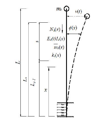
The model presented in Figure 1 represents a column fixed at the bottom and free at the top end, in undamped free vibration, approximating the mathematical model of the structural dynamics field to the practical problem proposed, using modal analysis, where t indicates time, ϕ(x) represents the shape function of the oscillatory motion, L is the total length (or height) of the structure, L _s and L _s−1 are the height at the upper and lower limits of a given segment s, whose length is obtained by the difference between these two positions, and v(t) is the generalized coordinate localized at the free extremity of the column. Equation (1) refers to a trigonometric function taken as a shape function, considered valid at any point in the structural domain and that obeys the boundary conditions of the problem:

$\varphi (x)=1-\cos \left(\frac{\pi x}{2L}\right),$ (1)

where x starts at the base. This model represents a column under axial compressive load N(x) that can have constant or variable properties along the length. These properties include the geometry, elasticity or viscoelasticity and density. Springs k _s(x) are applied to represent the lateral soil-structure interaction.

Figure 1
Mathematical model for stability analysis.

With these conditions, the column is under the influence of gravitational forces, originating from the distributed mass due to the self-weight of the structure and other added masses; and of a concentrated mass at the free top end, to be defined in the event of loss of stability, whose value represents the vertical maximum load that can be applied.

To get the analytical solution of this problem, it was necessary to consider a mathematical function to reduce the problem to a system with only one degree of freedom. For the present case, a trigonometric function given by Equation (1) was adopted. The use of Equation (1) as a valid shape function for a structure with variable geometry was validated by Wahrhaftig (2019a) in comparison to computational analyses using the finite-element method (FEM). The FEM is a technique to discretize the continuum that has been used recently in computer modeling to analyze buckling and vibration of reinforced concrete structures, as mentioned by Rodrigues et al. (2014), who studied concrete columns eccentrically loaded, considering nonlinearities inherent in the system, including creep and shrinkage, for sections with reinforcement ratio of 1.98% and 3.95%, by Bueno and Loriggio (2016), who evaluated undamped free vibrations of reinforced concrete decks in relation to recommended limit states, and also by Rajasekaran and Khaniki (2018), who assessed buckling of beams with functional graded materials.

Applying the principle of virtual work and its derivatives, similarly to that done by Clough and Penzien (1995), the dynamic properties of interest are obtained. The conventional elastic/viscoelastic stiffness is specified as:

$k_{0s}(t)={{\displaystyle {\int }_{L_{s-1}}^{L_s}{E}_s(t)I_s(x)\left(\frac{d^2\varphi (x)}{d{x}^2}\right)}}^{2}dx,$ (2)

with

$K_0(t)={\displaystyle \sum _{s=1}^n{k}_{0s}(t)},$ (3)

where, for the segment s of the structure, E _s(t) is the viscoelastic module of the material as a function of time, I _s(x) is the moment of inertia that varies along the segment about the considered motion, obtained by interpolation of subsequent sections, all homogenized (if constant, it is simply going to be I _s), k _0s(t) is the term for stiffness variation over time, K ₀(t) is the final stiffness varying with time, and n is the total number of segments in the analyzed geometry. If the material exclusively shows elastic behavior, the respective equations will not be functions of time anymore.

The geometric stiffness presents as a function of the axial force, including the self-weight contribution, being calculated as follows:

$k_{gs}(m_0)={\displaystyle \underset{L_{s-1}}{\overset{L_s}{\int }}\left[N_0(m_0)+{\displaystyle \sum _{j=s+1}^n{N}_j}+{\overline{m}}_s(x)(L_s-x)g\right]{\left(\frac{d\varphi (x)}{dx}\right)}^{2}dx},$ (4)

with “j” being just a counter for the summation,

$N_0(m_0)=m_{0}g,$ (5)

and

$K_g(m_0)={\displaystyle \sum _{s=1}^n{k}_{gs}(}{m}_0),$ (6)

where k _gs(m ₀) is the geometric stiffness of segment s, N ₀(m ₀) is the concentrated force at the top part of the system, calculated by Equation (5), and K _g(m ₀) is the total geometric stiffness of the structure, given by Equation (6); as can be seen, all of them depend on the mass m ₀ located at the free end of the structure. In Equation (4), N _s represents the normal force in the upper segments above the considered segment, which can be obtained from:

$N_s={\displaystyle \underset{L_{s-1}}{\overset{L_s}{\int }}{\overline{m}}_s}(x)gdx,$ (7)

where ${\overline{m}}_s(x)$ is the mass per unit length. Thereby, the generalized total mass is specified as:

$M(m_0)=m_0+m,$ (8)

considering:

$m={\displaystyle \sum _{s=1}^n{m}_s},$ (9)

with

$m_s={\displaystyle \underset{L_{s-1}}{\overset{L_s}{\int }}{\overline{m}}_s}(x){\left(\varphi (x)\right)}^{2}dx,$ (10)

and

${\overline{m}}_s(x)=A_s(x){\rho }_s,$ (11)

where A _s(x) represents the cross-section area and ρ _s is the material density for the respective segment s. If the cross-section has a constant area along the interval, A _s(x) will be A _s , and consequently the mass distribution per unit length will also be constant. In the same way, if the mass m ₀ does not vary, all of its dependent parameters will also be constant.

In order to consider the soil influence on the system vibration, it was necessary to consider it as a series of vertically distributed springs along the foundation that act to introduce a restoring force into the structural system. With k _s (x) denoting the spring parameter, the effective stiffness of the soil, as a function of the variable x along the length, can be defined as:

$K_{Soil}={\displaystyle \sum _{s=1}^n{k}_{soil}},$ (12)

with

$k_{soil}={\displaystyle \underset{L_{s-1}}{\overset{L_s}{\int }}{k}_s(x)\varphi {(x)}^{2}dx},$ (13)

and

$k_s(x)=S_s{D}_s(x),$ (14)

where the parameter k _Soil is an elastic property that consists of the sum of k _s (x) along the depth of the foundation, which depends on its geometry D _s (x) and on the elastic parameter of the soil S _s , considered constant, in this case, on each layer, although it may not necessarily be constant. Considering as positive a compressive normal force, it is possible to obtain the total stiffness of the system as a function with two variables:

$K(m_0,t)=K_0(t)-K_g(m_0)+K_{Soil}.$ (15)

Accordingly, the frequency can be calculated, in hertz, with Equation (16), as a function of time and concentrated mass at the free end.

$f(m_0,t)=\frac{1}{2\pi }\sqrt{\frac{K(m_0,t)}{M(m_0)}}.$ (16)

The mathematical method previously described defines the critical buckling load for the nullity of the frequency, representing the occasion at which the structure loses its stiffness. All generalized parameters, such as total stiffness, Equation (15), total mass, Equation (8), as well as the normal force at the free end, Equation (6), were expressed as a function of the concentrated mass at the top part. When the creep is introduced into the analysis, it will be necessary to consider a model that represent the viscoelastic behavior of concrete, and after that, the frequency becomes a time-dependent function, since the modulus of elasticity is also time-dependent. Thus, by writing the frequency in terms of time and concentrated mass at the free end, Equation (16), the critical buckling load is established for a determined value that makes the frequency becomes null, at any instant of interest, that multiplied by the gravitational acceleration, will define the force corresponding to the collapse of the system.

Taking all the previous considerations into account, and assuming the concentrated mass as an independent variable of the problem, the critical buckling load N _bk can be determined by using the mathematical concept in Equation (17), and the details of the present analytical process can be found in Wahrhaftig et al. (2019b).

$f(m_0,t)=0\Rightarrow N_0(m_0)=N_{bk}.$ (17)

3 CREEP CRITERIA ACCORDING TO THE BRAZILIAN CODE

The model proposed by NBR 6118:2014 (ABNT, 2014) considers the creep strain ε _cc to be composed by two terms, one related to the fast strain ε _cca and the other one to the slow strain ε _ccb . The fast strain is irreversible and happens during the first twenty-four hours after the structure is submitted to loading. On the other hand, the slow strain has two other parts, the slow irreversible strain ε _ccf and the slow reversible strain ε _ccd . Equation (18) shows the terms used in the determination of concrete creep and the slow strain,

${\epsilon }_{cc}={\epsilon }_{cca}+{\epsilon }_{ccf}+{\epsilon }_{ccd},$ (18)

and Equation (19) represents the total strain of concrete ε _c,tot which includes an immediate one ε _c .

${\epsilon }_{c,tot}={\epsilon }_c+{\epsilon }_{cc}.$ (19)

Since the slow strain of concrete ε _cc can be expressed in terms of the creep strain coefficient φ, Equation (19) can be replaced by Equation (20),

${\epsilon }_{c,tot}={\epsilon }_c(1+\phi ),$ (20)

in which the creep strain coefficient φ is decomposed into the fast strain φ _a , the slow irreversible strain φ _f , and the slow reversible strain φ _d , according to Equation (21),

$\phi ={\phi }_a+{\phi }_f+{\phi }_d.$ (21)

The fast strain is calculated by the ratio between the concrete strength at the time of the load application and its final strength. The slow irreversible strain is determined as a function of the relative humidity, concrete consistency at placing, assumed thickness of the member, and assumed age of the concrete at the moment of loading. The slow reversible strain depends only on the duration of loading. Its final value and development over time do not depend on the age of concrete at the instant of the load application.

NBR 6118:2014 (ABNT, 2014) introduces some hypotheses that are adopted to define the creep effects when the stresses in the concrete are related to normal service loads. The first one is the consideration of linear variation between the applied stress and the creep strain ε _cc . It is also considered that, for the same concrete, the strain curves of the irreversible slow strain φ _f as a function of time, and corresponding to different ages of the concrete at the moment of the loading, are obtained one in relation to each other by parallel dislocation of the strain axis, as shown in Figure 2.

Figure 2
Variation of the slow irreversible strain over time (ABNT-NBR 6118:2014).

NBR 6118:2014 (ABNT, 2014) preconizes that when the determination of the concrete creep is desired to be done for a certain instant t, Equation (18) can be written as a function of time, as can be seen in Equation (22), from which an also time-dependent function of the modulus of elasticity is originated, in terms of the creep coefficient φ(t,t ₀ ):

${\epsilon }_{cc}(t,t_0)={\epsilon }_{cca}+{\epsilon }_{ccf}+{\epsilon }_{ccd}=\frac{{\sigma }_c}{E_{c28}}\phi (t,t_0),$ (22)

where ε _cc (t,t ₀ ) represents the variation over time of the strain due to creep, σ _c is the stress in the concrete, E _c28 is the initial tangent modulus at twenty-eight days, and φ(t,t ₀ ) is the creep coefficient as a function of time, given by Equation (23):

$\phi (t,t_0)={\phi }_a(t,t_0)+{\phi }_{f\infty }[{\beta }_f(t)-{\beta }_f(t_0)]+{\phi }_{d\infty }{\beta }_d(t,t_0),$ (23)

where t is the assumed concrete age for the considered instant, in days; t ₀ is the assumed concrete age at the moment of loading, also in days, with φ _a calculated by Equation (24); the coefficient φ _f∞ is the final value for the slow strain given by Equation (25); β _f (t) and β _f (t ₀ ) are coefficients related to the slow irreversible strain, as a function of the age of the concrete obtained by Equation (26); φ _d∞ is the final value for the coefficient of the slow reversible strain that is considered equal to 0.4; and β _d is the coefficient related to the slow reversible strain, calculated as a function of time after loading (t - t ₀ ), expressed by Equation (27):

${\phi }_a=0.8\left[1-\frac{f_c(t_0)}{f_c(t_{\infty })}\right],$ (24)

${\phi }_{f\infty }={\phi }_{1c}{\phi }_{2c},$ (25)

${\beta }_f(t)=\frac{t^2+At+B}{t^2+Ct+D},$ (26)

${\beta }_d(t)=\frac{t-t_0+20}{t-t_0+70}.$ (27)

Note that the relation between f _c (t ₀ ) and f _c (t _∞ ) represents the strength gain curve of concrete; φ _1c is the coefficient that depends on the relative humidity, in percentage, and on the consistency of the concrete, and φ _2c is the coefficient depending on the assumed thickness of the member, defined by Equation (28); and the A, B, C and D terms are related to the coefficient for slow irreversible strain and can be calculated by the following Equations (29), (30), (31) and (32), respectively:

${\phi }_{2c}=\frac{42+h_{fic}}{20+h_{fic}},$ (28)

$A=42h^3-350h^2+588h+\mathrm{113,}$ (29)

$B=768h^3-3060h^2+3234h-\mathrm{23,}$ (30)

$C=-200h^3+13h^2+1090h+\mathrm{183,}$ (31)

$D=7579h^3-31916h^2+35343h+\mathrm{1931,}$ (32)

where h _fic and h denote the assumed thickness of the analyzed member, in centimeters and meters, respectively. Therefore, the time-dependent function referred to as the modulus of elasticity can be described by Equation (33):

$E(t,t_0)=\frac{1}{\frac{1}{E_{c0}}+\frac{\phi (t,t_0)}{E_{c28}}},$ (33)

where E _c0 is the modulus of elasticity of concrete at the instant of loading.

4 EVALUATION OF A CASE STUDY

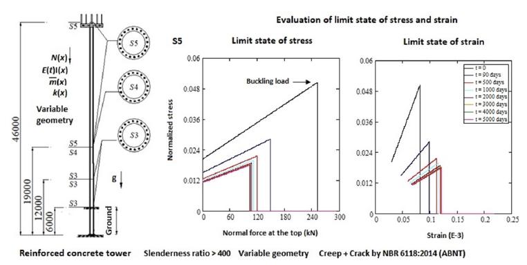
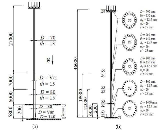
The analyzed structure in this evaluation is a real pole, extremely slender, made from reinforced concrete, with variable geometry, shown in Figure 3, that is 46 m high, including a 40 m superstructure, with hollow circular cross-section, and the 6 m deep foundation, which is relatively deep, is a belled shaft foundation. The dimensions, heights and structural arrangement of the column and column segments are shown in Figure 4, (a) and (b), where g is the gravitational acceleration; S1, S2, S3, S4, and S5 are the cross-sections; D and th indicate the external diameter and wall thickness, respectively; d _b represents the diameter of steel bars; n _b is the number of bars, c´ is the cover of concrete in the respective cross-sections, and “Var” indicates tapered section at the segment.

Figure 3
Pictures of the reinforced concrete pole

Figure 4
Details of geometry (a), heights and structural arrangement (b).

It is worth mentioning that, although the average wall thickness of the cross-sections represents 0.72% of the height of the superstructure, no analyses regarding the local buckling or distortion of the section were considered, since it is a problem that should be treated with another specific approach, as discussed by Pierin and Silva (2015). Therefore, the present approximation is restricted to the global instability evaluation, similar to the work developed by Schnabl and Planinc (2017). The moduli of elasticity of concrete at 28 days for the superstructure and foundation, solved with Equation (34) and (35), with f _ck in MPa for both Equations, are, respectively, 34278.92 MPa and 21287.37 MPa, considering nominal strengths f _ck equal to 45 MPa and 20 MPa:

$E_{c28}={\alpha }_i\cdot 5600\sqrt{f_{ck}},where{\alpha }_{i}isfoundby$ (34)

${\alpha }_i\text{}=0.8+0.2\cdot \frac{f_{ck}}{80MPa}.$ (35)

Usually, equipment is attached at the top of the structure, settling a concentrated mass applied at the free end of the column, in which the limit value in relation to the stability loss due to buckling should be determined. Additional devices are also installed along all the structure, adding a distributed mass of 40 kg/m.

The foundation is a belled shaft, with a bell diameter of 140 cm and length of 20 cm; the shaft is 80 cm in diameter and 580 cm long. The lateral soil pressure was represented by an elastic parameter equal to 2669 kN/m³. The physical nonlinearity of the RC was computed following the recommendations from NBR 6118:2014 (ABNT, 2014), which suggests a 50% reduction in the section moment of inertia for analyses under similar circumstances, regardless of the possibility to choose another reduction factor, as discussed by Marin and El Debs (2012), but also considering the fact that columns in buildings normally have the same cross-section between floors. The density of reinforced concrete was assumed to be 2600 kg/m³ for the superstructure and 2500 kg/m³ for the foundation.

To take the steel bars into consideration in the calculation of the cross-section moment of inertia, homogenization factors were used, multiplying the nominal moment of inertia in each section. Using the parallel axis theorem, the values were found to be 1.026, 1.074, 1.050, 1.061, and 1.064 for the sections 1 to 5, respectively, at the commence of loading. The creep due to the viscoelastic behavior of concrete was accounted for in the structure as recommended by NBR 6118:2014 (ABNT, 2014). Studies regarding creep effects transferred to the steel in reinforced concrete columns can be found in Kataoka and Bittencourt (2014) and Madureira et al. (2013). Despite the description of the stress transfer to reinforcement steel in the study by Kataoka and Bittencourt (2014), made with short specimens, the numerical evaluation was found to be inconclusive in the study. In their first work, Madureira et al. (2013) describe the transfer mechanism in which forces are carried to the reinforcement steel due to creep of concrete and also indicate that there may be a convergence of the strains after 3000 days of loading. In a second investigation, Madureira and Paiva (2018) discuss the stress transfer to the reinforcement steel due to the creep of concrete in bent RC members.

5 RESULTS AND DISCUSSION

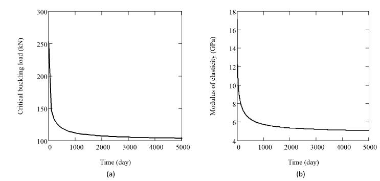
The variation of the critical buckling load and modulus of elasticity over time, as summarized by Equations (17) and (33), can be seen in the graphs in Figure 5, (a) and (b), respectively. The latter provides important information for temporary loading and construction with time of use less than one of the mentioned moments. In order to calculate the variation of the critical load over time, a small computer program was developed, considering a mass increment of 0.1 kg, a time frame of 100 days, and a frequency with 10⁻³ Hz precision.

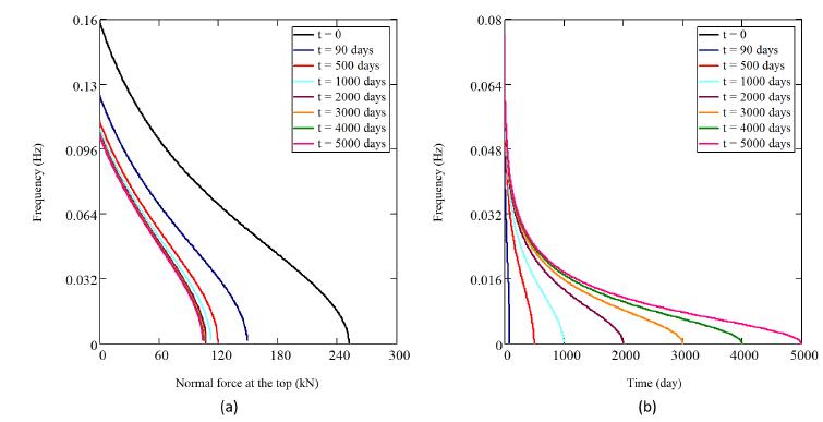
Besides the arbitrarily chosen intervals, the analysis could be done for any other preferred period of time during the structure’s lifespan, although it is possible to notice that the convergence tends to occur after 5000 days from the beginning of the structure performance, as can be observed in Figure 6(a). Setting the normal force as the same value of the critical load, Figure 6(b) allows the assessment of the variation of the structural frequency over the period considered. The strain analysis in the ultimate limit state (ULS) of a compressed element can be executed by examining the graphs in Figure 7, where it is possible to verify that, at the instants of time defined for the evaluation, the strains are below the limit of 0.002 (0.20%) set by NBR 6118:14 (ABNT, 2014), the value that denotes when the cracks start to occur in the concrete in compression (Tamayo et al.,2015). The maximum strain value found under the critical buckling load at the most unfavorable instant was 0.12‰, which represents 6.07% of the limit previously set.

Figure 5
Variation over time of: (a) critical buckling load; (b) modulus of elasticity.

Figure 6
Structural frequency: (a) with force at the top; (b) over time for critical buckling load.

These results were obtained by taking into account the total strain of the structure and by computing the strength gain of the concrete as well as the homogenization of the sections, given by Equations (36), (37) and (39). Equation 36 is modified from the original equation proposed in the Eurocode (EN 1992-1-1:2004) to estimate the compressive strength of concrete at various ages, introducing the factor of safety γ _c , equal to 1.4, according NBR 6118:2014 (ABNT, 2014).

$f_c(t)={\beta }_1\frac{f_{ck}}{{\gamma }_c},$ (36)

and

${\beta }_1(t)=e^{0.38\left(1-\sqrt{\frac{28day}{t}}\right)},$ (37)

with t in day.

Figure 7
Analysis of the limit state for axial strain.

The results presented in Figure 7 are compatible with the findings of Fischer et al. (2014), who experimentally analyzed standard specimens of concrete and verified the existence a linear response of creep to strain below 0.4. The relative stresses, expressed by the ratio between the induced stress in the homogenized section and the strength of concrete, as a function of the force at the top of the structure, can be seen in the graphs on the left in Figure 8, revealing results less than a unit. In fact, the relative stresses decrease over time due to force transfer to the reinforcement steel, influenced by the increase in the area homogenization factor, Equation (40), whose development is presented on the right side in Figure 8. When the normal force at the top equals the critical buckling load, the values found for the relative stresses in sections 3 to 5 were 4.91%, 5.18%, and 5.07%, respectively.

Figure 8
Relative stresses and homogenization factors in the concrete section

It is important to assess the reduced normal forces ((t) at the cross-sections of the structure when the force at the column free-end approaches the value of the critical buckling load, at the respective chosen instants of time. In order to do that, both the homogenization of the section as well as the strength gain of concrete over time were taken into account, using Equation (38),

$\eta (t)=\frac{N_{bk}(t)}{A_{\mathrm{hom}}(t)f_c(t)},$ (38)

where f _c (t) is the strength of concrete, given by Equation (36), and A _hom (t) is the homogenization of the concrete area, obtained by Equation (39)

$A_{\mathrm{hom}}(t)=A_{cn}+A_{st}\cdot \zeta (t),$ (39)

with

$\zeta (t)=\frac{E_{st}}{E(t)},$ (40)

in which A _cn is the net area of concrete, and A _st and E _st are the area of steel and the steel modulus of elasticity, respectively. With the decrease in the concrete modulus of elasticity, and consequent increase in the homogenization factor of the sections ζ(t), it is possible to verify that the internal forces, calculated by equilibrium of forces and compatibility of displacements, occur for an additional part of the loading taken by the reinforcement, compensating for the increase in strain due to creep, an effect that increases together with the reinforcement ratio.

Table 1 summarizes the obtained results, in which the reinforcement ratios (w) for the sections 3 to 5 are presented. The following considerations were made in the analyses of this paper: modulus of elasticity of reinforcement steel equal to 205 GPa, concrete production under standard conditions, relative humidity of 70%, and gravitational acceleration of 9.807 m/s².

Table 1
Obtained results.

t	E	ΔE	Nbk	Δ Nbk	m0	( (%)
(day)	(MPa)	(%)	(kN)	(%)	(kg)	S3 (w = 0.83%)	S4 (w = 0.99%)	S5 (w = 1.10%)
0	34278.92	-	252.239	-	25721.22	2.35	2.73	3.01
90	17516.54	48.9	149.451	40.75	15239.76	1.05	1.21	1.32
500	12680.81	27.61	119.799	19.84	12216.1	0.72	0.82	0.89
1000	11501.91	9.3	112.571	6.03	11479.05	0.65	0.73	0.80
2000	10736.11	6.66	107.874	4.17	11000.09	0.60	0.68	0.73
3000	10441.38	2.75	106.067	1.68	10815.82	0.58	0.66	0.71
4000	10284.57	1.5	105.106	0.91	10717.83	0.57	0.65	0.70
5000	10187.00	0.95	104.508	0.57	10656.85	0.56	0.64	0.69
Variation	70.28%	-	58.57%	-	58.57%	-	-	-

• E = modulus of elasticity; Δ = variation at the subsequent instant; N bk = buckling load; m 0 = mass at the free end; ( = reduced normal force; w = reinforcement ratio; S3, S4, S5 are cross-sections 3, 4, 5.

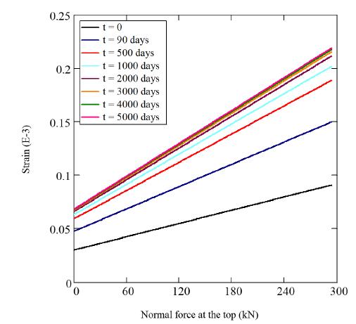
Setting the buckling load as the loading limit that can be applied to each section, with σ(m ₀ ) as the stress acting in the section as a function of the normal top force and σ _u(t) = N _bk (t)/A _hom (t), the normalized stress σ(m ₀ )/σ _u(t) becomes a bilinear function composed of inclined and vertical segments, as shown in Figure 9, where the curve’s inflection point at each instant corresponds to the critical buckling load (CBL), from which the structure finds itself on the verge of collapse and any minimal load no longer can be applied. The decreasing of the normalized stress with the time rises with the increasing of the homogenized area of concrete, due the growing of ζ(t) in Equation (40). That means the creep decreases the stress on the sections in terms of the ULS (ultimate limit state) of the capacity resistance under vertical force, Figure 9(left), even though it lifts the strain of the structure, Figure 9(right). In the latter aspect, it is possible to see that the self-weight of the structure imposes an initial strain on the system, and strains are not starting from zero even with no single lumped mass applied.

Figure 9
Normalized stress on the homogenized concrete section in ULS (CBL = Critical buckling load).

As a result of the concrete creep, there is an axial stress transfer from the concrete to the reinforcing bars, without reaching the yield stress of steel, though. In fact, as displayed in Figure 10, the stress in the reinforcement shows a linear growth, reaching the maximum value at the critical buckling load. Calculations that include the weight of upper segments led to the following results: stress of 37.47 MPa (7.49% of f _y ) at the critical load for section S3; 42.40 MPa (8.48% of f _y ) for section S4; and 30.91 MPa (6.18% of f _y ) for section S5, all with steel yield strength f _y = 500 MPa. Obviously, the interpretation of these graphs implies understanding their validity until the critical buckling load. Even when admitting a large spectrum of values of the normal force at the top, that overcome the limit value stresses, the reinforcement steel remains in the elastic zone and much below to yield.

Figure 10
Stresses in the reinforced area

5 CONCLUSIONS

The critical buckling load for a real reinforced concrete structure has been determined using an analytical method based on vibration concepts for structural systems. The analyzed structure presented geometric variations along its height, and all necessary parameters for calculations of the dynamics were considered, such as: geometric imperfections, considered by the geometric stiffness; the physical nonlinearity and creep of concrete, that were taken into account according to the recommendations from NBR 6118:2014 by ABNT.

Using the previous considerations in the analytical procedure, an axial compressive force of 252.24 kN at the initial instant and 104.51 kN after 5000 days from the beginning of the structure performance were defined for the buckling of the structure, with both values corresponding to a null first natural vibration frequency, which represents a 59% reduction in the structure’s vertical strength. Even with this reduction, the maximum buckling load the structure can withstand is higher than the loading usually applied to this kind of system. Important to note that no one factor of safety was assigned to the applied normal forces. It is important to clarify that according NBR 6118:2014 (ABNT, 2014) application of a safety coefficient of 1.4 for dead load is waited, being also necessary performing a verification for local second order effects when the slenderness ratio of a structural element is higher than 200.

Due to the creep, the modulus of elasticity exhibited a 70% variation during the considered time frame. The evaluation of induced stresses in the homogenized concrete section revealed a maximum percentage of 5.2% among those presented by different critical buckling loads. For the reinforcement, the maximum relative value found for the stress in the steel, with load transfer due to creep, was 8.5% of the material yield stress (500 MPa), ruling out the possibility of the steel to yield. The strain calculated at the most unfavorable conditions exhibited only 6.1% of the recommended limit. With these results, it has been proved that the critical buckling load determines not only the ultimate limit state to the loss of stability as a deformable solid but also the ultimate limit state for stress and stain for slender structures.

Lastly, it should be noted that the analytical method presented in this paper is free from the application of iterative methods or discretization processes, with a solution directly obtained in the continuum. This method may be adapted to include different geometries, with no, one or some concentrated masses (and forces) along the height, and, still, making it able to solve any problem that may be modeled as unidimensional elements, including buildings.

A comparative analysis between other calculation methods and design criteria from different design codes should be included in future studies, as well as the influences of mechanical and thermal-related strains, and also the consideration of other boundary conditions.

References

• Associação Brasileira de Normas Técnicas (2014). NBR 6118: Projeto de Estruturas de Concreto - Procedimento. Rio de Janeiro, 2014.
• Babu, R. R.; Benipal, G. S.; Singh, A. K., (2006). Plasticity-based constitutive model for concrete in stress space. Lat. Am. J. Solids Struct. 3: 417-441.
• Bueno, J. R.; Loriggio, D. D., (2016). Influence of the flexibility of beams and slabs in static response and dynamic properties. Rev. IBRACON Estrut. Mater. 9(6): 842-855. DOI:10.1590/s1983-41952016000600003.
  » https://doi.org/10.1590/s1983-41952016000600003
• Clough, R. W.; Penzien, J., (1995). Dynamics of Structures. Computers & Structures, Inc., Berkeley.
• European Committee for Standardization (2004). EN 1992-1-1 - Eurocode 2: Design of concrete structures - Part 1: General rules and rules for buildings. Brussels, 2004.
• Fischer, I.; Pichler, B.; Lach, E.; Terner, C., Barraud, E.; Britz, F., (2014). Compressive strength of cement paste as a function of loading rate: Experiments and engineering mechanics analysis. Cem. Concr. Res. 58: 186-200. DOI:10.1016/j.cemconres.2014.01.013.
  » https://doi.org/10.1016/j.cemconres.2014.01.013
• Geiker, M. R.; Michel, A.; Stang, H.; Lepech, M. D., (2019). Limit states for sustainable reinforced concrete structures. Cement Concrete Res. 112: 189-195. DOI:10.1016/j.cemconres.2019.04.013
  » https://doi.org/10.1016/j.cemconres.2019.04.013
• Greenhill, A. G., (1881). Determination of the greatest height consistent with stability that a vertical pole or mast can be made, and the greatest height to which a tree of given proportions can grow. Proc. Cambridge Philos. Soc. 4: 65-73.
• Kataoka L. T.; Bittencourt T. N., (2014). Numerical and experimental analysis of time-dependent load transfer in reinforced concrete columns. Rev. IBRACON Estrut. Mater. 7(5): 747-774. DOI:10.1590/S1983-41952014000500003.
  » https://doi.org/10.1590/S1983-41952014000500003
• Leitão, F. F.; Siqueira, G. H.; Vieira Jr., L. C. M.; Almeida, S. J. C., (2019). Analysis of the global second-order effects on irregular reinforced concrete structures using the natural period of vibration. Rev. IBRACON Estrut. Mater. 12(2): 408-428. DOI:10.1590/s1983-41952019000200012.
  » https://doi.org/10.1590/s1983-41952019000200012
• Madureira, E. L.; Paiva, L. A., (2018). Fresh concrete consistency effect on thin-walled columns creep phenomenon. Rev. IBRACON Estrut. Mater. 11(3): 644-651. DOI:10.1590/s1983-41952018000300012.
  » https://doi.org/10.1590/s1983-41952018000300012
• Madureira, E. L.; Siqueira, T. M.; Rodrigues, E. C., (2013). Creep strains on reinforced concrete columns. Rev. IBRACON Estrut. Mater. 6(4): 537-560. DOI:10.1590/S1983-41952013000400003.
  » https://doi.org/10.1590/S1983-41952013000400003
• Marin, M. C.; El Debs, M. K., (2012). Contribution to assessing the stiffness reduction of structural elements in the global stability analysis of precast concrete multi-storey buildings. Rev. IBRACON Estrut. Mater. 5(3): 316-342. DOI:10.1590/S1983-41952012000300005.
  » https://doi.org/10.1590/S1983-41952012000300005
• Metha, P. K.; Monteiro, P. J. M, Filho, A. C., (1994). Concreto: estrutura, propriedades e materiais. Ed. PINI, São Paulo, Brasil.
• NBR 6118:2014 Design of structural concrete - procedure. (2014). Brazilian Association for Standardization (ABNT). Rio de Janeiro, Brazil.
• Pierin, I.; Silva, V. P., (2015). Distortional buckling resistance of cold-formed steel. J. Braz. Soc. Mech. Sci. Eng. 37: 1163-1171. DOI:10.1007/s40430-014-0252-x.
  » https://doi.org/10.1007/s40430-014-0252-x
• Rajasekaran, S.; Khaniki, H. B., (2018). Bending, buckling and vibration analysis of functionally graded non-uniform nanobeams via finite element method. J. Braz. Soc. Mech. Sci. Eng. 40: 549. DOI:10.1007/s40430-018-1460-6.
  » https://doi.org/10.1007/s40430-018-1460-6
• Rayleigh (1877). Theory of sound. Dover Publications, New York. Reissued in 1945.
• Reis, D. G. ; Siqueira, G. H. ; Vieira Jr, L. C. M. ; Ziemian, R. D. (2018). Simplified Approach Based on the Natural Period of Vibration for Considering Second-Order Effects on Reinforced Concrete Frames. International Journal of Structural Stability and Dynamics. 18 (05): 1850074-1-1850074-20. DOI: 10.1142/S0219455418500748
  » https://doi.org/10.1142/S0219455418500748
• Rodrigues, E.A.; Manzoli, O.L.; Bitencourt Jr, L.A.G.; Prazeres, P.G.C.; Bittencourt, T.N., (2014). Failure behavior modeling of slender reinforced concrete columns subjected to eccentric load. Lat. Am. J Solids Struct. 12: 520-541. DOI:10.1590/1679-78251224.
  » https://doi.org/10.1590/1679-78251224
• Rosa, L. M. P.; Danziger, B. R.; Carvalho, E. M. L., (2018). Soil-structure interaction analysis considering concrete creep and shrinkage. Rev. IBRACON Estrut. Mater. 11(3): 564-585. DOI:10.1590/s1983-41952018000300008.
  » https://doi.org/10.1590/s1983-41952018000300008
• Schnabl, S.; Planinc, I., (2017). Buckling of slender concrete-filled steel tubes with compliant interfaces. Lat. Am. J. Solids Struct. 14(10): 1837-1852. DOI:10.1590/1679-78253479.
  » https://doi.org/10.1590/1679-78253479
• Shaikh, F. U. A., (2018). Effect of cracking on corrosion of steel in concrete. Int. J. Concr. Struct. Mater 12: 3. DOI:10.1186/s40069-018-0234-y.
  » https://doi.org/10.1186/s40069-018-0234-y
• Shiki, S. B.; Lopes Jr., V.; da Silva, S., (2014). Identification of nonlinear structures using discrete-time Volterra series. J. Braz. Soc. Mech. Sci. Eng., 36(3): 523-532. DOI:10.1007/s40430-013-0088-9.
  » https://doi.org/10.1007/s40430-013-0088-9
• Suter, M.; Benipal, G. S., (2007). Time-dependent behaviour of reacting viscoelastic concrete. Lat. Am. J. Solids Struct. 4(2): 103-120.
• Tamayo, J.L.P.; Morsch, I.B.; Awruch, A.M., (2015). Short-time numerical analysis of steel-concrete composite beams. J. Braz. Soc. Mech. Sci. Eng. 37(4): 1097-1109. DOI:10.1007/s40430-014-0237-9.
  » https://doi.org/10.1007/s40430-014-0237-9
• Timoshenko, S. P.; Gere, J. M., (1961). Theory of elastic stability, 2nd ed. McGraw-Hill Book Company, New York.
• Wahrhaftig, A. M., (2019a). Analysis of the first modal shape using two case studies. Int. J. Comput. Meth. 16(6): 1840019. DOI:10.1142/S0219876218400194.
  » https://doi.org/10.1142/S0219876218400194
• Wahrhaftig, A. M.; Brasil, R. M. L. R. F., (2016). Vibration analysis of mobile phone mast system by Rayleigh method. Appl. Math. Modell. 42: 330-345. DOI:10.1016/j.apm.2016.10.020.
  » https://doi.org/10.1016/j.apm.2016.10.020
• Wahrhaftig, A. M.; Brasil, R. M. L. R. F., (2017). Initial undamped resonant frequency of slender structures considering nonlinear geometric effects: the case of a 60.8 m-high mobile phone mast. J. Braz. Soc. Mech. Sci. Eng. 39(3): 725-735. DOI:10.1007/s40430-016-0547-1.
  » https://doi.org/10.1007/s40430-016-0547-1
• Wahrhaftig, A. M.; Brasil, R. M. L. R. F.; Balthazar, J. M., (2013). The first frequency of cantilever bars with geometric effect: a mathematical and experimental evaluation. J. Braz. Soc. Mech. Sci. Eng.; 35(4): 457-467. DOI:10.1007/s40430-013-0043-9.
  » https://doi.org/10.1007/s40430-013-0043-9
• Wahrhaftig, A. M.; Silva, M. A.; Brasil, R. M. L. R. F., (2019b). Analytical determination of the vibration frequencies and buckling loads of slender reinforced concrete towers. Lat. Am. J. Solids Struct. 16(5): e196. DOI:10.1590/1679-78255374.
  » https://doi.org/10.1590/1679-78255374
• Yazdchi, M.; Khalili, N.; Valliappan, S., (1999). Dynamic soil-structure interaction analysis via coupled finite-element-boundary-element method. Soil. Dyn. Earthq. Eng. 18(7): 499-517. DOI:10.1016/S0267-7261(99)00019-6.
  » https://doi.org/10.1016/S0267-7261(99)00019-6
• Zaman, M.; Desai, C. S.; Drumm, E. C., (1984). Interface model for dynamic soil-structure interaction. J. Geotech. Geoenviron. 110(9): 1257-1273. DOI:10.1061/(ASCE)0733-9410(1984)110:9(1257).
  » https://doi.org/10.1061/(ASCE)0733-9410(1984)110:9(1257)

Edited by

Editor:

Pablo Andrés Muñoz Rojas.

Publication Dates

• Publication in this collection
  03 Feb 2020
• Date of issue
  2020

History

• Received
  29 Aug 2019
• Reviewed
  22 Nov 2019
• Accepted
  17 Dec 2019
• Published
  07 Jan 2020