From regional to local scale modelling on the south-eastern Brazilian shelf: case study of Paranaguá estuarine system

Abstract

The applicability of a numerical model following a downscaling methodology was evaluated for the south-eastern Brazilian shelf (regional model) and Paranaguá estuarine system (local model). This approach permits the simulation of different scale processes, such as storm surges and coastal upwelling, and is suitable for operational forecasting purposes. When large areas are covered by regional models, the tidal propagation inside the domain can be significantly affected by the local tidal potential, mainly where the resonance phenomenon is observed. The south-eastern Brazilian shelf is known for the resonance of the third-diurnal principal lunar tidal constituent (M3), the largest amplitudes being found in the Paranaguá estuarine system. Therefore, the significance of the local tidal potential was assessed in this study for the most important tidal constituents inside the estuarine system (including M3). The model validation was performed with tidal gauge data, Argo float profiles and satellite measurements of Sea Surface Temperature. The methodology described in this study can be replicated for other important estuarine systems located on the south-eastern Brazilian shelf. Furthermore, the numerical model was developed within a perspective of operational nowcast/forecast simulations, useful for several activities such as navigation and response to emergencies (e.g., oil spills).

Descriptors:
Numerical modelling; Tidal propagation; Resonance phenomenon; Downscaling; South-eastern Brazilian shelf; Paranaguá estuarine system

Resumo

A aplicabilidade de um modelo numérico seguindo uma metodologia de downscaling foi avaliada para a plataforma sudeste brasileira (modelo regional) e o sistema estuarino de Paranaguá (modelo local). Esta abordagem permite simular fenômenos de escalas diferentes, como maré meteorológica e ressurgência costeira, e é apropriada para fins de previsão operacional. Quando grandes áreas são cobertas por modelos regionais, a propagação da maré no interior do domínio pode ser afetada significativamente pelo potencial local da maré, principalmente onde o fenômeno de ressonância é observado. A plataforma sudeste brasileira é conhecida pela ressonância da constituinte da maré lunar principal terci-diurna (M3), com as maiores amplitudes encontradas no sistema estuarino de Paranaguá. Por este motivo, a significância do potencial local da maré foi verificada neste estudo para as constituintes da maré mais importantes dentro do sistema estuarino (incluindo a M3). A validação do modelo foi realizada com dados de marégrafos, perfis de boias Argo e medições de satélite da temperatura da superfície do mar. A metodologia descrita neste estudo pode ser replicada para outros sistemas estuarinos importantes localizados na plataforma sudeste brasileira. Além disso, o modelo numérico foi desenvolvido na perspectiva de simulações operacionais em nowcast/forecast, úteis para diversas atividades, como navegação e resposta a emergências (e.g., derrames de petróleo).

Descritores:
Modelagem numérica; Propagação da maré; Fenômeno de ressonância; Downscaling; Plataforma sudeste brasileira; Sistema estuarino de Paranaguá

INTRODUCTION

Coastal circulation is governed by a variety of processes on different temporal and spatial scales, including tidal motion, wind action, oceanic currents, density stratification, internal waves and fresh water discharges. These processes are affected by coastline geometry and shelf topographic features. Particularly on broad shelves, tidal motion is amplified and the response to wind action is more intense (KANTHA; CLAYSON, 2000). Typically, depths at the shelf break are about 200 m, decreasing shoreward, while the shelf width varies between tens and hundreds of kilometres. The bottom friction in shallow depths is important in generating overtides and compound tides (PARKER, 1991). When the shelf width is about one-quarter of the tidal wavelength, the phenomenon of resonance amplifies the tidal ranges (HUTHNANCE, 1980).

The great complexity of coastal circulation can be better understood by the application of numerical models. Regional and local models can be nested to simulate processes on different spatial scales, such as storm surges generated mainly by wind action over thousands of kilometres, or the friction and influence of the coastline on the flow, which need higher resolution numerical grids to be properly solved. Moreover, the computational domain should include both the continental shelf and continental slope to simulate coastal upwelling. This process is one of the main mechanisms behind the nutrient availability in the mixed layer, controlling phytoplankton growth. The downscaling approach was previously applied in the Tagus estuary (Portugal) to study cohesive sediment dynamics (FRANZ et al., 2014a) and for operational modelling of hydrodynamics and water quality (FRANZ et al., 2014b). From the point of view of an operational forecast system, a downscaling from regional to local models has proven successful (e.g. MARALDI et al., 2013; BRICHENO et al., 2014; MATEUS et al., 2012).

The tidal forcing in regional models is usually given from a global tidal atlas, defining amplitudes and phases of tidal constituents at the open boundaries, which are converted into tidal levels. However, regional models usually cover a large area, thus making it important to include the local tidal potential, mainly when the resonance phenomenon is observed (WIJERATNE et al., 2012). The local potential interacts with the open boundary tidal forcing, amplifying or attenuating the tidal constituents, depending on the relative phases (ODAMAKI, 1989; CUMMINS et al., 2010; GOUILLON et al., 2010).

The south-eastern Brazilian shelf is known for the resonance of the third-diurnal principal lunar tidal constituent (M3), with the largest amplitudes found in the Paranaguá estuarine system. HUTHNANCE (1980) was the first to investigate this phenomenon with a semi-analytical model, reinforcing the theory of a damped 'organ-pipe' quarter wave resonance between the coast and the shelf edge. M3 is generated by the third-degree term in the lunar tidal potential, with a period of 8.28 h (KANTHA; CLAYSON, 2000). Due to its usually small amplitudes, M3 is often neglected in numerical modelling studies. Nevertheless, on the south-eastern Brazilian shelf, particularly in the Paranaguá estuary, M3 is one of the most important tidal constituents.

The main purpose of this paper is to evaluate the methodology of downscaling with nested models for the south-eastern Brazilian shelf (regional model) and the Paranaguá estuarine system (local model). A novelty of this study is the inclusion of M3 in the local tidal potential. To our knowledge, this is the first attempt to implement a numerical model for the Paranaguá estuarine system on the basis of a downscaling from a regional model. This approach allows the definition of realistic values of current velocities and water levels as boundary conditions, taking the effect of storm surges into consideration. When the effect of density on circulation is included (baroclinic mode), realistic values of temperature and salinity can be provided by the regional model, which is able to represent coastal upwelling.

The model was validated with tidal gauges and the significance of the local tidal potential was assessed for the most important tidal constituents, including M3. The importance of bottom friction and grid resolution for tidal propagation along the local model was also investigated. Salinity and temperature results were validated in the regional model domain with float profiles and Sea Surface Temperature from satellite measurements, verifying the capability to properly provide open boundary conditions for the local model.

This paper is divided into six sections. A brief description of the study area is given in Section 2, followed by a summary of relevant previous studies (Section 3). The methodology is described in Section 4, addressing the numerical model used, giving a definition of model domains and the numerical simulations performed. In Section 5 is presented a harmonic analysis of the tidal gauge data collected to characterize the tidal propagation inside the Paranaguá estuarine system, beyond the results of the numerical simulations. A discussion of the study's findings is presented in Section 6.

Study Area

The geometry features of the south-eastern Brazilian shelf and Paranaguá estuarine system are presented in Figure 1. This estuarine system has a surface area of 552 km² (excluding wetlands), 25% of which corresponds to a tidal flat region. The wetlands (mangrove areas and salt marshes) around the system cover an area of 296 km² (NOERNBERG et al., 2006). It is interconnected to the Cananéia-Iguape estuarine system by a narrow channel. Three inlet channels connect the Paranaguá estuarine system directly to the shelf sea. The two main channels are located around an Island (Ilha do Mel) at the system's mouth. These channels follow different predominant directions in the two main branches. A narrower branch lies in the east-west direction (Paranaguá bay), with an extension of about 40 km from the mouth. A broader branch lies in the north-south direction (Laranjeiras bay), with an extension of about 30 km from the mouth. The third and least important inlet channel is between two islands (Ilha das Peças and Ilha de Superagüi), connected to the central part of Laranjeiras bay.

Figure 1
Geometry features of the south-eastern Brazilian shelf (right) and Paranaguá estuarine system (left) with wetlands, showing the tidal gauges sites used for model validation.

The wind over the south-eastern Brazilian shelf is driven by the South Atlantic Convergence Zone (SACZ), with predominantly north-easterly winds, especially in summer. During the winter, the passages of cold fronts are more frequent, significantly changing the wind direction. The circulation at the shelf edge is dominated by the Brazil current (southward), leading to a strong eddy activity on the south-eastern Brazilian shelf. The Brazil current also induces shelf break upwelling, which is reinforced by wind driven upwelling in the summer (CAMPOS et al., 1995; CAMPOS et al., 2000). Furthermore, internal waves are generated over the shelf break and slope (PEREIRA; CASTRO, 2007a; PEREIRA et al., 2007b).

Previous studies

In the late 1970s, oceanographic and meteorological data on the south-eastern Brazilian shelf were measured by the University of São Paulo. The water level and currents at three sites on the shelf (PPR, PST and PRJ, in Figure 1) were used to define amplitudes, phases and current ellipses of the nine most important tidal constituents (Q1, O1, P1, K1, N2, M2, S2, K2, M3), as described by MESQUITA and HARARI (2003). The extension of the water level record used in the harmonic analysis varied between 12.9 and 31.2 days, with sampling intervals of 15 minutes. HARARI and CAMARGO (1994) used these amplitudes and phases to determine, through linear interpolation, the boundary conditions for a coastal hydrodynamic numerical model (three-dimensional, but barotropic). Following this approach, they were able to draw co-tidal charts and surface current ellipses for the main tidal constituents.

In another study, CAMARGO and HARARI (1994) considered wind and pressure fields in the same model to address storm surges in extreme events. At the open boundary, the water level oscillations caused by storm surges were defined proportionally to corresponding observations on coastal tidal gauges. Although this approach has led to satisfactory results in hindcast simulations, it is impracticable in operational modelling systems that are intended to produce forecasts. Furthermore, the model's results showed constraints in the representation of tidal amplitude and phase in the southern part of the shelf, mainly in neap tides and in the mouth of the Paranaguá estuarine system. The three high and low tides observed daily in neap tides were not properly represented by the model. This fact was explained as being due to the lack of non-linear tidal constituents in the model.

CAMARGO and HARARI (2003) used the cotidal amplitude and phase maps of HARARI and CAMARGO (1994) to implement a three-dimensional hydrodynamic model with a horizontal resolution of about 1 km for the Paranaguá estuarine system and neighboring coast, taking three non-linear tidal constituents into consideration in the simulations (M4, MN4, MS4). Due to the small area covered, the model only reproduced 10 % of the storm surge observed. This constraint can be overcome by coupling the local model to a larger scale model, which is one of the justifications for adopting a downscaling approach.

MATERIAL AND METHODS

Numerical Model

This study was based on the application of the MOHID water modelling system (LEITÃO et al., 2008). The hydrodynamic module is the core of MOHID. It is a three-dimensional model that solves the full Navier-Stokes equations, on the basis of the Boussinesq and hydrostatic approximations. The equations are solved numerically using the finite volumes method, with a generic vertical discretization that allows simultaneous implementation of various types of vertical coordinates. MOHID is coupled to GOTM (Global Ocean Turbulence Model), which consists of a set of turbulence-closure models (BUCHARD et al., 1999; VILLARREAL et al., 2005).

The open boundary tidal forcing for the hydrodynamic model was defined from FES2012 (Finite Element Solution) tidal atlas (LEFÈVRE et al., 2002; LYARD et al., 2006; CARRÈRE et al., 2012), which includes 32 tidal constituents distributed on 1/16º grids (amplitude and phase). Other smaller constituents were considered by tidal admittance. The choice of FES2012 was mainly based on the inclusion of the M3 tidal constituent. Furthermore, FES2012 has a better resolution and several more non-linear constituents than the previous version FES2004, which is a great improvement for coastal areas. Normally, the compound tides generated by non-linear effects in shallow waters are rapidly dissipated. A well-known exception is the M4 propagation from the Patagonian shelf towards the Brazilian coast (PAIRAUD et al., 2008). The tide was propagated into the nested domains using the Flather (1976) radiation scheme, which radiates external gravitational waves over the perturbation produced by other forcing mechanisms, such as wind and the Coriolis force.

The local tidal potential was included as a force added to the momentum equation. This local forcing interacts with the tidal propagation from the open boundary, which can amplify or attenuate the tidal constituents' amplitude and change their phase (GOUILLON et al., 2010). In shelf seas where resonance occurs, as observed on the south-eastern Brazilian shelf for the M3 tidal constituent, the local tidal potential can greatly affect the tide (WIJERATNE et al., 2012). MOHID was developed to take into account the second degree tidal potential for the most important long period (Mf, Mm, Ssa), diurnal (K1, O1, P1, Q1) and semidiurnal (M2, S2, N2, K2) tidal constituents, following the method described by KANTHA and CLAYSON (2000). The third degree tidal potential is usually neglected due to its small contribution. In this study, it was considered so as to take into account the local tidal potential of M3.

The tidal potential level (m) is defined as the sum of several terms corresponding to different tidal constituents (Equation 1):

(1)

where n is the degree, m the frequency bands (long period, diurnal, semidiurnal, third-diurnal), j the specific tidal constituent,ϕ the longitude,θ the latitude, f the elasticity factor, t the universal time, A the equilibrium tide amplitude,ω the frequency, and u the Dodson number, calculated on the basis of Dodson's arguments with an extra term to adjust the phase. For M3, this term involves an additional 180º in the phase (PUGH; WOODWORTH, 2014). The coefficient Lm is obtained from the normalized Legendre functions (Equation 2):

The bottom shear stress (Equation 3):) is calculated using a quadratic formulation and assuming a logarithmic velocity profile (law of the wall) (

(3a)

where _D the drag coefficient, k the von Karman's constant (0.4), z is equal to half of the thickness of the bottom grid cell and z₀ is the bottom roughness length. the horizontal velocity at the centre of the bottom grid cell, is the water density, C

A relaxation scheme was implemented in MOHID to avoid the divergence of the model's results from a reference solution. In keeping with this approach, a term is added to the equation that defines the property evolution, as described in Equation 4:

(4)

where P is a generic property (e.g. velocity components, salinity and temperature), P* the property result calculated by the model, P^ext the value of the property in the reference solution, Δt the model's time step and T_d the decay time. The relaxation scheme can be applied as an open boundary condition by assuming a decay time that increases gradually from the boundary to infinity in the inner domain (after a defined number of cells) (see MARTINSEN; ENGEDAHL, 1987; ENGEDAHL, 1995).

Fields of water level, velocity, temperature and salinity of the MyOcean model (http://www.myocean.eu/) were used to constrain the boundary condition via the relaxation scheme in a ten-cell band. The decay time for water level and velocity components was assumed as 10⁵ s (approximately one day) at the boundary cells and 10⁹ s inside the domain (after ten cells). The large decay time inside the domain was defined so as to omit the relaxation of the hydrodynamic properties, thus allowing for the tidal propagation and wind action. For the water properties salinity and temperature, the decay time inside the domain was defined as 3 x 10⁵ s (approximately three days) to relax the model's results to correspond to the MyOcean solution. Previous simulations have shown that for long period simulations (months) the model results of temperature at the surface tend to diverge from satellite image measurements when relaxation is not considered. This divergence is probably due to minor errors from different sources (e.g. atmospheric boundary conditions), which after long period simulations can exercise great influence on the model's results.

The atmospheric boundary conditions were provided by the Global Forecast System (GFS) reanalysis (http://www.emc.ncep.noaa.gov/index.php?branch=GFS), with 0.5º resolution and 3-hour frequency. The water level oscillations caused by atmospheric pressure fluctuations were estimated on the open boundary based on the inverted barometer effect (KANTHA et al., 1994; CANAS et al., 2009).

Model Domains

The model was implemented by using a multi-nesting approach and software (Automatic Running Tool) developed at MARETEC, that allows automatic simulations within a nowcast/forecast perspective (ASCIONE et al., 2014; FRANZ et al., 2014b). Initially, three domains were nested in an online one-way for modelling the Brazilian south-eastern shelf (regional model). Then two other domains were nested in an offline way to study the propagation of the tides into the Paranaguá estuarine system (local model). The areas encompassed by each domain are presented in Figure 2.

Figure 2
Area covered by the local (left) and regional (right) scale models.

The tide levels generated from FES2012 tidal constituents, as well as the water level oscillations caused by the atmospheric pressure, were imposed on the open boundary points of Level 1, while results of MyOcean where imposed in Level 2 for the simulations in baroclinic mode. For the offline nesting, a spatial window was set in the regional model (Level 3) to save the results every 900 s to provide open boundary conditions for the subsequent nested domain (Level 4), which covers the entire Paraná state coast. Adopting a similar approach, the results of Level 4 were used as open boundary conditions for Level 5, which covers only the Paranaguá estuarine system. The flows of the main rivers (Cachoeira, Nhundiaquara, Tagaçaba, Guaraqueçaba) were defined in Level 5 as constant, based on average values from monitored data (http://hidroweb.ana.gov.br/), giving a total flow of 70 m³s^-1.

The bathymetries of the regional model were generated from the GEBCO One Minute Grid, version 2.0 (www.gebco.net). For the local model, the bathymetries were generated by using digitalized nautical charts of the Brazilian Navy. The intertidal zones in the Paranaguá estuary were obtained from Landsat satellite images and included in Level 5 bathymetry with a constant depth of 0.2 m. MOHID is able to represent the intertidal zones by a wetting/drying scheme, as described by MARTINS et al. (2001). A minimum depth of 0.1 m was defined in this study, below which the cells are considered uncovered. In each time step, the uncovered cells are tracked by the model in order to impose null fluxes of mass and momentum, avoiding numerical instabilities.

Excepting the bi-dimensional domain (Level 1), the vertical discretization of the nested domains adopted the same approach, with Cartesian layers overlapped by Sigma layers. Cartesian layers are suitable in transition zones between the deep ocean and shelf seas, avoiding the generation of artificial currents along the shelf slope, whereas Sigma layers are suitable in shallow and intertidal zones where the flow tends to follow the bathymetry. Level 2 consists of 42 Cartesian layers overlapped by 7 Sigma layers. The number of Cartesian layers decreases in other domains, depending on the maximum depth. The vertical resolution of Cartesian layers was the same as in MyOcean, which minimizes errors in the linear interpolation of the MyOcean solution to the MOHID grid, in order to define initial and boundary conditions. The vertical resolution at the surface was about 1 m. The turbulence-closure model k-ε was used in this study for the calculation of vertical mixing, while the horizontal viscosity coefficients were defined as a function of the grid resolution (characteristic length of non-resolved vortices). The bottom roughness length (z ₀) was defined as 2.5 mm uniformly. Details of the domains are given in Table 1.

Table 1
Main features of the five modeled domains.

	Horizontal	Horizontal	Horizontal	Vertical	Vertical	Maximum
Name	Cells	Resolution	Viscosity	Layers	Resolution	Depth
Level 1	191 x 211	12 km	130 m2s-1	1	-	5902 m
Level 2	156 x 177	12 km	130 m2s-1	49	447 m - 1 m	5503 m
Level 3	182 x 288	3 km	30 m2s-1	47	421 m - 1 m	4552 m
Level 4	132 x 175	600 m	6 m2s-1	18	7 m - 1 m	50 m
Level 5	385 x 540	120 m	1 m2s-1	16	5 m - 1 m	38 m

Numerical Simulations

The reference year for the simulations performed in this study was 2013. The numerical simulations are described next.

Barotropic Model

Firstly, the regional and local models were run in barotropic mode to assess the tidal propagation. Harmonic analysis of the water level results were performed making use of the MATLAB T_Tide package (PAWLOWICZ et al., 2002). The main harmonic constituents obtained from the regional model results were compared with those presented in MESQUITA and HARARI (2003) for three sites on the south-eastern Brazilian shelf (PPR, PST, PRJ in Figure 1). For the local model, the main harmonic constituents were compared with those derived from the data analysis of five tidal gauges located in the Paranaguá estuarine system (Figure 1), described in section 5.1 for Galheta, Paranaguá and Antonina and presented in CAMARGO and HARARI (2003) for Ilha das Cobras and Guaraqueçaba.

The FES2012 solution was also used for purposes of comparison with the regional model's results, as it assimilated altimetry data and can be considered a reliable reference (at least in deep waters). Even though the open boundary tidal forcing was provided by FES2012, this comparison gives further insights into tidal propagation, as the tide is modified along the model domain by other processes (e.g. internal tidal potential and bottom friction), and can be useful to explain some differences between the model's results and tidal gauge data, which could come from the boundary conditions.

The regional model was run for 183 days, considered as a reasonable period for the harmonic analysis of the model's results, taking into account that it is longer than the time required for the separation of S2 and K2 constituents (FOREMAN, 1996). After the validation of the regional model, the results of the local model (Level 4) were evaluated. Scenarios ignoring the local tidal potential and bottom friction were performed to verify their effects on tidal propagation. Thereafter, Level 5 was run, assessing the effect of increasing grid resolution on model results. Due to the computational time required, the simulations with the local model were run for a shorter period (31 days), and the inference technique (PAWLOWICZ et al., 2002) was used to compute the amplitude and phase of K2 inferred from S2, considering the relative differences obtained from tidal gauge data in each location.

A warm-up period of one day was considered for the model simulations, when the water level at the open boundary was gradually imposed until it reached real amplitudes, avoiding numerical instabilities. The results were analysed only after this period. For the scenario in which the local tidal potential was neglected, the regional model was previously run again without considering this force, giving rise to new boundary conditions for the local model.

Baroclinic Model

In a second stage of the study, the regional model was run in baroclinic mode to verify whether it can accurately represent the water density stratification and provide adequate boundary conditions of temperature and salinity for the local model. The results in the summer and winter months were validated using Argo float profiles of temperature and salinity (www.argo.ucsd.edu) and Sea Surface Temperature (SST) from satellite microwave sensors produced by Remote Sensing Systems (www.remss.com) and sponsored by the National Oceanographic Partnership Program (NOPP). The baroclinic model was initialized with MyOcean fields of temperature and salinity. Similarly to the tide level, a warm-up period of one day was considered for the baroclinic force.

RESULTS

Data Analysis

Data of three tidal gauges (Galheta, Paranaguá, Antonina) provided by the Brazilian Navy were used to characterize the tidal propagation along the narrower branch of the Paranaguá estuarine system, through harmonic analysis using the MATLAB T_Tide package (PAWLOWICZ et al., 2002). The most extensive data series period in each tidal gauge was considered, according to Table 2. The sum of the amplitudes and relative importance of the main long period (6), diurnal (21), semi-diurnal (19), third-diurnal (5), quarter-diurnal (7) and other shallow water (10) constituents are presented in Table 3. The significance of third-diurnal and quarter-diurnal constituents is noticeable. M3 contributes with about 40% of the total third-diurnal constituents' amplitude, while M4 contributes with about 46% of the total quarter-diurnal constituents' amplitude.

Table 2
Coordinates and data series period of the tidal gauges.

	Lat	Lon	Initial Date	End Date	Days
Galheta	25º 34’.0 S	48º 19’.0 W	09/05/2001	28/02/2005	1392
Paranaguá	25º 30’.1 S	48º 31’.5 W	01/01/1997	31/12/1999	1095
Antonina	25º 27’.3 S	48º 40’.7 W	02/06/2001	21/06/2002	385

Table 3
Sum of the amplitudes (m) and relative importance of the main tidal constituents in different frequency bands.

	Galheta		Paranaguá		Antonina
Long Period	0.10	6%	0.13	5%	0.25	8%
Diurnal	0.27	17%	0.31	13%	0.36	12%
Semi-diurnal	0.86	53%	1.17	50%	1.45	48%
Third-diurnal	0.19	12%	0.36	15%	0.44	14%
Quarter-diurnal	0.16	10%	0.35	15%	0.49	16%
Others	0.03	2%	0.03	1%	0.06	2%
Total	1.62	100%	2.36	100%	3.05	100%

The importance of storm surges in the Paranaguá estuarine system was verified for the tidal gauges and periods presented in Table 2. The hourly data series was subtracted from the water level prediction made for the same period by using T_Tide package, allowing for the assessment of the maximum positive and negative oscillations caused by storm surges in Galheta (0.88 m and -1.09 m), Paranaguá (1.63 m and -0.83 m) and Antonina (1.26 m and -1.32 m). The oscillations range is of the same order of magnitude as that of the tide.

Barotropic Model

Regional Model

Amplitude charts for M2, S2 and M3 from the regional model's results (Level 2) are presented in Figure 3, as well as the differences with respect to the FES2012 solution. The amplitude differences from FES2012 are generally smaller than 1 cm. In shallow waters, the M2 amplitudes in the model's results tend to be higher than FES2012. A remarkable amplification of M3 is observed along the shelf in the direction of the Paranaguá estuarine system, presenting (about twice) larger amplitudes than FES2012.

Figure 3
Amplitudes (m) of M2, S2 and M3 tidal constituents from model results (left) and differences (cm) from FES2012 tidal solution (right).

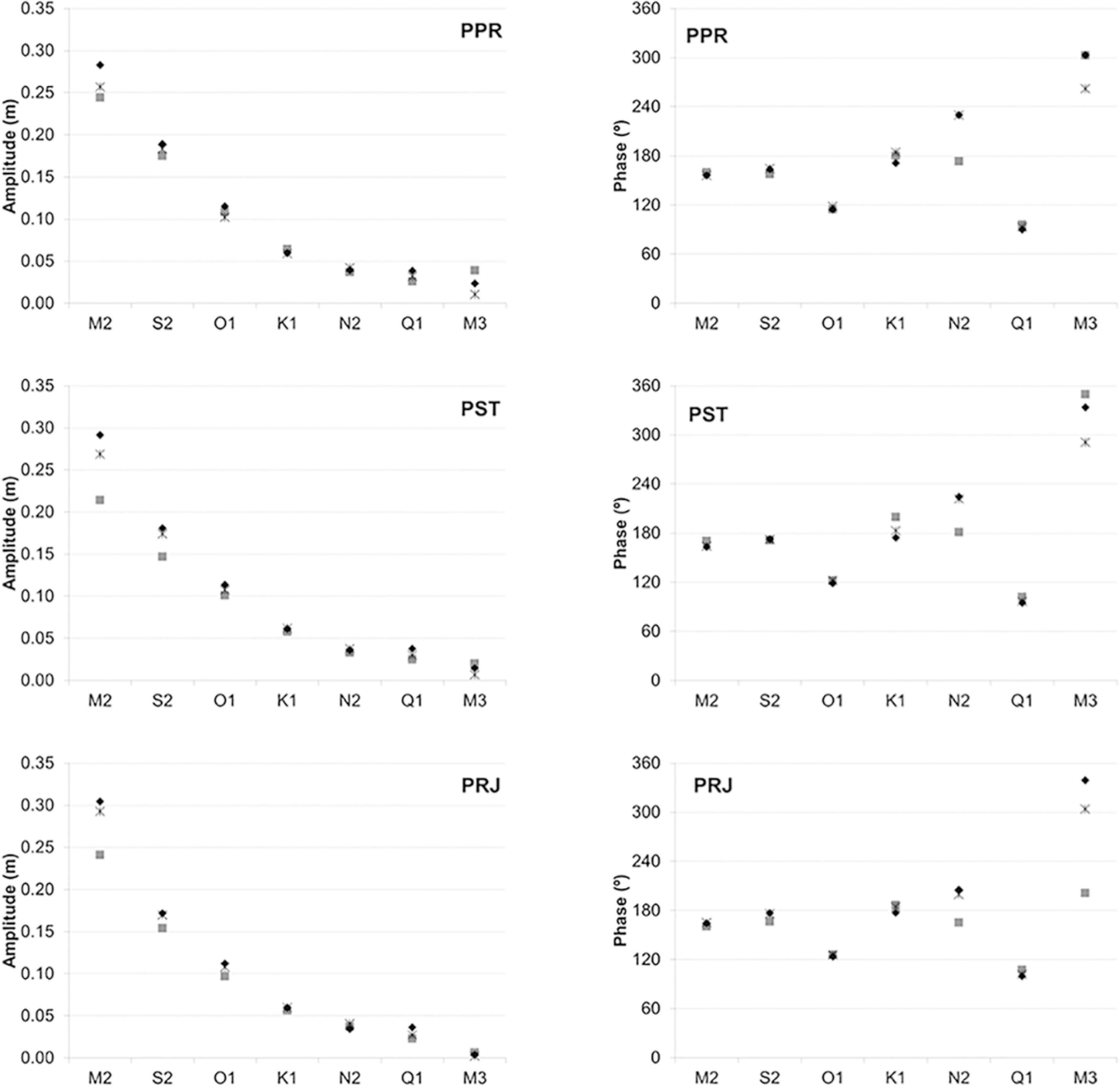
Figure 4 shows amplitudes and phases from model results and data of the three most important diurnal (O1, K1, Q1) and semidiurnal (M2, S2, N2) tidal constituents, besides M3, at three sites on the south-eastern Brazilian shelf (PPR, PST, PRJ). In addition, data from FES2012 were included as reference. The M2 constituent presented larger amplitudes (4 - 8 cm) than observed in the data, even in the FES2012 solution (1 - 5 cm), suggesting that these differences arose in part thanks to the boundary conditions. However, the M2 amplitudes obtained from the local model results (shown in next section) agreed well with the data analysis of tidal gauges inside the estuarine system, probably due to the increase in the resolution of the nested grids.

Figure 4
Amplitudes and phases of the three most important diurnal and semidiurnal tidal constituents on the south-eastern Brazilian shelf. ■ Data *Fes2012 ♦ Model.

The model's results for S2 amplitudes are slightly higher than the data's (1 - 3 cm), as well as those of FES2012. A similar pattern is observed for N2 phases, which showed the largest phase differences between the constituents analyzed (40º - 56º); with the exception of M3 in PRJ, where phase data differ greatly both from those of other stations and FES2012. M3 amplitudes from the model's results at these three sites are in general twice the values of FES2012, decreasing the relative differences of the data. M3 phases are well represented by the model, mainly at the site where M3 is more prominent (PPR). The relative differences for amplitude and absolute differences for phase between the model's results and tidal gauge data on the shelf are presented in Table 4.

Table 4
Relative differences for amplitude (%) and absolute differences for phase (°) between model results and tidal gauge data on the shelf.

Tidal Gauges	M2	S2	O1	K1	N2	Q1	M3
PPR	15.9%	7.9%	6.5%	-7.0%	6.2%	47.7%	-40.0%
	-3.7°	6.0°	-0.1°	-8.5°	56.3°	-5.7°	0.6°
PST	36.1%	22.9%	12.5%	5.0%	9.1%	49.6%	-28.0%
	-7.2°	1.6°	-3.3°	-24.9°	43.2°	-6.9°	-15.9°
PRJ	26.3%	11.6%	15.4%	6.4%	-7.0%	57.8%	-40.0%
	3.9°	10.4°	-1.9°	-9.6°	40.2°	-7.4°	137.6°

Local Model

The six most important tidal constituents observed in five tidal gauges located in the Paranaguá estuarine system (Figure 1) were investigated for the scenarios described in section 4.3. Figure 5 shows the results of amplitudes and phases compared with data. According to the amplitudes obtained from the tidal gauge data, the M3 constituent is among the fifth most important at the estuary mouth (Galheta) and is the third most important in the intermediate zone (Ilha das Cobras), with higher amplitudes than all the diurnal constituents. In the upper parts of the estuarine system, the amplitudes of overtides and compound tides become larger, due to an increase in the importance of the nonlinear terms in the momentum and continuity equations. The first overtide of M2 (M4) is the third most important constituent in Antonina and Guaraqueçaba, whereas the MS4 constituent, a compound tide of M2 and S2, becomes the sixth most important. The importance of the local tidal potential and bottom friction for tidal propagation is clearly observed by comparing the reference scenario with the scenarios that neglected these forces. The differences observed between the reference scenario and other scenarios are less significant for the diurnal constituents, showing a weaker influence of the bottom friction and local tidal potential.

Figure 5
Amplitudes and phases of the most important tidal constituents in the tidal gauges located at Paranagua estuary. ■ Data ♦ Reference (rugosity 2.5x10^-3 m) + Without friction (rugosity 1.0x10^-11 m) ◊ Without local tidal potential * Enhanced grid resolution (Level 5).

The relative differences for amplitude and absolute differences for phase between the different scenarios and tidal gauge data are presented in Table 5, taking the five most important constituents in the Paranaguá estuarine system into consideration. The results confirmed the importance of the local tidal potential in the proper simulation of the tidal propagation in local models through downscaling from a large scale domain. M2, S2 and M3 presented significantly smaller amplitudes when compared with data and the reference scenario, which means that the local tidal potential interacts positively with the open boundary tidal forcing, amplifying these constituents. The opposite was ascertained for M4, with attenuated amplitudes. As M4 is not generated from the tidal potential, the differences observed in its amplitudes and phases are derived from differences obtained in M2 when the local tidal potential is ignored. The results suggest that the M4 wave propagated from the open boundary conditions interacts negatively with the M4 generated locally when the local tidal potential of M2 is taken into account.

Table 5
Relative differences for amplitude (%) and absolute differences for phase (°) between the different scenarios and tidal gauge data inside the Paranaguá estuarine system.

Tidal Gauge	Scenario	M2	S2	M4	M3	O1
Galheta	Reference	-0.7%	9.6%	6.3%	-34.2%	11.1%
		12.2°	20.4°	103.2°	-29.3°	6.1°
	Without Local	-37.4%	-24.7%	151.8%	-76.8%	6.3%
	Tidal Potential	30.7°	31.6°	28.2°	65.2°	7.1°
	Without Friction	20.9%	34.5%	-61.3%	-2.8%	22.4%
		7.8°	15.4°	131.7°	-12.1°	-0.2°
	Enhanced Grid	7.4%	15.3%	66.2%	-12.6%	12.2%
	Resolution	-0.9°	7.7°	99.4°	-47.2°	-1.5°
Paranaguá	Reference	-3.1%	8.2%	-15.2%	-45.2%	14.1%
		17.0°	20.6°	97.7°	-6.3°	10.6°
	Without Local	-39.9%	-30.4%	113.9%	-81.1%	5.8%
	Tidal Potential	38.6°	34.8°	16.1°	84.6°	12.9°
	Without Friction	22.3%	38.8%	92.3%	9.8%	22.8%
		-4.4°	-1.7°	102.9°	-25.2°	-0.6°
	Enhanced Grid	-6.0%	2.9%	4.8%	-44.3%	9.2%
	Resolution	7.3°	12.7°	81.9°	-22.5°	6.7°
Ilha das Cobras	Reference	-8.4%	16.2%	-18.6%	-53.8%	-4.2%
		16.5°	31.5°	100.5°	-20.4°	10.8°
	Without Local	-42.8%	-23.3%	108.9%	-83.8%	-10.2%
	Tidal Potential	36.7°	43.9°	21.1°	71.2°	12.3°
	Without Friction	15.0%	48.9%	57.5%	-10.2%	3.5%
		-0.8°	13.4°	123.8°	-30.0°	1.3°
	Enhanced Grid	-8.4%	13.3%	12.3%	-49.1%	-6.8%
	Resolution	5.9°	21.9°	86.0°	-38.4°	6.0°
Antonina	Reference	-1.2%	7.6%	-7.0%	-42.6%	9.0%
		14.0°	17.0°	88.2°	-26.2°	8.8°
	Without Local	-39.2%	-32.2%	133.0%	-80.8%	-0.2%
	Tidal Potential	36.8°	34.6°	4.5°	65.5°	12.4°
	Without Friction	13.7%	27.8%	103.2%	3.6%	-4.5%
		-14.2°	-12.4°	74.3°	-59.4°	-1.5°
	Enhanced Grid	-14.2%	-5.3%	3.8%	-49.0%	-2.7%
	Resolution	10.0°	17.1°	80.7°	-31.9°	11.2°
Guaraqueçaba	Reference	-12.8%	20.4%	-36.7%	-55.8%	6.1%
		29.0°	33.6°	114.4°	2.7°	18.6°
	Without Local	-45.3%	-20.4%	68.2%	-84.7%	-1.4%
	Tidal Potential	49.6°	48.0°	30.3°	95.6°	21.5°
	Without Friction	12.2%	61.8%	11.8%	-9.4%	16.4%
		5.4°	9.0°	124.5°	-15.2°	5.9°
	Enhanced Grid	-24.0%	-2.1%	-41.8%	-61.4%	2.6%
	Resolution	-7.7°	-1.8°	20.7°	-63.2°	-0.8°

M3 amplitudes become 30% to 40% closer to data in the reference scenario than in the scenario that ignores the local tidal potential. However, a relative error of between -34% and -56% is still found. These errors are of the same order of magnitude (-40%) as that found in the tidal gauges on the shelf shown in Table 4, indicating that they arose outside the estuarine system in the regional model. A considerable improvement when considering the local tidal potential was also observed in tidal phase, especially for M3. The exception was M4, which presented better phase results for the scenario without this force.

As expected, the scenario in which the bottom friction was ignored presented higher amplitudes for the linear constituents than did the reference scenario. The nonlinear M4 constituent also presented higher amplitudes in this scenario (Galheta is the only exception). Thus, it may be stated that the nonlinear friction term in the momentum equation is not greatly important for M4 generation along the Paranaguá estuarine system. This is in agreement with other studies that attributed greater importance to the nonlinear continuity term for M4. On the other hand, the bottom friction is important for the MS4 constituent, increasing its amplitudes by two times in Guaraqueçaba and four times in Antonina.

M3 amplitudes show a better fit with data in the scenario ignoring bottom friction than in the reference scenario, with differences of the order of 1 cm. However, the other most important constituents, namely M2, S2 and M4, presented much larger differences in amplitudes. This means that M3 amplitudes in the model cannot be fitted to data by only adjusting the bottom roughness length, as the other constituents would be overestimated. Thus, the error might arise from other sources, such as the open boundary conditions of FES2012.

The improvement in grid resolution from 600 m to 120 m (Level 5) presented the largest differences from the reference scenario in the upper zones (Antonina and Guaraqueçaba), where the amplitudes of the main constituents (M2 and S2) decreased significantly. This outcome may be explained by the inclusion of the intertidal zones in Level 5, which enlarged the area for tidal propagation. The amplitudes can be adjusted in the future by considering a drag coefficient for water flow in mangrove zones. However, an improvement was obtained in the M2 and S2 phases in the Laranjeiras bay (Guaraqueçaba). This effect may be a consequence of a better characterization of estuarine channels. The mean absolute error of amplitudes and phases for the different scenarios is presented in Table 6.

Table 6
Mean absolute error of amplitudes (cm) and phases (°) for the five most important tidal constituents.

	Scenario	M2	S2	M4	M3	O1
Mean Absolute Error	Reference	2.6	3.6	2.8	6.9	1.0
		17.7°	24.6°	100.8°	17.0°	11.0°
	Without Local	19.4	7.9	17.1	11.8	0.6
	Tidal Potential	38.5°	38.6°	20.0°	76.4°	13.2°
	Without Friction	7.8	12.4	10.2	1.1	1.6
		6.5°	10.4°	111.4°	28.4°	1.9°
	Enhanced Grid	5.9	2.2	3.3	6.8	0.8
	Resolution	6.4°	12.2°	73.7°	40.6°	5.2°

Baroclinic Model

The validation of salinity and temperature in the regional model domain (Level 2), with Argo float profiles, is shown in Figures 6 and 7 for a summer and winter period, respectively. For instance, comparisons between profiles measured by individual floats and simulated by the model at the same location are shown, besides the T-S diagram that identifies the different water masses. The density stratification was adequately simulated by the model. Statistics for a 30-day period in summer and winter considering all the Argo floats are also shown, with Pearson's correlation coefficient very close to 1 and, in general, a small Bias and RMSE for both temperature and salinity.

Figure 6
Salinity and temperature results compared with Argo floats profiles in summer (above). Statistics between results and Argo floats profiles in January 2013 (below).

Figure 7
Salinity and temperature results compared with Argo floats profiles in winter (above). Statistics between results and Argo floats profiles in July 2013 (below).

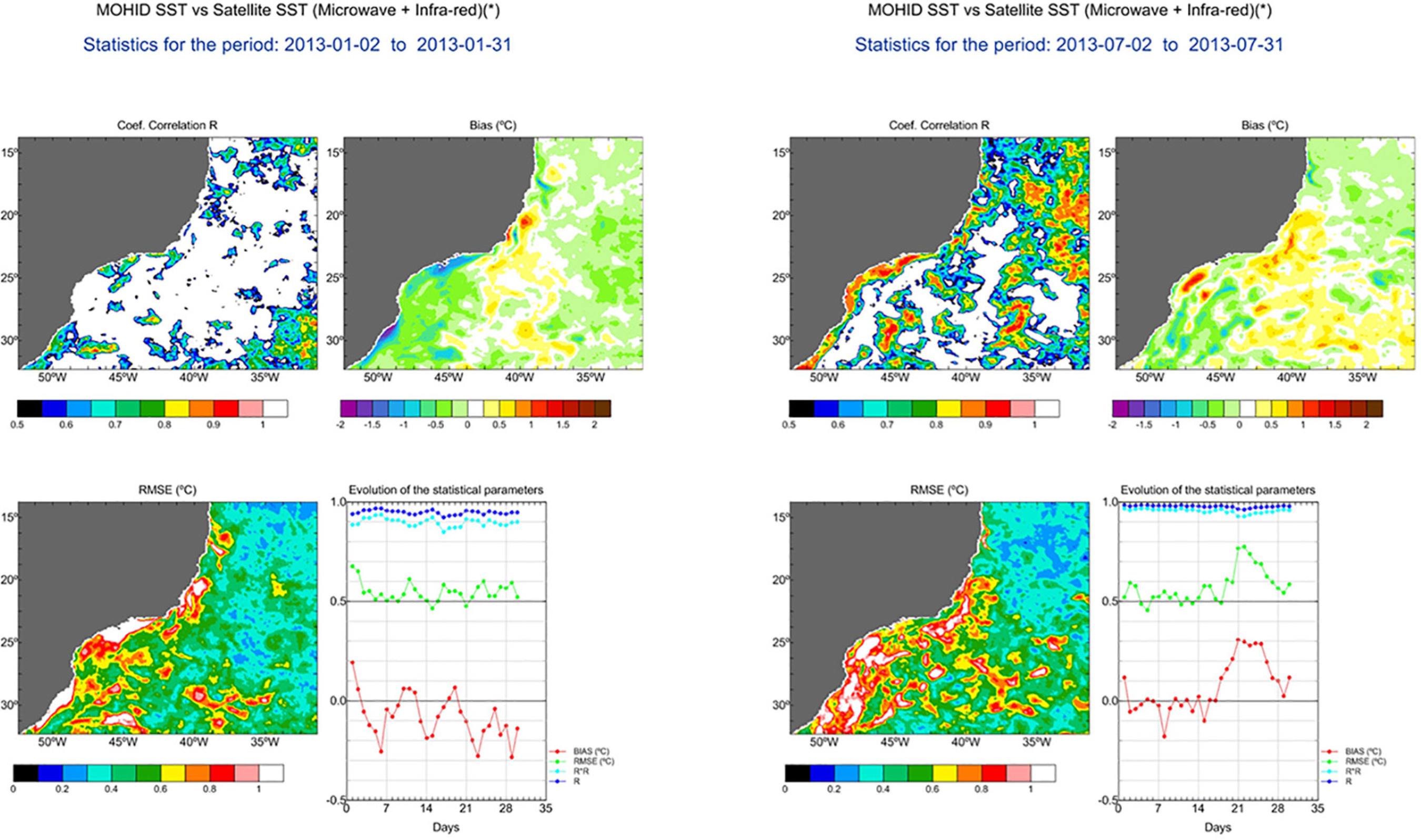
SST results are compared with satellite measurements in Figure 8. It is possible to observe the southward heat transport due to the Brazil current, which is also responsible for upwelling along the shelf break. The strong flows from Rio de la Plata also influence the temperatures observed near the coast in the southern part of the domain. Figure 9 shows the validation performed for 30 days in summer (January) and winter (July), with generally strong correlation and small Bias and RMS. The major differences in relation to measurements were found near the coast, possibly due to the lack of interaction between the shelf sea and estuarine systems in the regional model.

Figure 8
SST (ºC) results compared with satellite measurements in summer (left) and in winter (right).

Figure 9
Statistics between SST (ºC) results and satellite measurements in January 2013 (left) and July 2013 (right).

DISCUSSION

We demonstrated that the methodology of downscaling with nested models is applicable to the south-eastern Brazilian shelf and the Paranaguá estuarine system, representing an important progress as compared to previous studies (e.g. CAMARGO; HARARI, 2003). The results confirmed the importance of the local tidal potential to properly simulate the tidal propagation in local models, following a downscaling from a large scale domain. The validation of temperature and salinity with Argo float profiles, as well as SST with satellite measurements, indicated that the regional model can represent the patterns observed on the south-eastern Brazilian shelf, such as the upwelling process caused by the Brazil current. Thus, the regional model is capable of providing adequate boundary conditions for the local model.

The inclusion of the M3 term in the local tidal potential contributed significantly to a better representation of its amplitudes and phases in the model domain. This outcome agrees with the conclusions of other modelling studies in areas where tidal resonance is observed (e.g. WIJERATNE et al., 2012). Taking 100 m as an average depth for the shelf, the wavelength for M3 is approximately 933 km. When the shelf width is about one quarter of the wavelength (233 km for M3), resonance phenomena may occur. This condition is satisfied in the broader parts of the south-eastern Brazilian shelf. The M3 resonance is also seen in the Great Australian Bight.

The differences between the harmonic constituents found in model results and data arose in part because of the open boundary tidal forcing. The constant development of a more accurate global tidal atlas will contribute to a further improvement in the model results of tidal propagation. Future studies are needed to validate water temperature and salinity in the Paranaguá estuarine system, which depends on a representative set of local data's becoming available. Furthermore, the results of the local model can be used to provide boundary conditions for the regional model in a two-way nesting, allowing an improvement in the results of water temperature and salinity measurement near the coast. The simulation of storm surges also needs to be addressed in future studies, in view of the importance of these events for the water level oscillations observed in this estuarine system, found to be of the same order of magnitude as the tide amplitude.

The methodology described in this study can be replicated for other important estuarine systems, such as Guanabara Bay and Santos Bay, located on the south-eastern Brazilian shelf, by using the results of the same regional model as open boundary conditions. The numerical model developed for the Paranaguá estuarine system with a high grid resolution (120 m) can be used for the investigation of important questions, such as the transport of sediments and water quality. Furthermore, the model was developed with a view to future nowcast/forecast simulations, useful for several activities, such as navigation and response to emergencies (e.g., oil spills). Two harbors are located in the Paranaguá estuarine system (those of Paranaguá and Antonina); the harbor of Paranaguá is one of the most important Brazilian harbors in terms of financial turnover.

Finally, we have confirmed that the application of a numerical modelling system adopting a downscaling approach is capable of simulating processes of different spatial scales on the south-eastern Brazilian shelf, providing accurate boundary conditions to the Paranaguá estuarine system. This thus represents a valuable tool and significant progress for modelling studies in this area.

ACKNOWLEDGEMENTS

The authors are grateful to the Brazilian Navy for providing the tidal gauge data, to ENVEX Engenharia e Consultoria Ambiental for providing the bathymetry data of the Paranaguá estuarine system and to all the MARETEC team for their technical support. We would also thank Isabella Ascione Kenov for providing the MATLAB scripts for processing FES2012 data. The first author is financed by CNPQ (Brazil) under the Ciências Sem Fronteiras program (research grant no. 237448/2012-2).

REFERENCES

• ASCIONE, K. I.; CAMPUZANO, F.; FRANZ, G.; FERNANDES, R.; VIEGAS, C.; SOBRINHO, J.; DE PABLO, H.; AMARAL, A.; PINTO, L.; MATEUS, M.; NEVES, R. Advances in modeling of water quality in estuaries. In: FINKL, C. W.; MAKOWSKI, C. (Eds.). Advances in Coastal abd Marine Resources: Remote Sensing and Modeling. Advances in Coastal and Marine Resources. Part II. Cham: Springer International Publishing, 2014. p. 237-276.
• BRICHENO, L. M.; WOLF, J. M.; BROWN, J. M. Impacts of high resolution model downscaling in coastal regions. Cont. Shelf Res., v. 87, p. 1-16, 2014.
• BUCHARD, H.; BOLDING, K.; VILLARREAL, M. R. GOTM, a General Ocean Turbulence Model. Theory, implementation and test cases. Ispra: Space Applications Institute, 1999. p. 1-103.
• CAMARGO, R.; HARARI, J. Modelagem numérica de ressacas na plataforma sudeste do Brasil a partir de cartas sinóticas de pressão atmosférica na superfície. Bol. Inst. Oceanogr., S. Paulo, v. 42, n. 1-2, p. 19-34, 1994.
• CAMARGO, R.; HARARI, J. Modeling of Paranaguá estuarine complex, Brazil: tidal circulation and cotidal charts. Rev. Bras. Oceanogr., v. 51, p. 23-31, 2003.
• CAMPOS, E. J. D.; GONÇALVES, J. E.; IKEDA, Y. Water mass characteristics and geostrophic circulation in the South Brazil Bight: Summer of 1991. J. Geophys. Res., v. 100, n. 9, p. 18537-18550, 1995.
• CAMPOS, E. J. D.; VELHOTE, D.; DA SILVEIRA, I. C. A. Shelf break upwelling driven by Brazil Current cyclonic meanders. Geophys. Res. Let., v. 27, p. 751-754, 2000.
• CANAS, A.; SANTOS, A.; LEITÃO, P. Effect of large scale atmospheric pressure changes on water level in the Tagus Estuary. J. Coast. Res., v. 56, p. 1627-1631, 2009.
• CARRÈRE, L.; LYARD, F.; CANCET, M.; GUILLOT, A.; ROBLOU, L. FES2012: a new global tidal model taking advantage of nearly 20 years of altimetry. In: Paper presented at the Symposium 20 Years of Progress in Radar Altimetry. Venice: Esa Publication, 2012.
• CUMMINS, P. F.; KARSTEN, R. H.; ARBIC, B. K. The semi-diurnal tide in Hudson Strait as a resonant channel oscillation. Atmos. Ocean, v. 48, n. 3, p. 163-176, 2010.
• ENGEDAHL, H. Use of the flow relaxation scheme in a three-dimensional baroclinic ocean model with realistic topography. Tellus, v. 47, n. 3, p. 365-382, 1995.
• FLATHER, R. A. A tidal model of the north-west European continental shelf. Mém. Soc. R. Sci. Liège, v. 10, p. 141-164, 1976.
• FRANZ, G.; PINTO, L.; ASCIONE, I.; MATEUS, M.; FERNANDES, R.; LEITÃO, P.; NEVES, R. Modelling of cohesive sediment dynamics in tidal estuary systems: case study of Tagus estuary, Portugal. Estuar. Coast. Shelf Sci., v. 151, p. 34-44, 2014a.
• FRANZ, G.; FERNANDES, R.; DE PABLO, H.; VIEGAS, C.; PINTO, L.; CAMPUZANO, F. J.; ASCIONE, I.; LEITÃO, P.; NEVES, R. Tagus Estuary hydro-biogeochemical model: Inter-annual validation and operational model update. 3.as Jornadas de Engenharia Hidrográfica. Lisbon: Extended abstracts, 2014b. p. 103-106.
• FOREMAN, M. G. G. Manual for Tidal Heights Analysis and Prediction. Pacific Marine Science Report, 77-10. Sydney: Institute of Ocean Sciences, 1996.
• GARRETT, C. Tidal resonance in the Bay of Fundy and Gulf of Maine. Nature, v. 238, n. 5365, p. 441-443, 1972.
• GOUILLON, F.; MOREY, S. L.; DUKHOVSKOY, D. S.; O'BRIEN, J. J. Forced tidal response in the Gulf of Mexico. J. Geophys. Res., v. 115, n. c10, 2010.
• HARARI, J.; CAMARGO, R. Simulação da propagação das nove principais componentes de maré na plataforma sudeste brasileira através de modelo numérico hidrodinâmico. Bol. Inst. Oceanogr. S. Paulo, v. 42, n. 1, p. 35-54, 1994.
• HUTHNANCE, J. M. On shelf-sea 'resonance' with application to Brazilian M3 tides. Deep-Sea Res., v. 27, n. 5, p. 347-366, 1980.
• KANTHA, L.; WHITMER, K.; BORN, G. The inverted barometer effect in altimetry: a study in the North Pacific. TOPEX/Poseidon Res. News, v. 2, p.18-23, 1994.
• KANTHA, L. H.; CLAYSON, C. A. Numerical Models of Oceans and Oceanic Processes. International Geophysics Series. New York: Academic Press, 2000.
• LEFÈVRE, F.; LYARD, F. H.; LE PROVOST, C.; SCHRAMA, E. J. O. FES99: A Global Tide Finite Element Solution Assimilating Tide Gauge and Altimetric Information. J. Atmos. Oceanic Technol., v. 19, p. 1345-1356, 2002.
• LEITÃO, P. C.; MATEUS, M.; BRAUNSCHWEIG, F.; FERNANDES L.; NEVES, R. Modelling coastal systems: the MOHID Water numerical lab. In: NEVES, R.; BARETTA, J.; MATEUS, M. (eds.). Perspectives on Integrated Coastal Zone Management in South America. Lisbon: IST Press. p. 77-88, 2008.
• LYARD, F.; LEFÈVRE, F.; LETELLIER, T.; FRANCIS, O. Modelling the global ocean tides: modern insights from FES2004. Ocean Dyn., v. 56, n. 5, p. 394-415, 2006.
• MARTINS, F.; LEITÃO, P. C.; SILVA, A.; NEVES, R. 3D modelling in the Sado estuary using a new generic vertical discretization approach. Oceanol. Acta, v. 24, p. 51-62, 2001.
• MARTINSEN, E. A.; ENGEDAHL, H. Implementation and testing of a lateral boundary scheme as an open boundary condition in a barotropic ocean model. Coast. Eng., v. 11, n. 5-6, p. 603-627, 1987.
• MATEUS, M.; RIFLET, G.; CHAMBEL, P.; FERNANDES, L.; FERNANDES, R.; JULIANO, M.; CAMPUZANO, F.; PABLO, H.; NEVES, R. An operational model for the West Iberian coast: products and services. Ocean Sci., v. 8, n. 4, p. 713-732, 2012.
• MARALDI, C.; CHANUT, J.; LEVIER, B.; AYOUB, N.; DE MEY, P.; REFFRAY, G.; LYARD, F.; CAILLEAU, S.; DRÉVILLON, M.; FANJUL, E. A.; SOTILLO, M. G.; MARSALEIX, P. NEMO on the shelf: assessment of the Iberia-Biscay-Ireland configuration. Ocean Sci., v. 9, p. 745-771, 2013.
• MESQUITA, A. R.; HARARI, J. On the harmonic constants of tides and tidal currents of the South-eastern Brazilian shelf. Cont. Shelf. Res., v. 23, n. 11-13, p. 1227-1237, 2003.
• NOERNBERG, M. A.; LAUTERT, L. F. C.; ARAÚJO, A. D.; MARONE, E.; ANGELOTTI, R.; NETTO JR., J. P. B.; KRUG, L. A. Remote sensing and GIS integration for modelling the Paranaguá Estuarine Complex - Brazil. J. Coastal Res., v. SI39, p. 1627-1631, 2006.
• ODAMAKI, M. Co-oscillating and independent tides of the Japan Sea. J. Oceanogr. Soc. Japan, v. 45, n. 3, p. 217-232, 1989.
• PAIRAUD, I. L.; LYARD, F.; AUCLAIR, F.; LETELLIER, T.; MARSALEIX, P. Dynamics of the semi-diurnal and quarter-diurnal internal tides in the Bay of Biscay. Part 1: barotropic tides. Cont. Shelf Res., v. 28, n. 10-11, p. 1294-1315, 2008.
• PARKER, B. B. The relative importance of the various nonlinear mechanisms in a wide range of tidal interactions (Review). In: PARKER, B. B. (Ed). Tidal Hydrodynamics. New York: John Wiley & Sons, 1991. p. 237-268.
• PAWLOWICZ, R.; BEARDSLEY, B.; LENTZ, S. Classical tidal harmonic analysis including error estimates in Matlab using T_Tide. Comput. Geosci., v. 28, p. 929-937, 2002.
• PEREIRA, A. F.; CASTRO, B. M. Internal tides in the southwestern Atlantic off Brazil: observations and numerical modelling. J. Phys. Oceanogr., v. 37, n. 6, p. 1512-152, 2007a.
• PEREIRA, A. F.; CASTRO, B. M.; CALADO, L.; SILVEIRA, I. C. A. Numerical simulation of M2 internal tides in South Brazil Bight and their interaction with the Brazil Current. J. Geophys. Res., v. 112, n. C04009, 2007b.
• PUGH, D. T.; WOODWORTH, P. L. Sea-level science: understanding tides, surges tsunamis and mean sea-level changes. Cambridge: Cambridge University Press, 2014. 407 p.
• VILLARREAL, M. R.; BOLDING, K.; BURCHARD, H.; DEMIROV, E. Coupling of the GOTM turbulence module to some three-dimensional ocean models. In: BAUMERT, H. Z.; SIMPSON, J. H.; SÜNDERMANN, J. (Eds.). Marine Turbulence: Theories, Observations and Models. Cambridge: Cambridge University Press , 2005. p. 225-237
• WIJERATNE, E. M. S.; PATTIARATCHI, C. B.; ELIOT, M.; HAIGH, I. D. Tidal characteristics in Bass Strait, south-east Australia. Estuar. Coast. Shelf Sci., v. 114, p. 156-165, 2012.

Publication Dates

• Publication in this collection
  Jul-Sep 2016