Simulation of deterministic compartmental models for infectious diseases dynamics

Abstract

Infectious diseases are caused by pathogenic microorganisms and can spread through different ways. Mathematical models and computational simulation have been used extensively to investigate the transmission and spread of infectious diseases. In other words, mathematical model simulation can be used to analyse the dynamics of infectious diseases, aiming to understand the effects and how to control the spread. In general, these models are based on compartments, where each compartment contains individuals with the same characteristics, such as susceptible, exposed, infected, and recovered. In this paper, we cast further light on some classical epidemic models, reporting possible outcomes from numerical simulation. Furthermore, we provide routines in a repository for simulations.

Keywords
Compartmental model; computational simulation; infectious diseases; COVID-19

1. Introduction

Infectious diseases have caused epidemics with devastating effects, for instance influenza A virus sub-type H1N1 [¹] and smallpox [²]. Infectious disease with pandemic potential is one of the greatest challenges of the health system. Recently, the World Health Organization declared COVID-19 [³, ⁴] as a pandemic. The mortality depends on many factors such as number of infected people, virulence, and prevention efforts [⁵]. Various infectious diseases can come in waves, e.g., the first three waves of avian influenza A (H7N9) virus circulation [⁶]. Kissler et al. [⁷] projected that recurrent outbreaks of COVID-19 will probably happen.

Epidemiological models [⁸] have been proposed to analyse the spread of infectious diseases in host populations [⁹]. In 1760, Bernoulli [¹⁰] proposed a model to describe the impact of variolation. In 1906, a mathematical model to explain the epidemic of measles was introduced by Hamer [¹¹].

The SI model [¹²] describes the evolution of susceptible S and infected I individuals, respectively. A model was proposed by Ross [¹³] in 1916 for malaria. In the Ross model, known as SIS model [¹⁴], susceptible become infected and infected recover without immunity. Kermack and McKendrick [¹⁵] introduced a model, known as SIR model, in which the removed can be recovered, immune, or dead. The SIRS model [¹⁶] was obtained when a waning immunity was incorporated. In the SEIR model [¹⁷] there are four states, where E corresponds to exposed, namely a latency period is considered. It has been applied to measles [¹⁸] and rubella [¹⁹]. The SEIRS model [²⁰] considers individuals that are transferred from the recovered to the susceptible compartments.

One of the different types of controls of epidemic is the vaccination. The vaccination controls have as main objective to remove by immunity the population from the susceptible state [²¹]. Gao et al. [²²] demonstrated that pulse vaccination can be an effective strategy for the elimination of infectious diseases. Investigating the transmission of tuberculosis by means of epidemiological models, Liu et al. [²³] reported that mixed vaccination gives a rapid control.

When there is no vaccine for the infectious disease, the control strategies are based on quarantine and isolation, for instance the COVID-19 epidemics [²⁴]. Law et al. [²⁵] studied a time-varying SIR model for the transmission dynamics of COVID-19. Prem et al. [²⁶] reported that the magnitude of the epidemic peak can be reduced through sustained physical distancing. Feng [²⁷] analysed the final and peak epidemic sizes considering quarantine and isolation in SEIR models. Recently, Boldog et al. [²⁸] analysed the risk assessment of novel coronavirus outbreaks outside China by means of an extension of a standard SEIR model.

Stochastic mathematical models have been considered in prediction of the spread of several infectious diseases [²⁹]. The law of mass-action has been used for almost a century in epidemiology to describe the contact rate of individuals. This law originated in practice and theory of chemical reaction kinetics [³⁰]. Tomé and Oliveira [¹⁴] presented models for epidemic spreading and showed the analogy between the spreading of a disease with a critical phase transition. They also analysed the epidemic curve, which is a graphical representation of the number of identified cases over a period of time.

In this work, we focus on the simulation of different deterministic models that have been used to describe infectious disease dynamics. We provide routines in a repository [³¹] to assist students with their first steps about computer simulations of mathematical models in epidemiology. The reader can find mathematical details in Ref. [¹⁴]. We show the dynamical behaviours predict by some mathematical models, such as SI, SIS, SIR, SIRS, SEIR, and SEIRS. We present an application of the SIR model in COVID-19 for the parameters obtained from China according to Ref. [³²]. Considering the SEIR model, we show the impact of easing restriction on the infection rate that was reported in Ref. [³³].

2. The SI Model

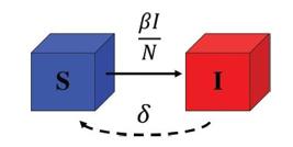
The SI model describes the dynamical behaviour of transmitted diseases [³⁴] with interactions among infected and susceptible people. In this model, vital processes are not considered, such as rates of birth and mortality. Figure 1 displays the diagram of the SI model, where the population is divided into susceptible and infected individuals. After infected, the individual does not return to the susceptible class, for instance herpes that is spread from person to person by the virus Herpesviridae.

Figure 1
Compartment diagram of the SI model, where S and I are the numbers of susceptible and infected individuals, respectively, and β (in units of 1/day) is the effective contact rate of the disease.

The SI model is given by

(1) $${\displaystyle \frac{dS}{dt}}=-{\displaystyle \frac{\beta SI}{N}},$$

(2) $${\displaystyle \frac{dI}{dt}}={\displaystyle \frac{\beta SI}{N}},$$

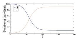
where N = S + I is the total population and β is the effective contact rate of the disease. Figure 2 exhibits the time evolution (in days) of S (blue line) and I (red line) for β = 0.1. With time, every susceptible individual becomes infected.

Figure 2
Time evolution of S (blue line) and I (red line) for N = 1000, S(0) = 995, I(0) = 5, and β = 0.1.

3. The SIS Model

In the SIS model [³⁵, ³⁶], which was studied recently [¹⁴, ²⁹], the infected individuals can become susceptible, however, there is no long-lasting immunity. Due to this fact, an individual can have recurrent infections, such as common cold (rhinoviruses) and influenza, as well as sexually transmitted diseases, for instance chlamydia and gonorrhoea. In Fig. 3, we see a schematic representation of the compartment diagram related to the SIS model.

Figure 3
Compartment diagram of the SIS model, where S and I are the numbers of susceptible and infected individuals, respectively, β (in units of 1/day) is the infectious rate, and δ (in units of 1/day) is the rate in which the infected individuals recover to the susceptible state.

The SIS model is written as

(3) $${\displaystyle \frac{dS}{dt}}=-{\displaystyle \frac{\beta SI}{N}}+\delta I,$$

(4) $${\displaystyle \frac{dI}{dt}}={\displaystyle \frac{\beta SI}{N}}-\delta I,$$

where the infected individual goes to the susceptible state with a rate δ. In Fig. 4, we consider β = 0.1 and δ = 0.01 for N=1000. The SIS model has two stable equilibria, one for I = 0 and another for I = N(1−δ/β).

Figure 4
Time evolution of S (blue line) and I (red line) for N=1000, S(0) = 995, I(0) = 5, β = 0.1, and δ = 0.01.

4. The SIR Model

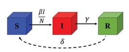
In 1927, Kermack and McKendrick [¹⁵] proposed the SIR model, a mathematical model of spread of an infectious disease within a population, studied recently [¹⁴, ²⁹]. They considered three compartments, in which the susceptible individuals go to the infectious compartment according to an infectious rate and, depending on the recover rate, the infected individual recover and develop immunity, as shown in Fig. 5.

Figure 5
Compartment diagram of the SIR model, where S, I, and R are the numbers of susceptible, infected, and recovered individuals, respectively, β (in units of 1/day) is the infectious rate, and γ (in units of 1/day) is the rate in which the infected individuals recover.

The SIR model was introduced to explain the rapid increase of infected individuals, as verified in epidemics such as the cholera and the plague. The mathematical model is given by

(5) $${\displaystyle \frac{dS}{dt}}=-{\displaystyle \frac{\beta SI}{N}},$$

(6) $${\displaystyle \frac{dI}{dt}}={\displaystyle \frac{\beta SI}{N}}-\gamma I,$$

(7) $${\displaystyle \frac{dR}{dt}}=\gamma I,$$

where γ is the recovery rate and N = S + I + R. The behaviour of the infectious class has a dependence on the parameter R₀ = β/γ, known as reproduction ratio. R₀ is an important threshold quantity that describes the transmissibility or contagiousness of pathogenic microorganisms [³⁷]. In a susceptible group of individuals, it gives the expected number of secondary cases of infections due to an infected individual. The pathogenic microorganism is able to invade the population of susceptible individuals if R₀ > 1. The births and deaths are not considered due to the fact that the infection and recovery rates are fast.

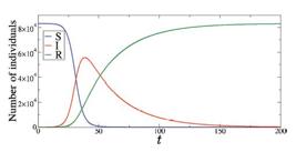
Figure 6 shows the time evolution (in days) of S (blue line), I (red line), and R (green line) for N=1000, β = 0.2, and γ = 0.05. As initial conditions, we consider S(0) = 995 and I(0) = 5. We see that the infected population reaches a peak while the susceptible individuals decrease and recovered ones increase. After the peak, the number of infected individuals decreases.

Figure 6
Time evolution of S (blue line), I (red line), and R (green line) for N=1000, S(0) = 995, I(0) = 5, β = 0.2, and γ = 0.05.

In 2020, the SIR model was utilised by Cooper et al. [³²] to study the spread of COVID-19 in different communities. They analysed data recorded between January and June 2020 from China, South Korea, India, Australia, Italy, and the state of Texas in the USA. It was demonstrated that the SIR model can provide a theoretical framework to study how the COVID-19 virus spreads within communities. Figure 7 displays the time evolution of S (blue line), I (red line), and R (green line) for N=83132, S(0) = 83127, I(0) = 5, β = 0.35, and γ = 0.035, where the parameters are selected according to Ref. [³²] for China.

Figure 7
Time evolution of S (blue line), I (red line), and R (green line) for N=83132, S(0) = 83127, I(0) = 5, β = 0.35, and γ = 0.035.

5. The SIRS Model

The SIRS model has been studied by various authors [³⁸, ³⁹] and studied recently [¹⁴, ¹⁶, ²⁹]. Figure 8 exhibits the process diagram for the SIRS model. In this model, the recovery can generate temporary immunity, and as a consequence the recovered individuals return to the susceptible class after some time. The loss of immunity is observed in smallpox, tetanus, and influenza.

Figure 8
Compartment diagram of the SIRS model, where S, I, and R are the numbers of susceptible, infected, and recovered individuals, respectively, β (in units of 1/day) is the infectious rate, γ (in units of 1/day) is the rate in which the infected individuals recover, δ (in units of 1/day) is the rate in which the recovered individuals return to the susceptible class.

The SIRS model is given by

(8) $${\displaystyle \frac{dS}{dt}}=-{\displaystyle \frac{\beta SI}{N}}+\delta R,$$

(9) $${\displaystyle \frac{dI}{dt}}={\displaystyle \frac{\beta SI}{N}}-\gamma I,$$

(10) $${\displaystyle \frac{dR}{dt}}=\gamma I-\delta R,$$

where δ is the rate in which the recovered individuals return to the susceptible class after losing the immunity and N = S + I + R.

In Fig. 9, the blue, red, and green lines correspond to the time evolution (in days) of S, I, and R, respectively. We see the persistence of the infected population due to the transfer of individuals from the recovery class to the susceptible one.

Figure 9
Time evolution of S (blue line), I (red line), and R (green line) for N=1000, S(0) = 995, I(0) = 5, β = 0.4, γ = 0.2, and δ = 0.005. The inset figure corresponds to the magnification of the infected individuals.

6. The SEIR Model

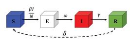
One of the compartmental models of infectious diseases is the SEIR model, studied recently [¹⁴, ²⁹]. In this model, the individuals are separated into four compartments. The SEIR model assumes people in the susceptible (S), exposed (E), infected (I), and recovered (R) states, as shown in Fig. 10.

Figure 10
Compartment diagram of the SEIR model, where S, E, I, and R are the numbers of susceptible, exposed, infected, and removed individuals, respectively, β (in units of 1/day) is the infectious rate, ω (in units of 1/day) is the coefficient of migration rate, and γ (in units of 1/day) is the rate in which the infected individuals recover.

The people move from S to E due to direct or indirect contact. In the E stage, the people are infected but are not infectious, namely an latent period. The infected individuals are recovered. The SEIR model was used by Carcione et al. [⁴⁰] to simulate the COVID-19 epidemic.

The SEIR model is written as

(11) $${\displaystyle \frac{dS}{dt}}=-{\displaystyle \frac{\beta SI}{N}},$$

(12) $${\displaystyle \frac{dE}{dt}}={\displaystyle \frac{\beta SI}{N}}-\omega E,$$

(13) $${\displaystyle \frac{dI}{dt}}=\omega E-\gamma I,$$

(14) $${\displaystyle \frac{dR}{dt}}=\gamma I,$$

where β is the coefficient of infection rate, ω is the coefficient of migration rate of latency, γ is the coefficient of migration rate, and N = S + E + I + R is the total population.

Figure 11 displays the temporal evolution (in days) of S (blue line), E (black line), I (red line), and R (green line) for β = 0.5, γ = 0.01, ω = 0.1. Initially, S decreases and E, I, and R increase. S is depleted by the epidemic and goes to zero. Both E and I exhibit peaks and R saturates when they go to zero.

Figure 11
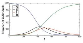
Time evolution of S (blue line), E (black line), I (red line), and R (green line) for N=1000, S(0) = 995, I(0) = 5, β = 0.5, ω = 0.1, and γ = 0.1.

Recently, Souza et al. [³³] considered the SEIR model to analyse the impact of easing restriction on the infection rate during COVID-19 pandemic. They included a parameter related to the restriction r in the SEIR model, β→β(1−r). By increasing r, the peak of infectious is delayed and the curve peak is flattened, as shown in Fig. 12(a). Figure 12(b) shows that changes in the value of r can generate a second wave, namely the increase of the number of infected individuals after few cases.

Figure 12
(a) Time evolution of I for ω = 0.2, γ = 0.25, r = 0 (red line), r = 0.2 (red dashed line), and r = 0.4 (red dotted line). (b) Time evolution of I for r = 0 (t < 14), r = 0.6 (14≤t < 365), and r = 0.2 (t ≥ 365).

7. The SEIRS Model

In the SEIRS model, the susceptible individuals first go through the exposed class before infected one. After the infectious, they are transferred to the recovered compartment and become susceptible again, as shown in Fig. 13. Denphedtnong et al. [⁴¹] used the SEIRS epidemic model to describe the spread of diseases by transports. They investigated the data of SARS (severe acute respiratory syndrome) outbreak in 2003.

Figure 13
Compartment diagram of the SEIRS model, where S, E, I, and R are the numbers of susceptible, exposed, infected, and removed individuals, respectively, β (in units of 1/day) is the infectious rate, ω (in units of 1/day) is the coefficient of migration rate, γ (in units of 1/day) is the rate in which the infected individuals recover, and δ (in units of 1/day) is the rate in which the recovered individuals return to the susceptible class.

The SEIRS model is given by

(15) $${\displaystyle \frac{dS}{dt}}=-{\displaystyle \frac{\beta SI}{N}}+\delta R,$$

(16) $${\displaystyle \frac{dE}{dt}}={\displaystyle \frac{\beta SI}{N}}-\omega E,$$

(17) $${\displaystyle \frac{dI}{dt}}=\omega E-\gamma I,$$

(18) $${\displaystyle \frac{dR}{dt}}=\gamma I-\delta R,$$

where δ is the rate in which the recovered individuals return to the susceptible class after losing the immunity.

In Fig. 14, we calculate S (blue line), E (black line), I (red line), and R (green line) for N=1000, S(0) = 995, I(0) = 5, β = 0.5, ω = 0.1, γ = 0.1, and δ = 0.03. We see that the susceptible, exposed, and infected individuals do not go to the value equal to zero over time. This occurs due to the fact that recovered individuals become susceptible again.

Figure 14
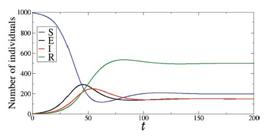
Time evolution of S (blue line), E (black line), I (red line), and R (green line) for N=1000, S(0) = 995, I(0) = 5, β = 0.5, ω = 0.1, γ = 0.1, and δ = 0.03.

8. Conclusions

Investigations about infectious diseases play a crucial role in reducing negative consequences and improving the recovery of individuals. Scientists have been carried out research in epidemiology to understand how the people are affected by transmissible diseases over time. Many different mathematical models were proposed to find epidemiological parameters and manners to prevent illness.

In this work, we present some mathematical models that have been used to describe the dynamical behaviour of infectious diseases. The models are based on individuals that are separated into compartments, such as susceptible (S), exposed (E), infected (I), and recovered (R). They focus on the prediction of the population growth or reduction in each compartment. The models depend on the parameters related to the rate in which individuals are transferred between the classes.

The SI model considers that the individuals go from the susceptible to infected states, while the SIS model assumes that there is no immunity and the infected individuals return to the susceptible compartment. In the SIR and SIRS model, it is included the class of the recovered individuals. The SEIR and SEIRS models have not only the susceptible, infected, and recovered individuals, but also the exposed ones. Recently, the SIR and SEIR models have been used in studies about the COVID-19 epidemic. The SIR, SIRS, SEIR, and SEIRS models exhibit a peak of infected people that was observed in different infection spread.

It has been demonstrated that through the intensity of restrictions associated with the control policies to reduce the infection spread, it is possible to flat the curve associated with the temporal evolution of the infected people [³³]. However, the results depend on the duration and specific time in which the restriction is applied. The peak of infections can be reduced by means of restrictions or another peak can appear after suspending the restrictions.

We provide routines in a repository for the SI, SIS, SIR, SIRS, SEIR, and SEIRS models [³¹].

Acknowledgements

This work was possible by partial financial support from the following Brazilian government agencies: CAPES, CNPq (407543/2018−0, 302903/2018−6, 420699/2018−0, 407299/2018−1, 428388/2018−3, 311168/2020−5), Fundação Araucária, and São Paulo Research Foundation (FAPESP 2018/03211−6). We would like to thank www.105groupscience.com.

References

• ^1.
  P. Spreeuwenberg, M. Kroneman and J. Paget, Am. J. Epidemiol. 187, 2561(2018).
• ^2.
  D.A. Henderson, Vaccine 29, D7 (2011).
• ^3.
  N. Chen, M. Zhou, X. Dong, J. Qu, F. Gong, Y. Han, Y. Qiu, J. Wang, Y. Liu, Y. Weiet al. , Lancet 395, 507 (2020).
• ^4.
  X. Han, Y. Cao, N. Jiang, Y. Chen, O. Alwaid, X. Zhang, J. Gu, M. Dai, J. Liu, W.Zhu et al. , Clin. Infect. Dis. 71, 723 (2020).
• ^5.
  F. Zhou, T. Yu, R. Du, G. Fan, Y. Liu, Z. Liu, J. Xiang, Y. Wang, B. Song, X. Guet al. , Lancet 395, 1054 (2020).
• ^6.
  N. Xiang, A.D. Iuliano, Y. Zhang, R. Ren, X. Geng, B. Ye, W. Tu, C. Li, Y. Lv, M.Yang et al. , BMC Infect Dis. 16, 734 (2016).
• ^7.
  S.M. Kissler, C. Tedijanto, E. Goldstein, Y.H. Grad and M. Lipsitch, Science368, 860 (2020).
• ^8.
  N.T.J. Bailey, The Mathematical Theory of Epidemics (Hafner, New York,1957).
• ^9.
  M. Fan, Y.L. Michael and K. Wang, Math. Biosci. 170, 199 (2001).
• ^10.
  D. Bernoulli, Essai d’une nouvelle analyse de la mortalité causée par lapetite vérola et des avantages de l’inoculum pour la prévenir, in:Mem. Math. Phys. Acad. Roy. Sci. (Imprimerie royale, Paris, 1760), p. 1.
• ^11.
  W.H. Hamer, Lancet 1, 733 (1906).
• ^12.
  R. López, Y. Kuang and A. Tridane, J. Biol. Syst. 15, 169 (2007).
• ^13.
  R. Ross, Proc. R. Soc. A 92, 204 (1916).
• ^14.
  T. Tomé and M.J. de Oliveira, Rev. Bras. Ens. Fis. 41, e20200259 (2020).
• ^15.
  W.O. Kermack and A.G. McKendrick, P. Roy. Soc. Edinb. A 115, 700 (1927).
• ^16.
  D.R. de Souza and T. Tomé, Physica A 389, 1142 (2010).
• ^17.
  M.Y. Li, H.L. Smith and L. Wang, SIAM J. Appl. Math. 62, 58 (2001).
• ^18.
  B.T. Grenfell, A. Kleczkowski, S.P. Ellner and B.M. Bolker, Phil. Trans. R. Soc.Lond. A 348, 515 (1994).
• ^19.
  B. Buonomo, Math. Biosci. Eng. 8, 677 (2011).
• ^20.
  O.N. Bjornstad, K. Shea, M. Krzywinski and N. Altman, Nat. Meth. 17, 557(2020).
• ^21.
  M. De la Sen, A. Ibeas and S. Alonso-Quesada, Nonlinear Sci. Numer. Simul.17, 2637 (2012).
• ^22.
  S. Gao, L. Chen and Z. Teng, Nonlinear Anal. Real World Appl. 9, 599(2008).
• ^23.
  S. Liu, Y. Li, Y. Bi and Q. Huang, Math. Biosci. Eng. 14, 695 (2017).
• ^24.
  B. Tang, F. Xia, S. Tang, N.L. Bragazzi, Q. Lin, X. Sun, J. Liang, Y. Xiao and J.Wu, Int. J. Infect. Dis. 96, 636 (2020).
• ^25.
  K.B. Law, K.M. Peariasamy, B.S. Gill, S. Singh, B.M. Sundram, K. Rajendran, S.C.Dass, Y.L. Lee, P.P. Goh, H. Ibrahim et al. , Sci. Rep. 10, 21721(2020).
• ^26.
  K. Prem, Y. Liu, T.W. Russel, A.J. Kucharski, R.M. Eggo, N. Davies, M. Jit and P.Klepac, Lancet Public Health 5, e261 (2020).
• ^27.
  Z. Feng, Math. Biosci. Eng. 4, 675 (2007).
• ^28.
  P. Boldog, T. Tekeli, Z. Vizi, A. Dénes, F.A. Bartha and G. Röst, J. Clin.Med. 9, 571 (2020).
• ^29.
  T. Tomé and M.J. de Oliveira, Braz. J. Phys. 50, 832 (2020).
• ^30.
  T. Tomé and M.J. de Oliveria, Stochastic Dynamics and Irreversibility(Springer, Heidelberg, 2015).
• ^31.
  https://github.com/AlexandreCelestino/Epidemic-Models
  » https://github.com/AlexandreCelestino/Epidemic-Models
• ^32.
  I. Cooper, A. Mondal and C.G. Antonopoulos, Chaos Solitons Fractals 139,110057 (2020).
• ^33.
  S.L.T. de Souza, A.M. Batista, I.L. Caldas, K.C. Iarosz and J.D. Szezech Jr, ChaosSolitons Fractals 142, 110431 (2021).
• ^34.
  L.C. de Barros, M.B.F. Leite and R.C. Bassanezi, Comput. Math. Appl. 45,1618 (2003).
• ^35.
  H.W. Hethcote and P. van den Driessche, J. Math. Biol. 34, 177 (1995).
• ^36.
  G.M. Nakamura and A.S. Martinez, Sci. Rep. 9, 15841 (2019).
• ^37.
  J.M. Heffernan, R.J. Smith and L.M. Wahl, J. R. Soc. Interface 2, 281(2005).
• ^38.
  T. Li, F. Zhang, H. Liu and Y. Chen, Appl. Math. Lett. 70, 52 (2017).
• ^39.
  Y. Song, A. Miao, T. Zhang, X. Wang and J. Liu, Adv. Differ. Equ. 2018, 293 (2018).
• ^40.
  J.M. Carcione, J.E. Santos, C. Bagaini and J. Ba, Front. Public. Health 8, 239 (2020).
• ^41.
  A. Denphedtnong, S. Chinviriyasit and W. Chinviriyasit, Math. Biosci. 245, 188 (2013).

Publication Dates

• Publication in this collection
  30 June 2021
• Date of issue
  2021

History

• Received
  07 May 2021
• Reviewed
  26 May 2021
• Accepted
  31 May 2021